

Motion analysis and parameter allocation of a two-stage apple-harvesting robot
 0
0 Graphical Abstract
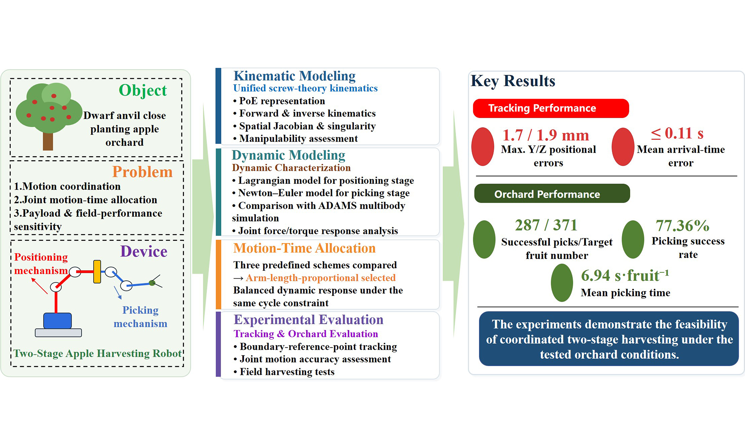
Abstract
A two-stage apple-harvesting robot was analyzed to improve motion coordination and harvesting efficiency in dwarf and high-density orchards. Screw theory was used to formulate the forward and inverse kinematics and spatial Jacobians of the positioning and picking mechanisms, while the Lagrangian and Newton–Euler methods were used to establish their dynamic models. Three predefined joint motion-time allocation schemes were compared under the same cycle constraint, and the link-length-proportional scheme was selected for subsequent analysis and experiments because it produced comparatively smooth actuator-load responses. Numerical comparison with an ADAMS rigid-body model showed close agreement under matched assumptions. Payload analysis indicated that the translational joint was most affected by increased fruit load. Planar boundary-point tracking tests produced maximum errors of 1.7 and 1.9 mm in the Y and Z directions, respectively, while the maximum joint errors were 1.7° for revolute joints and 1.6 mm for the prismatic joint. Orchard experiments achieved 287 successful picks among 371 targets, corresponding to a pooled success rate of 77.36% (95% Wilson CI: 72.83%-81.32%), with a mean picking time of 6.94 s per fruit. These results demonstrate the feasibility of the proposed modeling and motion-parameter allocation framework under the tested orchard conditions.
Keywords


 Download PDF
1. INTRODUCTION
Statistics from the National Bureau of Statistics of China indicate that the country ranks first globally in both apple production and consumption, with a cultivation area of over 1.9 million hectares. In 2024, total apple output reached 51.2851 million tons, representing more than half of global production and reflecting a year-on-year growth of 3.39%[1]. Despite this scale, apple harvesting remains largely manual, accounting for approximately 30%-50% of the total production workload. With the widespread adoption of dwarf and high-density planting systems, characterized by narrow row spacing, thin canopies, and high fruit density forming a “wall-like” structure[2], higher requirements are imposed on the motion performance and operational efficiency of harvesting equipment compared with traditional orchards. In recent years, extensive research has been conducted in three main areas: vibration harvesting, platform-based operations, and robotic technologies[3-7], with most studies focusing on functional implementation. As the core execution unit of harvesting equipment, the motion characteristics of the picking mechanism directly affect operational efficiency in complex and dense canopy environments, making systematic and in-depth investigation essential[8-10].
Agricultural robots must operate reliably in unstructured field environments with uneven terrain and external disturbances. Bio-inspired designs offer lightweight structures, flexible locomotion, and strong environmental adaptability, while dynamic modeling supports structural optimization and stable motion control. Recent advances in thrust-vectoring and coordinated multi-limb actuation provide valuable insights for developing agile, stable, and multimodal agricultural robots[11,12]. Although these platforms address different operating environments, they illustrate the broader importance of analyzing the interaction among mechanism configuration, actuation allocation, and dynamic performance. The motion characteristics of harvesting mechanisms encompass multiple aspects, including motion accuracy, joint kinematic parameters, and dynamic performance. Existing studies have addressed these aspects from perspectives such as structural optimization, trajectory planning, control strategies, and dynamic analysis. In terms of structural and performance optimization, parameter optimization and multi-objective design methods have been shown to improve positioning accuracy, structural compactness, and overall motion performance[13,14]. Regarding kinematic modeling and singularity analysis, evaluating the workspace and transmission performance based on kinematic models helps avoid singular configurations[15]. In terms of motion smoothness and control performance, the integration of dynamic modeling with trajectory optimization or control algorithms - such as iterative learning control and path curve optimization - can improve trajectory tracking accuracy and suppress vibration to a certain extent[16,17]. Furthermore, lightweight design and key component optimization based on dynamic models have been shown to reduce driving torque and overall system mass[18]. For trajectory planning in complex environments[19], some studies have combined rapidly exploring random trees (RRT) with particle swarm optimization (PSO)[20] to achieve time-optimal trajectory planning for robotic manipulators under obstacle avoidance constraints, improving both trajectory diversity and search efficiency. In the field of control, iterative learning control has been applied to parallel robots to enhance tracking accuracy under high-speed motion by utilizing historical error information[21].To address the limited motion accuracy and coordinated joint-performance constraints encountered during harvesting in dwarf and high-density apple orchards, this study investigates the motion characteristics of a previously developed two-stage apple-picking mechanism. Ref.[22] is the direct predecessor of the present work and reports the mechanical design, workspace analysis, inverse-kinematic implementation, control system, and preliminary field evaluation of the same domain-segmented harvesting platform. Accordingly, the present study retains the physical architecture, agronomic domain definition, principal link dimensions, and basic control system described in Ref.[22], and these components are not claimed as new contributions. Building on this
The contributions of this study are threefold. First, a unified product-of-exponentials (POE) representation is developed for the two structurally distinct serial mechanisms, enabling consistent forward-kinematic, inverse-kinematic, Jacobian, and singularity analyses. Second, analytical dynamic models are established separately for the positioning and picking stages and are quantitatively validated, providing a basis for examining payload- and motion-cycle-dependent variations in joint forces and torques. Third, a constrained engineering method for joint-motion time allocation is investigated by comparing three predefined allocation rules, after which the selected configuration is evaluated through physical tracking and orchard experiments. Thus, the proposed approach should be regarded as a reproducible procedure for motion-parameter allocation and engineering performance evaluation rather than as a general-purpose mathematical optimization algorithm. A component-by-component comparison between Ref.[22] and the present study is provided in Table 1.
Comparison of inherited components and new contributions between Ref.[22] and the present study
| Component | Ref.[22] | Present study |
| Robot structure and prototype | Developed and tested | Same platform retained |
| Agronomic domain definition | Reported | Retained |
| Link dimensions | Reported | Retained |
| Forward kinematics | D–H formulation | PoE/screw-theory formulation |
| Picking inverse kinematics | Random-point geometric method | Method retained and cited |
| Jacobian and singularity analysis | Not systematically reported | Added |
| Analytical dynamics | Not systematically derived | Lagrange and Newton–Euler models added |
| Joint-time allocation | Baseline controller | Quantitative comparison of three schemes |
| Payload/cycle analysis | Not reported | Added |
| Main contribution | Device design and feasibility | Kinematic–dynamic characterization and parameter allocation |
2. MECHANISM STRUCTURE AND OPERATING PRINCIPLES
2.1. Agronomic characteristics and workspace definition of the target orchard
Dwarf and high-density planting is a core cultivation mode for the intensive development of the modern apple industry[23], offering significant advantages such as high yield, superior fruit quality, and strong adaptability to mechanized operations. To quantitatively characterize the three-dimensional spatial distribution of apples in such orchards and to facilitate subsequent workspace analysis and mechanism parameter design, A tree-based coordinate system is defined by taking the intersection of the trunk and the ground as the origin [Figure 1]. In this coordinate system, the Xt-axis is aligned with the inter-row direction to describe the distribution of fruits across row spacing; the Yt-axis is aligned with the in-row (plant spacing) direction to represent the spatial position of fruits along the tree row; and the Zt-axis is defined as vertically upward from the ground to characterize the vertical distribution of fruits. For the orchard conditions considered in this study, mature tree height is approximately 2.8-3.1 m. In the orchard used for field harvesting experiments, the average inter-row spacing and intra-row tree spacing were approximately 3.0 and 2.0 m, respectively. Fruits are primarily distributed at heights of 700-2,600 mm above the ground and within a horizontal distance of 0-800 mm from the trunk. Accordingly, the picking workspace of a single tree can be approximated as a cuboid with dimensions of 1,600 mm × 300 mm × 1,900 mm.
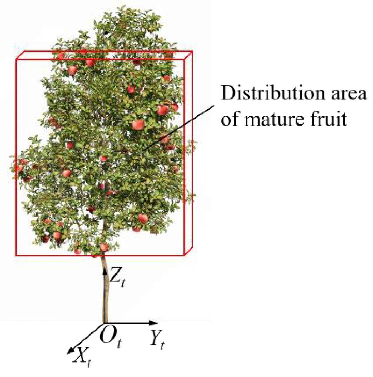
Figure 1. The distribution area of mature fruits on a single apple tree.
Figure 2 illustrates the overall configuration of the two-stage partitioned apple harvesting robot developed for dwarf and high-density orchards. The system includes a chassis, a support frame, a positioning module, and a picking module. The positioning module is composed of a support arm, a lifting arm, and a rotating main arm. The picking mechanism consists of a rotating secondary arm, a translational arm, a picking main arm, and a picking secondary arm.
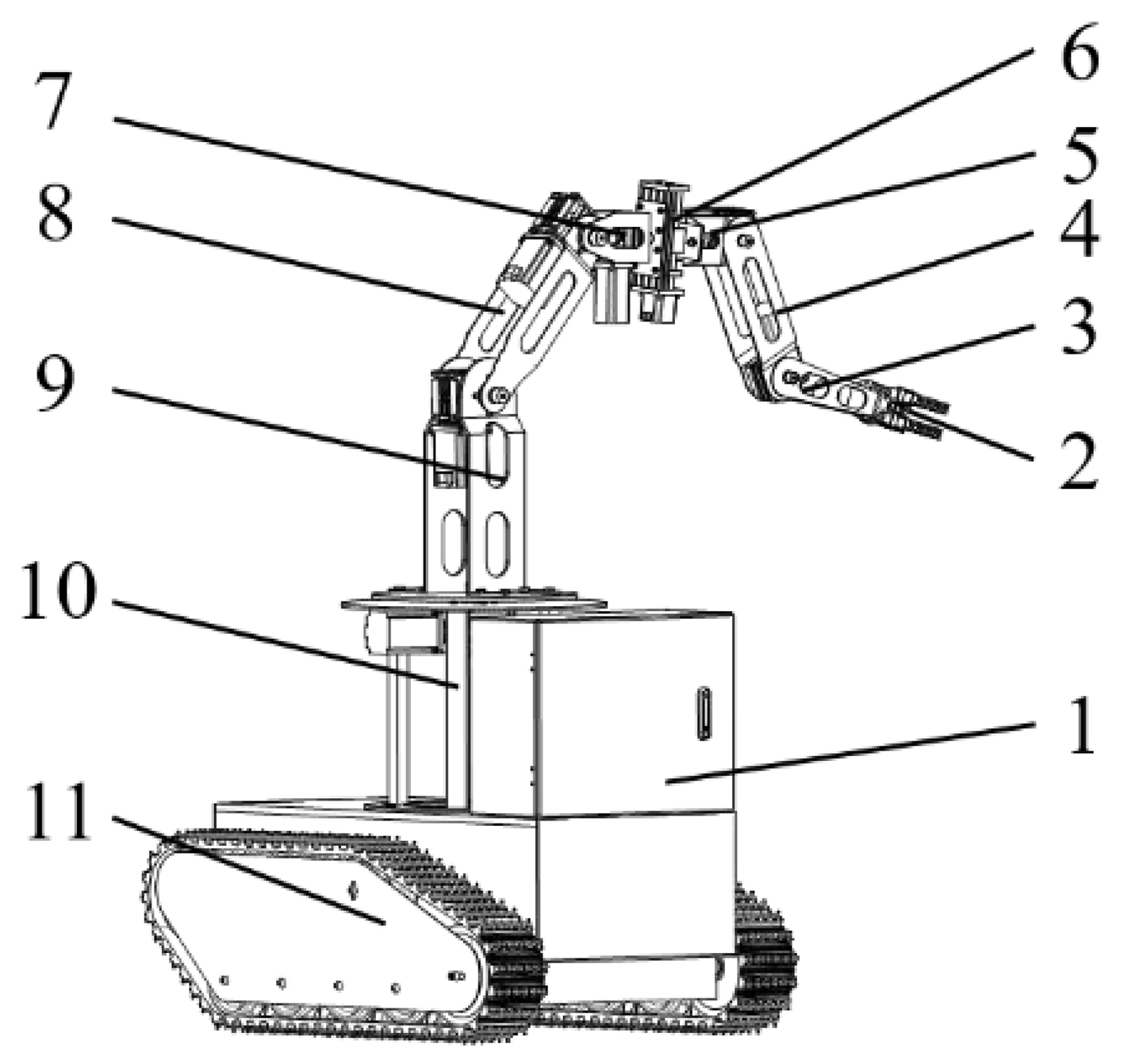
Figure 2. Overall structure of the apple harvesting robot. 1 denotes the control box; 2 denotes the end-effector (gripper); 3 denotes the picking secondary arm; 4 denotes the picking main arm; 5 denotes the translational arm; 6 denotes the rotating secondary arm; 7 denotes the rotating main arm; 8 denotes the lifting arm; 9 denotes the support arm; 10 denotes the frame; and 11 denotes the chassis.
2.2. Mechanism structure
The positioning mechanism adopts a 3R serial manipulator configuration, which is primarily used to achieve rapid positioning and posture adjustment of the picking base point within a single workspace. The picking mechanism employs an R–P–R–R joint configuration, enabling precise grasping and detachment of fruits within the picking region after base-point positioning is completed. The control system consists of a coordinated upper-level and lower-level architecture. The upper-level system, developed based on MATLAB and Python, is responsible for motion planning and task scheduling, while the lower-level system, centered on a microcontroller, performs motion control and execution feedback. This configuration enables the integration of autonomous harvesting and human–machine collaborative operations.
During operation, the center point at the end of the rotating main arm is defined as the positioning reference point of the device, whereas the grasping center of the end-effector is defined as the actual picking point. The main technical parameters of the robot are listed in Table 2.
Main technical parameters of the apple harvesting robot
| Parameters | Value |
| Applicable inter-row spacing for mobile-platform operation / m | 2.5-3.5 |
| Working height / m | 2.4 |
| Working width / m | 2.0-2.1 |
| Degree of freedom / units | 7 |
| Walking speed / m·s-1 | 0.9-1.1 |
The robot adopts a hierarchical motion-execution architecture. Target fruit coordinates are treated as task-level inputs to the motion system. The upper-level program, developed using MATLAB and Python, performs coordinate transformation, inverse-kinematic calculation, joint-command generation, and sequential task scheduling. The lower-level microcontroller executes the prescribed joint commands and returns motion-execution status to the upper level. The present study focuses on model-based motion generation and coordinated execution after a target coordinate has been provided. Fruit detection, multimodal sensor fusion, online obstacle avoidance, adaptive control, and autonomous target-selection strategies are outside the scope of the current work and are not evaluated experimentally. This scope distinction is important because the reported harvesting performance reflects the combined influence of the mechanical system and the prescribed motion-execution strategy rather than the performance of a complete autonomous perception-and-decision system.
2.3. Operating principles
Considering the spatial distribution of fruits and the canopy thickness in dwarf and high-density apple orchards, the picking workspace for a single tree can be simplified.To ensure full coverage of the fruiting area, the workspace is approximated as a cuboid measuring 1,600 mm × 300 mm × 1,900 mm. To reduce redundant motions and posture adjustments caused by cross-region operations of the manipulator, the cuboid workspace is symmetrically divided along the trunk direction into two independent target picking regions, denoted as U1 and U2, with the fruit partition plane serving as the symmetry reference, as shown in Figure 3A.
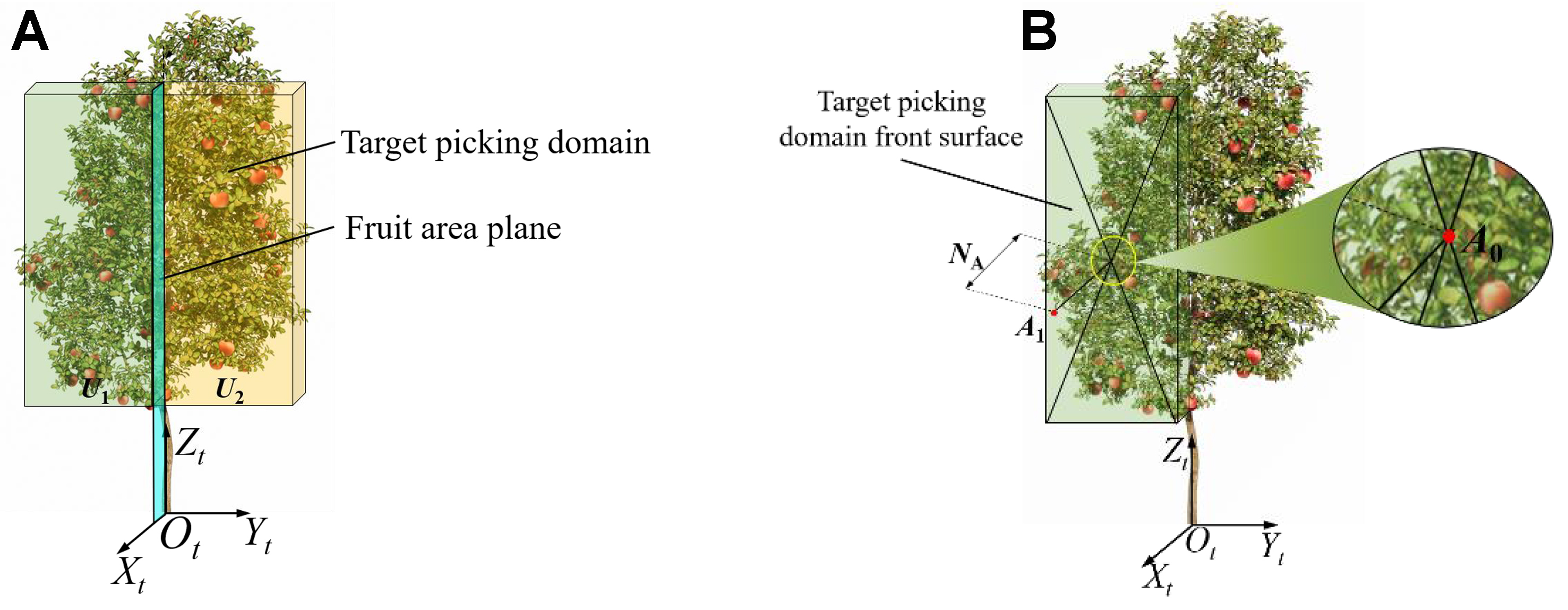
Figure 3. This figure illustrates the partitioning of the picking regions and the definition of the operational base point. (A) Schematic of fruit picking region partitioning; (B) Picking operation base point.
To minimize time loss caused by frequent repositioning and repeated adjustments during harvesting, and to improve the overall efficiency within a single picking region, a “single positioning–multiple picking” operation mode is adopted for each target region. Using the left picking region U1 as an example, the geometric center of its front surface is taken as point A0, representing the spatial center of the region. Taking into account the safety clearance between the end-effector and the fruit, along with structural installation constraints, point A0 is shifted 300 mm along the positive Xt-axis to obtain point A1. Point A1 serves as the positioning reference for single-region harvesting, and its coordinates are expressed as (XA, YA, ZA) [Figure 3B].
To accurately describe the spatial configuration of the harvesting robot, a base coordinate system (denoted as the X−Z−Y coordinate system) is established with the center of the support base as the origin. During operation, the chassis is positioned between two rows of trees, aligning the vertical column with one-quarter of the canopy width, as shown in Figure 4. During harvesting, the target joint angles of the lifting arm and the rotating main arm are determined via inverse kinematics based on the coordinates of the picking base point. The control system commands the motors to move the positioning reference point - corresponding to the end of the rotating main arm - to the specified base location. Target fruit coordinates expressed in the XtYtZt frame are then converted into the base coordinate system using MATLAB. Joint variables are subsequently obtained from the inverse kinematics of the picking mechanism and sent to the microcontroller through a Python interface, enabling the mechanism to complete automated harvesting.
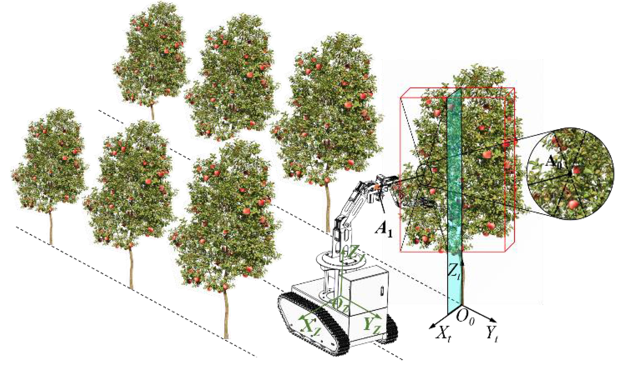
Figure 4. Schematic of the operating principle of the apple harvesting robot.
3. KINEMATIC MODELING AND ANALYSIS
3.1. Forward kinematic modeling
Compared with the conventional Denavit-Hartenberg formulation, the POE representation describes each joint directly through its screw axis in a common reference frame, without requiring the successive construction of link-attached coordinate frames or the selection of different DH conventions. This feature is particularly suitable for the present robot because it consists of two structurally different serial subsystems, namely a 3R positioning mechanism and an R-P-R-R picking mechanism. The screw-axis representation allows both mechanisms to be modeled within a consistent mathematical framework and enables the corresponding spatial Jacobians and singularity conditions to be derived directly from the same set of screw parameters. Therefore, the advantage considered in this study is primarily modeling consistency, geometric interpretability, and convenient singularity analysis, rather than experimentally demonstrated computational-speed improvement.
Based on the established geometric configuration and dimensions of the robot[22] (with key parameters listed in Table 3), the positioning and picking mechanisms are modeled separately. Their forward kinematics are established based on the segmented structural design.
Technical specifications of the harvesting system
| Mechanism | Component | Arm length / mm |
| Positioning mechanism | Frame d0 | 370 |
| Support arm l1 | 370 | |
| Lifting arm l2 | 650 | |
| Rotating main arm l3 | 200 | |
| Picking mechanism | Rotating secondary arm l4 | 100 |
| Translational arm l5 | 200 | |
| Picking main arm l6 | 600 | |
| Picking secondary arm l7 | 400 |
The instantaneous motion of a rigid body is characterized by its linear and angular velocity components. For a clearer representation within screw theory, the twist ξ is normalized and formulated using the PoE[24] approach. Accordingly, the rotational motion of the rigid body can be expressed as:
Note: All arguments of the matrix exponential and the trigonometric functions in Equations (1)-(14) are dimensionless, and all revolute-joint variables are therefore evaluated in radians. where Si denotes the normalized motion twist in the initial configuration; I is the 3 × 3 identity matrix; θi represents the joint variable; ωi is the angular velocity about the screw axis of the i-th joint; vi is the linear velocity along the screw axis of the i-th joint; [ωi] is defined as the 3 × 3 skew-symmetric matrix derived from the angular velocity ω,
Angular velocity and angular acceleration are expressed in rad·s-1 and rad·s-2, respectively. For a prismatic joint, θi denotes translational displacement; millimeters are used for engineering reporting, while meters are used in SI-based dynamic calculations.
At the initial configuration, the PoE-based forward kinematic description is fully determined by specifying the base frame {s} and the end-effector frame {b}. Under this condition, the forward kinematics takes the following POE form:
Here, T corresponds to the end-effector pose relative to the base frame, while M specifies its initial configuration. The symbol n indicates the total number of joints in the mechanism, and this notation is used consistently throughout the remainder of the paper.
Let the initial pose matrices of the positioning mechanism and the picking mechanism be denoted as M1 and M2, respectively, where the reference point for each is defined as the origin of its end-effector frame. Their corresponding coordinates are given by:
Figure 5 presents the coordinate frames at the initial configuration of each mechanism, while the associated screw axis parameters S are provided in Tables 4 and 5.
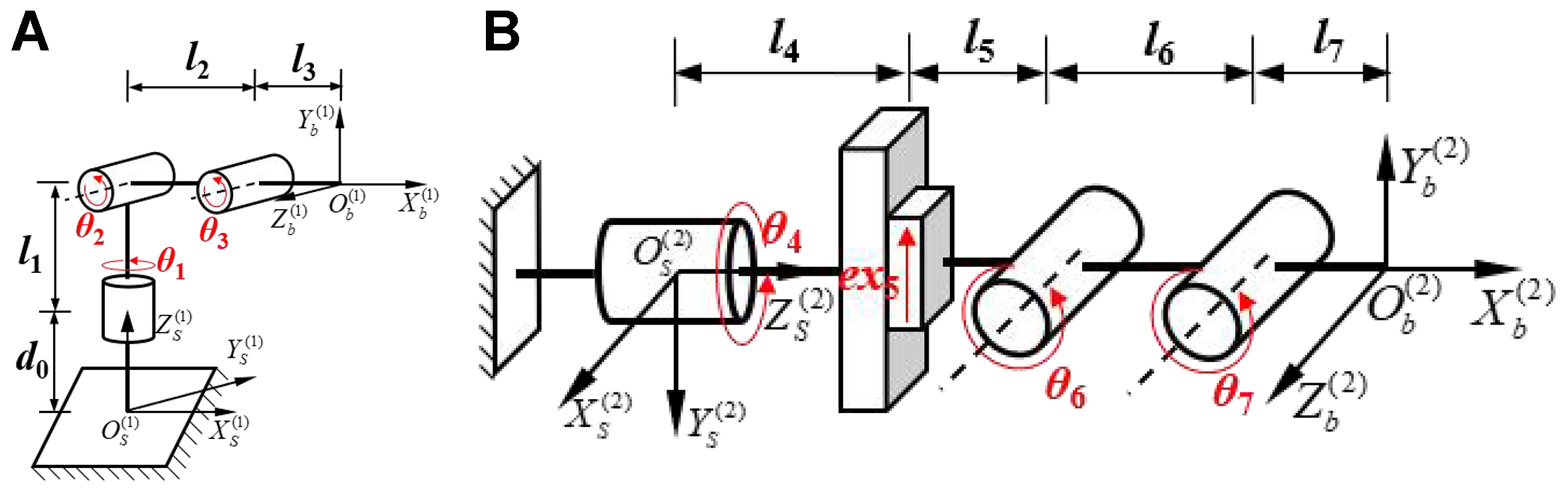
Figure 5. Screw coordinate systems of the harvesting robot. (A) Initial configuration of the positioning mechanism; (B) Initial configuration of the picking mechanism. OS(1) - XS(1)YS(1)ZS(1) and OS(2) - XS(2)YS(2)ZS(2) denote the base coordinate frames of the positioning mechanism and the picking mechanism, respectively; Ob(1) - Xb(1)Yb(1)Zb(1) and Ob(2) - Xb(2)Yb(2)Zb(2) denote the coordinate frames of the positioning base point and the end-effector (gripper) reference point, respectively.
Screw axis parameters of the positioning mechanism
| i | q | ωi | vi |
| 1 | (0, 0, d0) | (0, 0, 1) | (0, 0, 0) |
| 2 | (0, 0, d0+l1) | (0, -1, 0) | (d0+l1, 0, 0) |
| 3 | (l2, 0, d0+l1) | (0, -1, 0) | (d0+l1, 0, -l2) |
Screw axis parameters of the fruit-picking mechanism
| i | q | ωi | vi |
| 4 | (0, 0, 0) | (0, 0, 1) | (0, 0, 0) |
| 5 | (0, 0, l4+l5) | (0, 0, 0) | (0, -1, 0) |
| 6 | (0, 0, l4+l5+l6) | (1, 0, 0) | (0, l4+l5, 0) |
| 7 | (0, 0, l4+l5+l6+l7) | (1, 0, 0) | (0, l4+l5+l6, 0) |
Using Equation (2) together with the parameters in Tables 4 and 5, the forward kinematics of the positioning and picking mechanisms are derived as follows:
where σ1 = l2(c3 - 1) - s3(d0 + l1); σ2 = l2s3 + (d0 + l1)(c3 - 1); s23 = sin(θ2 + θ3); c23 = cos(θ2 + θ3), and the same notation applies hereafter.
where θ5 denotes the displacement of the prismatic joint (mm), s67 = sin(θ6 + θ7), c67 = cos(θ6 + θ7), and the same notation applies hereafter.
The accuracy of the screw-theory-based forward kinematic models is examined by simplifying the fourth columns of Equations (3) and (4) and comparing them with the corresponding entries in the pose matrices reported in Ref.[22]. Full agreement is observed, which validates the correctness of the models.
3.2. Inverse kinematics
According to the structural characteristics of the robot, the inverse kinematics are solved using the variable separation method[25] and the geometric–random point method (see Ref.[22] for details), respectively. Based on the variable separation approach, let the spatial position of the positioning reference point [i.e., the origin of the (X3Y3Z3) coordinate frame] in the (X0Y0Z0) coordinate frame be (x, y, z). According to Equation (2), the corresponding transformation matrices can be derived as follows:
To ensure dimensional consistency in the matrix operations, the position of the positioning base point is reformulated in homogeneous coordinates as (x, y, z, 1)T. Accordingly, the elements of the known end-effector pose matrix are equated with the corresponding elements of the positioning base point vector.
where
Let r = x2 + y2 + z2 be defined accordingly and substitute it into Equation (5), yielding r = l32 + l22 + 2l2l3cosθ3. Therefore, the joint angle θ3 can be expressed as:
From Equation (6), let R1 =
From Equation (7), let R2 =
3.3. Jacobian matrix and singularity analysis
Kinematic singularities cause a robot’s end-effector to lose mobility in certain translational or rotational directions. To quantitatively evaluate this phenomenon and enable visualization, the Jacobian matrix[26] is used to establish the mapping between joint velocities and end-effector velocity. A manipulability index then characterizes the robot’s proximity to singular configurations at a given pose. The spatial velocity Vs can be expressed as:
Here, Js(θ) represents the space Jacobian defined in the fixed (space) frame, while
The i-th column Jsi(θ) of the Jacobian corresponds to the twist associated with the i-th joint axis in the fixed (space) frame. Its expression is given by
where the first column Js1 = S1; Ti-1 =
In this formulation, the twist coordinates of the i-th joint after the rigid-body transformation Ti-1 are denoted by
Based on Equations (8) and (9), the Jacobian matrices of the positioning mechanism (denoted as Jc) and the picking mechanism (denoted as Jz) can be expressed as follows:
To evaluate the motion performance of the mechanism and avoid the occurrence of singular configurations, singularity analysis is conducted based on the rank properties of the Jacobian matrix and the manipulability index. The Jacobian matrix of the positioning mechanism, Jc, is a 6 × 3 matrix. When the second and third column vectors become linearly dependent, the joint angle θ2 takes a value of 90°. In addition, the fourth and fifth elements of the corresponding column vectors must be equal, satisfying the following condition:
The solution shows that no valid value exists for θ1, indicating that the second and third column vectors are linearly independent. Furthermore, the third column vector cannot be expressed as a linear combination of the other two columns; therefore, the rank of Jc is 3 (full rank), and the positioning mechanism does not exhibit kinematic singularities.
Similarly, for the Jacobian matrix Jz, if the third and fourth column vectors are linearly dependent, the following condition must be satisfied:
Solving the above condition yields θ6 = π/2 and θ4 = 0.81π. Further examination of the third row elements indicates that the first three column vectors are linearly independent. Therefore, the rank of Jz is 3 (less than its column number of 4), implying that the mechanism is rank-deficient and a kinematic singularity exists at this configuration.
Manipulability is an important metric for quantifying the motion capability of a robot end-effector in task space. Based on this index, the motion capabilities of the picking mechanism along the X-, Y-, and Z-axes are quantitatively evaluated. The manipulability ratio μ1 is adopted as the evaluation parameter, which characterizes the relative ease of motion in different directions at a given pose (μ1 ≥ 1). The specific formulation is given as:
Here, A is a 6 × 6 matrix, and J represents the Jacobian. The quantities λmax and λmin correspond to the largest and smallest eigenvalues of JJT, respectively.
Based on Equation (14), the analysis is conducted in conjunction with the picking mechanism’s initial configuration. The initial configuration parameters are summarized in Table 6.
Initial setup parameters of the picking mechanism
| Name | Rotating secondary arm / ° | Translational arm / m | Picking main arm / ° | Picking secondary arm / ° |
| Initial configuration values | 0 | 0 | 0 | 0 |
The geometric characteristics of the manipulability ellipsoid indicate that when μ1 approaches 1, the ellipsoid tends toward a spherical shape, exhibiting strong isotropy, and the mechanism’s manipulability becomes nearly uniform in all directions. As μ1 increases, the ellipsoid becomes increasingly elongated, indicating that motion along its principal axis is significantly better than in other directions. When μ1 approaches infinity, the mechanism tends toward a kinematic singular configuration.
Based on Equation (11) and Table 6, the Jacobian matrix of the picking mechanism at the initial configuration (with arm length parameters expressed in SI units, i.e., meters) yields eigenvalues of (0, 0, 0, 1, 3.15) and (0.75). Substituting these into Equation (11) shows that μ1 approaches infinity at the initial configuration, indicating the presence of a kinematic singularity.
4. DYNAMIC MODELING AND VALIDATION
4.1. Dynamic modeling of the positioning mechanism
To further investigate the motion characteristics of the positioning mechanism, a dynamic analysis is conducted[27,28]. Considering its operating requirements and structural features, a dynamic model is established using the Lagrangian formulation[29]. The independent generalized coordinates are chosen as q1 and q2, corresponding to the rotation angles of the lifting arm and the rotating main arm, respectively. The Lagrangian function L(q,
where K is the total kinetic energy of the mechanism, and P is the total potential energy.
Based on the fundamental form of the Lagrangian function, the dynamic equations can be expressed as:
where τ denotes the non-conservative generalized force acting on the mechanism.
Due to its limited rotational range and negligible impact on overall system dynamics, the support arm is not considered in the analysis; the dynamic modeling focuses on the lifting arm and rotating main arm (hereinafter referred to as the “key links”). The support arm remains stationary during the harvesting operation and serves only as a structural base for the positioning mechanism. It is retained in the geometric description to define the installation height and base coordinate frame, but it is not assigned an independent generalized coordinate and does not contribute a kinetic-energy term to the dynamic equations. Therefore, the dynamic analysis focuses on the lifting arm and the rotating main arm.
The corresponding model is shown in Figure 6. The positioning mechanism is represented by three physical links: the support arm, lifting arm, and rotating main arm, with masses m1, m2, and m3, respectively. The two moving links are the lifting arm and rotating main arm, whose generalized coordinates are q1 and q2, respectively. The center-of-mass distances of the three physical links are denoted by lc1, lc2, and lc3.
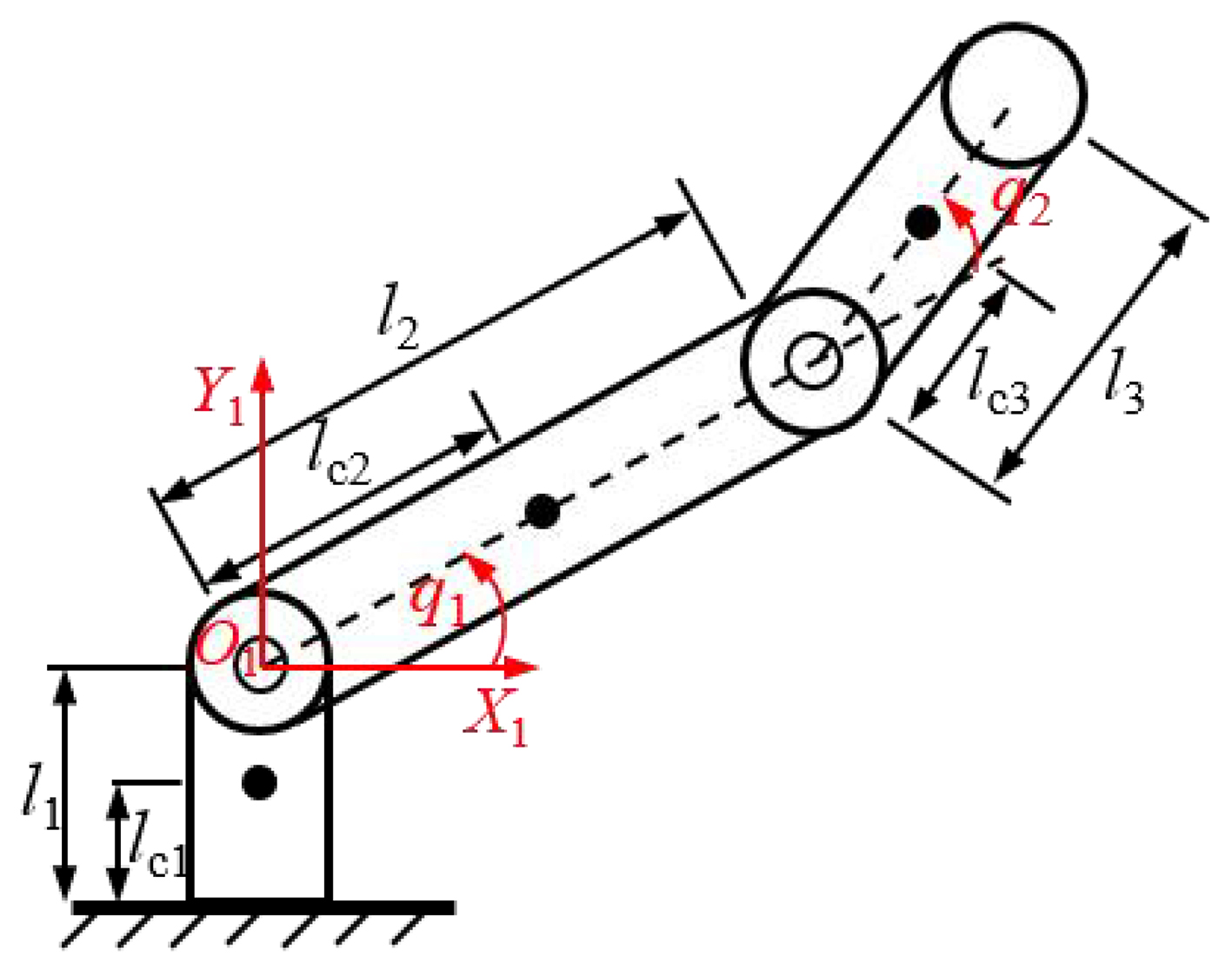
Figure 6. Coordinate systems and link length parameters of the dynamic model. l1, l2, and l3 are the lengths of the Support arm, lifting arm, and Rotating main arm, respectively.
The bottom surface of the support arm is selected as the zero-potential-energy reference plane. With this choice of reference plane, the gravitational potential energy of m1 must be included. Therefore, the total potential energy of the system is expressed as:
With the X1O1Y1 frame [Figure 6] defined as the reference frame, the rotation matrix and position vector of the centroid of the i-th link relative to this frame are obtained as follows, where the rotation matrix is denoted as Ri and the centroid displacement vector is denoted as Oci0, respectively:
Using Equation (9), the centroid Jacobian Jci is formulated to relate joint velocities to the centroid velocities of each link. On this basis, the total kinetic energy of the system is given by:
In this formulation, M refers to the 2 × 2 inertia matrix, while
Each link is treated as a rigid body, and joint friction is neglected. Under these conditions, the dynamic equation of the mechanism is given by
Here, M denotes a symmetric positive-definite matrix reflecting the effect of joint accelerations on the system dynamics. Based on Equation (18), it can be obtained that:
From Equation (19), it can be seen that C(q,
where cijk denotes the Christoffel symbols of the first kind. Based on the above equation, it can be obtained that C =
Based on Equations (19) and (20), it can be obtained that G =
The dynamic model of the positioning mechanism establishes the mapping relationship between the driving torques and the motion states based on the matrices M, C, and G, providing a fundamental theoretical basis for dynamic performance analysis and parameter identification.
4.2. Dynamic modeling of the picking mechanism
The picking mechanism exhibits a multi-degree-of-freedom serial configuration, and its dynamics are modeled using the Newton–Euler recursive approach[30]. Geometric parameters of the links are summarized in Table 3, while their corresponding masses are provided in Table 7. A schematic representation of the dynamic model is presented in Figure 7.
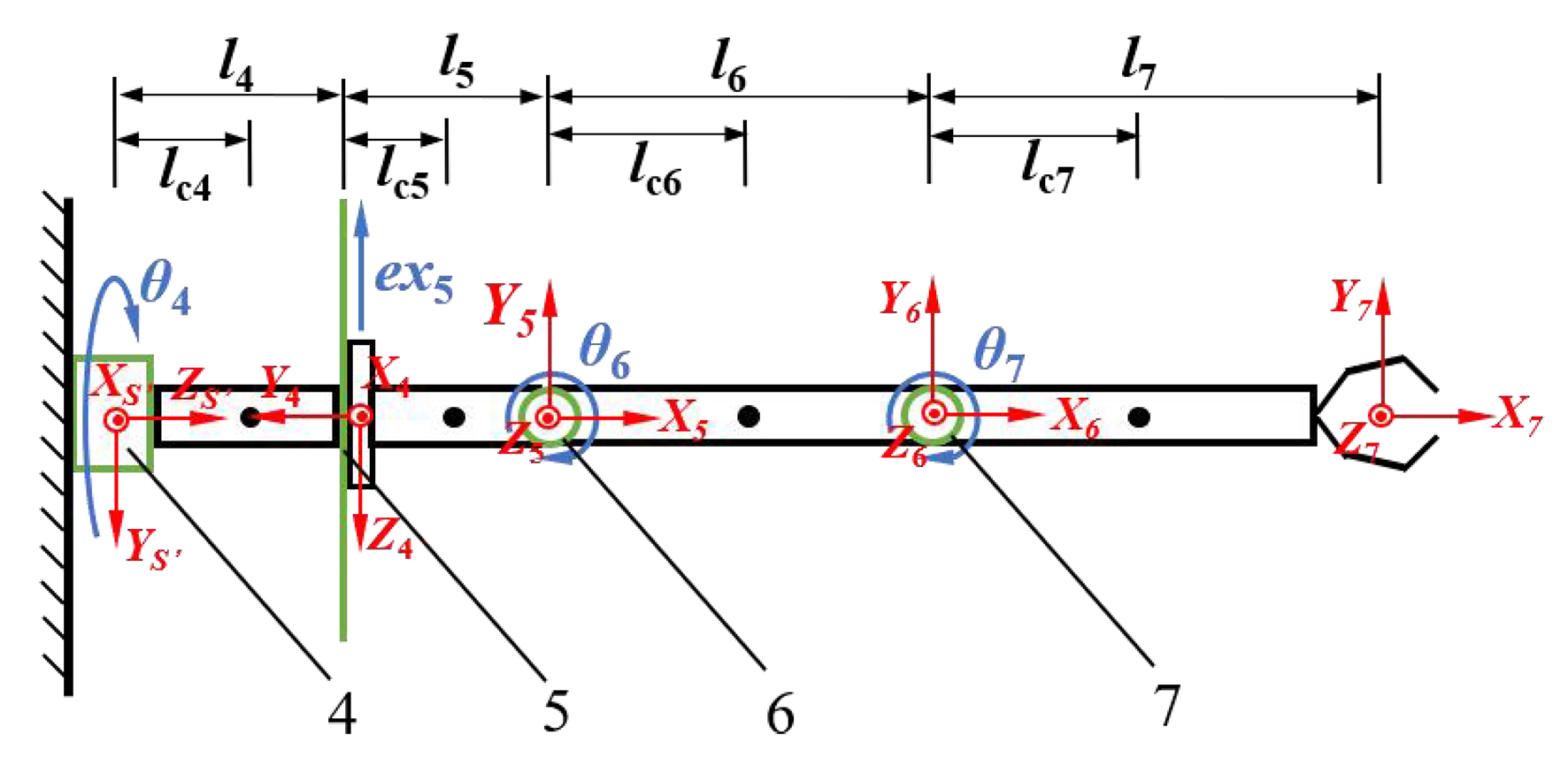
Figure 7. Dynamic model of the picking mechanism. O0’X0’Y0’Z0’ denotes the initial coordinate frame of the picking mechanism; joints 4-7 correspond to joints 4-7, respectively. The axes Xi, Yi, and Zi (i = 4, 5, 6, 7) correspond to the coordinate frame OiXiYiZi attached to joint i. Among these joints, 4, 6, and 7 are rotational, whereas joint 5 is translational. The positive directions of the XS′, X4, Z5, and Z6 axes are perpendicular to the plane of the page and point outward.
Mass parameters of each link in the picking mechanism
| Name | Rotating secondary arm | Translational arm | Picking main arm | Picking secondary arm |
| Mass / kg | 1.155 | 1.009 | 2.188 | 1.73 |
Each link is assumed to be a symmetric rigid homogeneous body, with its mass concentrated at the geometric center. The distances between each center of mass and its corresponding joint are defined as lc4, lc5, lc6, and lc7.
The Newton–Euler dynamic formulation, derived from rigid-body kinematics and dynamics, is carried out in two stages: first, a forward recursion is performed to compute the velocities and accelerations of each link; then, a backward recursion is carried out to determine the joint driving forces (torques). The transformation matrix T enables the propagation of kinematic variables between adjacent links. The pose transformation between neighboring joints can be obtained from Equation (2).
Considering the actual picking operation state and the structural characteristics of the robot, the initial conditions and joint motion types are defined. When the end-effector grasps an apple, it is subjected to the gravitational vector g acting vertically downward. At the initial operation stage, the mechanism is in a static state, and the initial kinematic parameters are given as follows: All θ1,
The forward recursion starts from the rotating secondary arm and proceeds sequentially along each link to the end-effector (picking point), yielding the angular velocity, angular acceleration, linear velocity, and linear acceleration of each link. The corresponding kinematic equations are given as follows:
Here, i represents the joint index (i = 3, 4, 5, 6, 7). The unit vector along the Z-axis of joint i+1 is given by i+1
Based on Equations (21)-(24), the kinematic equations of the centroid acceleration are given as follows:
The centroid linear acceleration of link i+1, expressed in the i+1-th joint frame, is given by i+1
Based on Equation (25), the force and moment equations at the link centroid are given as follows:
The mass of link i+1 is given by mi+1 (kg), and its centroidal inertia is described by the matrix
Based on Equations (26) and (27), the forces and moments acting on each link are first computed. Then, the corresponding joint driving forces and torques under the given loading conditions are obtained using the backward recursion formulation.
The driving force acting on link i, expressed in the i-th joint coordinate frame, is represented by ifi (N), with analogous definitions applied to subsequent terms. The corresponding driving torque in the same frame is denoted by i+1fi+1 (N·m).
Using Equations (28) and (29), the joint forces and torques are derived by projecting the forces (and moments) between adjacent links onto the Z-axis, as expressed below:
Here, qfi represents the driving force of the i-th joint, while qτi corresponds to the driving torque of the same joint.
From the above dynamic equations, the dynamic model of the picking mechanism is obtained. Given that the harvesting task primarily depends on the main functional components, this work derives the joint torque expressions for the picking main arm and secondary arm. For brevity, the dynamic equations of the remaining joints are not presented.
where τ6 denotes the joint torque of the picking main arm;
σ1 = 118.0451c6s7 + 92.563438s67c67 + 0.6651c6σ8 + 203.4798c7s67c67
+ 1.02s7s67s67 + 1.02σ4 + 1500c7 - 0.3462s7σ5 + 0.3462c7σ4 + 880.88s7 + 1000;
σ2 = 1652.5119c6 + 16739.2266s4 + 830.8915c67 + c7σ6 + s7σ7 + 3.4127;
σ3 = 166.8981s6 - s7σ6 + c7σ7;
σ4 = 600c6s6 + c6σ8;
σ5 = 600s6s6 + s6σ8 + 600;
σ6 = 415.4458c6 + 3396.2691s4 + 337.6656c67 + 0.6924;
σ7 = 7.1967s67;
σ8 = θ5 + 9810c4.
where τ7 denotes the joint torque of the picking secondary arm;
σ1 = 415.4458c7 + 3396.2691s4 + 377.6656c67 + 0.6924;
σ2 = 92.564338s67c67 + 207.72s6c67 + 0.3462c67σ6 - 207.72s7;
σ3 = θ5 + 9810c4.
4.3. Numerical cross-verification of the ideal rigid-body dynamic model
To evaluate the numerical consistency of the analytical Newton–Euler implementation, a corresponding rigid-body multibody model was established in ADAMS. The analytical and ADAMS models use the same link geometry, mass properties, gravitational acceleration, prescribed joint trajectories, ideal-joint definitions, and external payload. Therefore, the comparison presented in this section is intended as numerical cross-verification between two independently implemented formulations under matched assumptions, rather than as independent physical validation of the prototype.
Simulation studies of joint dynamic parameters are conducted under representative operating conditions to assess the validity of the dynamic equations of the picking mechanism. A simplified three-dimensional model is first established in SolidWorks and then imported into ADAMS. Material properties and spatial pose parameters are assigned, and appropriate kinematic joints are defined according to the joint types to construct a multibody dynamic model, as shown in Figure 8.
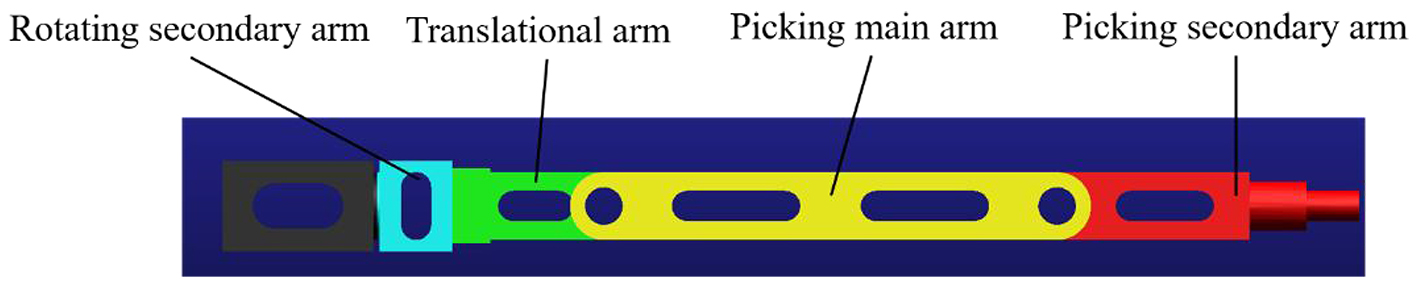
Figure 8. ADAMS-based simulation model of the picking mechanism.
Based on the simplified model, key simulation parameters are specified. The gravitational acceleration is set to g = 9.81 m/s2, while the link lengths and masses are given in Tables 3 and 7, respectively. Considering the actual harvesting conditions, this section focuses on the key links directly involved in fruit grasping and picking, namely the translational arm, the picking main arm, and the picking secondary arm, and analyzes their dynamic characteristics. For engineering readability, the commanded revolute-joint velocity is reported as 30°·s-1, corresponding to 0.5236 rad·s-1 in the analytical calculation. The prismatic-joint velocity is
To quantitatively evaluate model accuracy and eliminate the influence of magnitude differences, 240 sampling points are selected at intervals of 0.1 s. The relative error ηi at each time instant, as well as the mean relative error ηa, between the simulation data and the theoretical results are then calculated.
Here, DMi represents the value obtained from the MATLAB-based dynamic equations at the i-th sampling instant, while DAi corresponds to the simulation results generated by ADAMS at the same time step. The same notation is used consistently in the following sections. ηi corresponds to the relative error at the i-th sampling instant, and n indicates the total number of sampling points. This notation is maintained throughout the remainder of the paper.
Based on the simulation data and Equations (34) and (35), the mean relative error is calculated, and comparative plots of the theoretical and simulated joint forces and torques of the picking mechanism are generated [Figure 9].
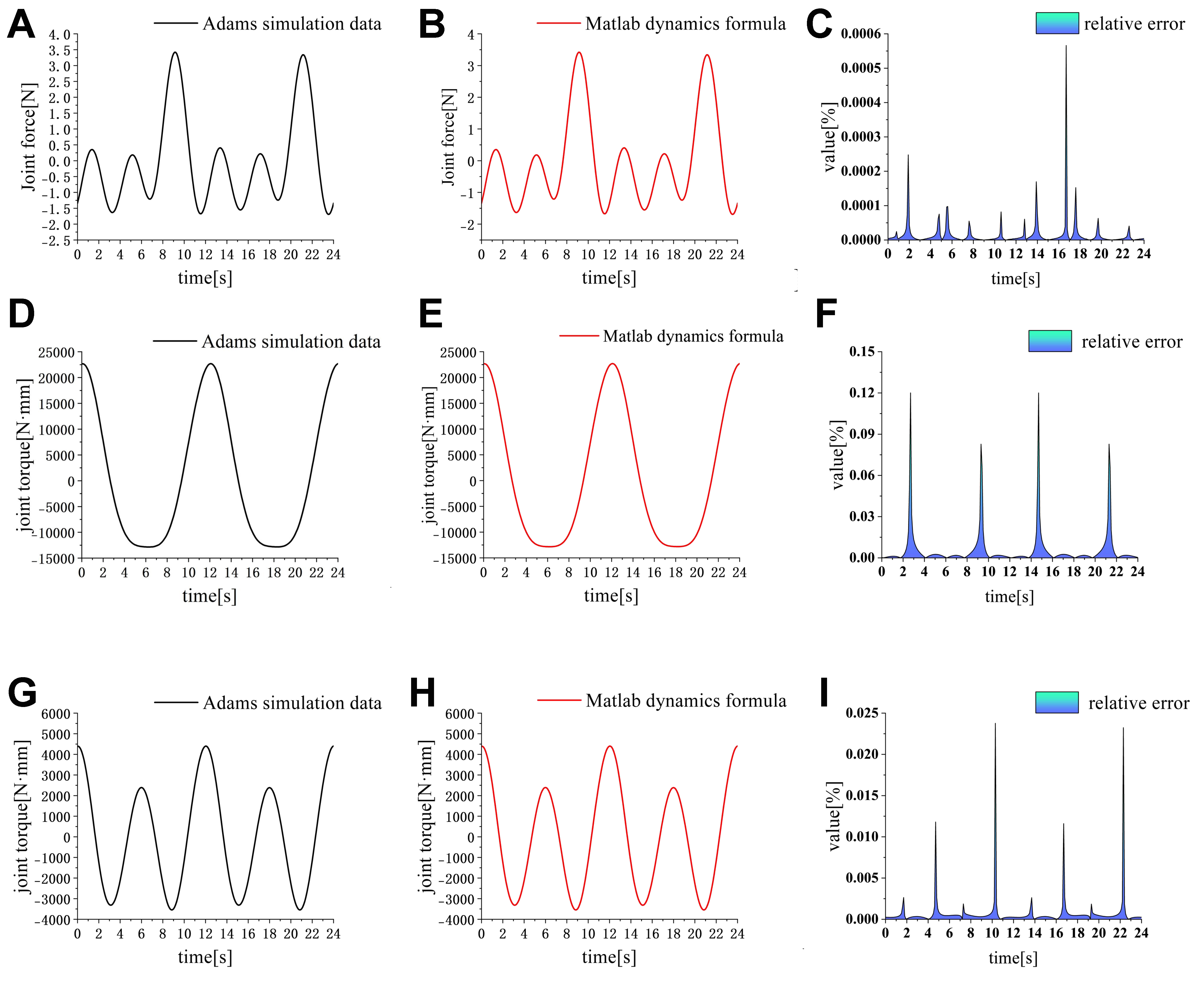
Figure 9. Comparison of joint forces and torques of the picking mechanism between MATLAB-based dynamic formulations and ADAMS simulation data. (A) ADAMS simulation of translational arm joint force; (B) MATLAB-based dynamic result of translational arm joint force; (C) Relative error of translational arm joint force; (D) ADAMS simulation of picking main arm joint torque; (E) MATLAB-based dynamic result of picking main arm joint torque; (F) Relative error of picking main arm joint torque; (G) ADAMS simulation of picking secondary arm joint torque; (H) MATLAB-based dynamic result of picking secondary arm joint torque; (I) Relative error of picking secondary arm joint torque.
As shown in Figure 9C, F, and I, the mean relative errors of each link are 0.00152%, 0.598%, and 0.0856%, respectively. These errors mainly arise from the calculation of centroid inertia and the rounding errors introduced by truncation to three decimal places in the error analysis. The largest error occurs at the joint of the picking main arm, but it remains below 0.6%, which satisfies the accuracy requirements. This confirms the validity of the MATLAB-based dynamic formulations.
To quantitatively evaluate the linear correlation between the two dynamic curves corresponding to the same joint, the linear correlation coefficient r is adopted as the evaluation metric.
where
Based on Equation (36), the linear correlation coefficients of the joint curves are calculated as 0.999375, 0.999998, and 0.999999, respectively. These results indicate that all r values are close to 1, demonstrating a strong linear correlation between the corresponding curves.
To verify the accuracy of the model, we introduce the following calculation indicators.
Let the residual at the iii-th sampling instant be defined as
where DMi and DAi denote the analytical and ADAMS results, respectively. The following metrics are used:
Pearson’s correlation coefficient is calculated from the unrounded data. The phase lag is determined from the time shift corresponding to the maximum cross-correlation between the two curves. The calculation data are shown in Table 8 below.
MAE, RMSE, and MaxAE of force/torque predictions for the translational arm, picking main arm, and picking secondary arm
| Joint response | MAE | RMSE | MaxAE |
| Translational arm force | 0.000152 | 0.000470 | 0.000566 |
| Picking main arm torque | 0.005983 | 0.016577 | 0.12009 |
| Picking secondary arm torque | 0.000761 | 0.002479 | 0.02377 |
The force/torque errors of the translational arm, picking main arm, and picking secondary arm were evaluated using the mean absolute error (MAE), root mean square error (RMSE), and maximum absolute error (MaxAE). The results show that the translational arm has the lowest values for all three error metrics, indicating a high degree of agreement between the analytical and simulation results. The error level of the picking secondary arm lies between those of the translational arm and the picking main arm, and its overall agreement is better than that of the picking main arm. In comparison, the picking main arm exhibits the highest MAE, RMSE, and MaxAE among the three mechanisms, together with relatively pronounced instantaneous error peaks during motion, indicating comparatively large local deviations in its dynamic response.
Considering the three error metrics collectively, the errors of the translational arm, picking main arm, and picking secondary arm are all below the allowable error thresholds specified for the system. This result demonstrates good overall agreement between the dynamic-model predictions and the simulation results. Therefore, the accuracy and reliability of the established dynamic models are validated under the prescribed motion trajectory and operating conditions examined in this study.
The present model does not explicitly account for joint friction, reducer and transmission efficiency, mechanical backlash, structural compliance, motor and reducer inertia, closed-loop controller dynamics, or fruit–branch contact. These factors may cause differences between the predicted rigid-body actuator loads and the actual prototype responses. Calibrated joint-load or motor-current measurements are therefore required before the model can be considered physically validated.
5. JOINT MOTION-PARAMETER ALLOCATION AND SIMULATION ANALYSIS
5.1. Comparison of joint motion-time allocation schemes
The picking mechanism serves as the primary execution unit of the harvesting system, and precise control of its joint motions is essential for reliable operation. To compare candidate joint-velocity parameter configurations, numerical simulations were performed based on the established dynamic model and the prescribed boundary positions of the picking trajectory. The one-way reaching duration, defined as the prescribed time for the picking mechanism to move from its initial configuration to a boundary reference point, was fixed at Tr =7 s as an engineering constraint for the joint-time allocation analysis. This prescribed reaching duration should be distinguished from both the out-and-return simulation cycle used in Sections 5.2-5.3 and the experimentally measured single-fruit picking time reported in the orchard test. This value was selected with reference to the picking cycle time reported in Ref.[22], while also considering the motion range and actuator capability of the proposed mechanism. Throughout this manuscript, the terms “one-way reaching duration”, “out-and-return simulation cycle”, and “field single-fruit picking time” refer to different quantities and are used accordingly.
The joint-motion timing directly affects actuator loads and motion smoothness. Rather than performing continuous numerical optimization, we compare three predefined engineering allocation rules under the same fixed one-way reaching-duration constraint. These rules are equal-time allocation, link-length-proportional allocation, and mass-length-combined allocation. For each scheme, the motion time assigned to joint i is denoted by ti, satisfying
and the corresponding commanded joint velocity is calculated from
where Δqi is the prescribed motion range of joint i. The three schemes are evaluated under identical motion ranges, payload, and simulation conditions by comparing the amplitude, abruptness, and duration of the resulting joint-force and joint-torque fluctuations. Accordingly, the procedure is an engineering comparison of parameter-allocation rules rather than a mathematical optimization involving an iterative search algorithm. Table 9 summarizes the motion ranges of each joint at the boundary picking point of the mechanism.
Joint motion ranges at boundary picking points
| Parameter | Rotating secondary arm / ° | Translational arm / mm | Picking main arm / ° | Picking secondary arm / ° |
| Joint motion range | 45 | 100 | 60 | 30 |
Based on the one-way reaching duration and the parameters listed in Table 9, three predefined allocation strategies - namely, equal-time allocation, link-length proportional allocation, and mass–length combined allocation - are adopted to determine the joint velocity parameters, and simulations are conducted to compare the resulting joint-motion parameter configurations.
In the equal-time allocation strategy, the prescribed 7 s one-way reaching duration is equally allocated among the four joint motions. The parameters for the link-length proportional scheme and the mass–length combined scheme are defined as follows:
where li denotes the link length of the i-th arm of the picking mechanism (i = 4, 5, 6, 7); dLi is the allocation ratio based on the link-length proportion; and dMi is the optimization parameter based on the mass–length combined criterion.
According to the above allocation strategies, the joint-motion time allocation within the prescribed 7 s one-way reaching phase is obtained. The corresponding results are summarized in Table 10.
Motion parameters of key links under different allocation strategies
| Allocation strategy | Allocation parameter ratio | Motion time | Motion velocity | |
| Equal-time allocation strategy | Rotating secondary arm | 25% | 1.75 s | 25.71 °/s |
| Translational arm | 25% | 1.75 s | 57.14 mm/s | |
| Picking main arm | 25% | 1.75 s | 34.29 °/s | |
| Picking secondary arm | 25% | 1.75 s | 17.14 °/s | |
| Link-length-proportional allocation strategy | Rotating secondary arm | 7.69% | 0.54 s | 83.33 °/s |
| Translational arm | 15.38% | 1.08 s | 92.59 mm/s | |
| Picking main arm | 46.15% | 3.23 s | 18.58 °/s | |
| Picking secondary arm | 30.77% | 2.15 s | 13.95 °/s | |
| Mass–length-proportional allocation strategy | Rotating secondary arm | 4.97% | 0.35 s | 128.57 °/s |
| Translational arm | 8.69% | 0.61 s | 163.93 mm/s | |
| Picking main arm | 56.54% | 3.95 s | 15.19 °/s | |
| Picking secondary arm | 29.80% | 2.09 s | 14.35 °/s | |
Based on the ADAMS dynamic model established above and the parameters listed in Table 10, dynamic simulation experiments are carried out under different optimization schemes. ADAMS simulation is conducted for the end-effector motion as it reaches the boundary picking point. The joint forces and torques of each link are then obtained from the simulation results. A comparative analysis [Figure 10] is then conducted to investigate the distribution patterns of joint forces/torques under different parameter allocation schemes.
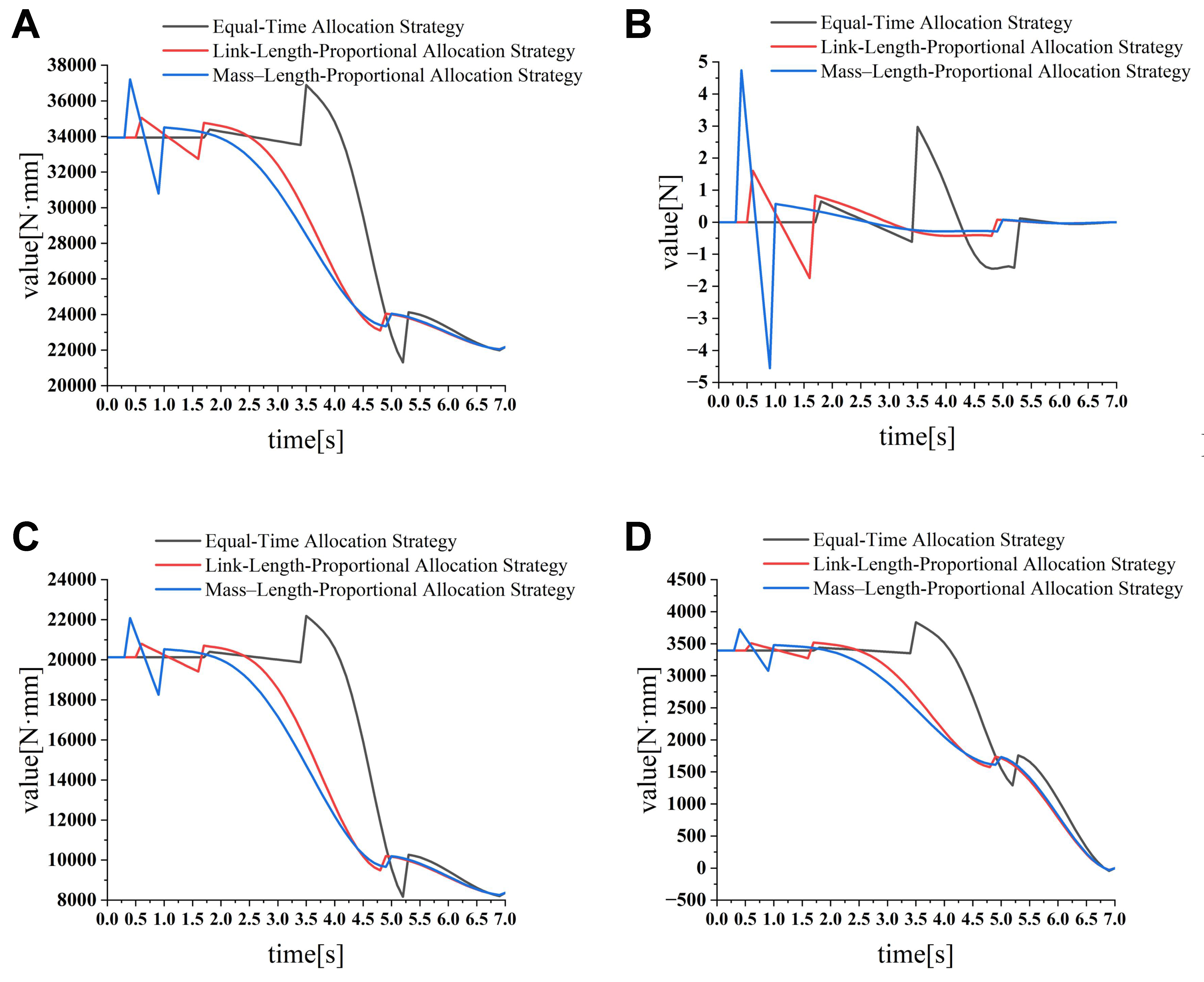
Figure 10. Joint force/torque comparison of each link under different allocation strategies: (A) rotating secondary arm; (B) translational arm; (C) picking main arm; and (D) picking secondary arm.
Using the amplitude and duration of the force/torque fluctuations as evaluation indices, the responses shown in Figure 10A were compared for the three predefined joint-time allocation strategies. During the first half of the motion cycle (0-3.5 s), the mass–length-proportional allocation strategy exhibits the largest peak-to-peak variation in force/torque. In particular, a pronounced abrupt change occurs between 0.5 and 1.0 s, indicating stronger transient fluctuations than those produced by the other two strategies. During the second half of the motion cycle (3.5-7.0 s), the equal-time allocation strategy shows the largest peak-to-peak variation, characterized by a sharp spike at approximately 3.75 s followed by a rapid decline. By comparison, the link-length-proportional allocation strategy exhibits relatively moderate force/torque fluctuation amplitudes and avoids the pronounced transient variations observed under the mass–length-proportional and equal-time strategies. At 7.0 s, the torque responses of all three strategies converge to the same steady-state value of approximately
The differences among the three strategies can be attributed to their respective joint-time distributions. Under the mass–length-proportional allocation strategy, relatively short motion durations are assigned to the secondary rotational joint and the translational joint, resulting in comparatively large initial force/torque peaks. The equal-time allocation strategy produces a pronounced abrupt variation during the later stage of the motion cycle. In contrast, the link-length-proportional allocation strategy avoids the largest transient peaks observed in the other two strategies and provides a comparatively smooth actuator-load response under the prescribed boundary-point trajectory. Accordingly, it was selected for the subsequent payload-dependent analysis, motion-cycle analysis, simulations, and physical experiments. This selection represents an engineering choice among the three predefined allocation strategies under the tested trajectory and operating conditions. Because the allocation ratios were specified in advance and no numerical search or formal optimization procedure was employed, the comparison does not demonstrate local or global mathematical optimality.
5.2. Analysis under different payload conditions
The influence of varying loads on the dynamic characteristics of the picking mechanism is systematically investigated. Based on a link-length proportional optimization strategy, the joint motion time allocation is obtained, and simulations under different load cases are performed. The simulation process is divided into an outward reaching phase (0-7 s) and a return phase (7-14 s), with a total duration of 14 s. The payload-dependent simulation consists of a 7 s outward-reaching phase and a 7 s return phase, for a complete out-and-return simulation cycle of 14 s. The 14 s duration is a reciprocating simulation interval and does not represent the field single-fruit picking time.
In accordance with the actual single-fruit picking procedure, the joint motion ranges and time allocation are specified as listed in Table 11.
Single-step motion parameters of each link in the picking mechanism
| Parameter | Rotating secondary arm | Translational arm | Picking main arm | Picking secondary arm |
| Motion time | 0.54 s | 1.08 s | 3.23 s | 2.15 s |
| Motion velocity | 83.33 °/s | 92.59 mm/s | 18.58 °/s | 13.95 °/s |
| Motion range | 45° | 100 mm | 60° | 30° |
The picking mechanism is a serial structure, and the joints complete the entire single-fruit harvesting process sequentially. To simulate the end-effector load after fruit picking and ensure consistency with field operating conditions, equivalent additional loads of 0 kg (no load), 0.25 kg (light load), and 0.5 kg (full load) are applied at the gripper at t = 7 s. The load acts vertically downward and moves synchronously with the links.
To study how varying loads affect the driving joints, a 14 s complete working cycle is selected for analysis. The joint responses are examined over the entire motion period (0-14 s) under an identical trajectory, and the maximum forces and torques for different load conditions are summarized in Table 12.
Peak comparison of joint driving forces (torques) under different load conditions
| Load | Rotating secondary arm | Translational arm | Picking main arm | Picking secondary arm | ||||
| Maximum / N·mm | Minimum / N·mm | Maximum / N | Minimum / N | Maximum / N·mm | Minimum / N·mm | Maximum / N·mm | Minimum / N·mm | |
| 0 kg | 35,186.86 | 22,026.27 | 1.8096 | -1.776 | 20,875.26 | 8,234.37 | 3,524.32 | -45.9289 |
| 0.25 kg | 37,484.96 | 22,026.27 | 3.5773 | -1.776 | 22,643.03 | 8,234.37 | 4,395.16 | -45.9289 |
| 0.5 kg | 40,307.20 | 22,026.27 | 5.2744 | -1.776 | 25,028.67 | 8,234.37 | 5,355.16 | -45.9289 |
As shown in Figure 11, the picking mechanism operates under no-load conditions during 0-7 s, during which the joint force (torque) curves corresponding to the three preset loads completely overlap. This indicates that, in the absence of load, the joint dynamic characteristics are governed solely by kinematic constraints and are independent of the preset load parameters.
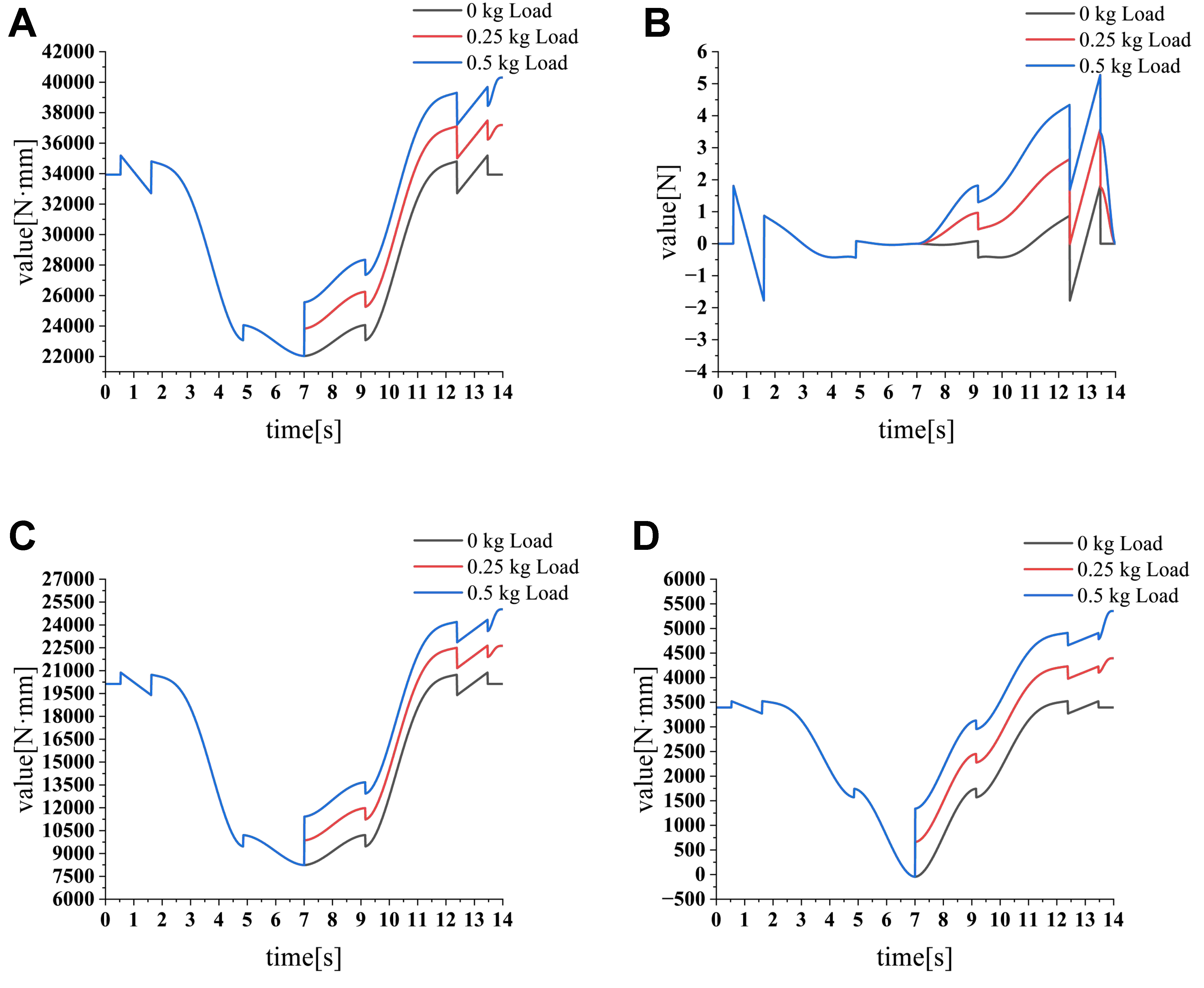
Figure 11. Joint dynamic parameters under different loads over the full time period. (A) Joint torque of the rotating secondary arm; (B) Joint force of the translational arm; (C) Joint torque of the picking main arm; (D) Joint torque of the picking secondary arm.
At t = 7 s, a sudden application of load causes a transient fluctuation in all curves. If this instantaneous disturbance is neglected, the variation patterns of the curves during 7-14 s remain consistent and symmetric with those observed during 0-7 s. This behavior is closely related to the symmetry of the motion trajectory and the sequential symmetry of joint motions in the serial mechanism.
As shown in Table 12, when the load increases from 0 to 0.5 kg, the differences in the maximum joint forces (torques) are 5,120.34 N·mm, 3.4648 N, 4,153.41 N·mm, and 1,830.84 N·mm, respectively. To analyze the influence of the maximum force (or torque) on the joint mechanical characteristics and eliminate the effect of dimensionality, a normalized secant load-response index (χ) is introduced to compare the finite change in the maximum joint response over the tested payload interval.
where m0, m0.25, and m0.5 denote the load masses, with values of 0, 0.25, and 0.5, respectively. In the equation, D0 represents the maximum joint force (torque) under a 0 kg load; D0.25 represents the maximum joint force (torque) under a 0.25 kg load; and D0.5 represents the maximum joint force (torque) under a 0.5 kg load. The index χ represents a normalized finite-difference response between the tested payload levels. It is not a local derivative or elasticity and should not be interpreted as the percentage response caused by a 1% infinitesimal change in payload.
According to Equation (39), the normalized secant load-response indices over the tested payload interval are 6.83% for the rotating secondary arm, 48.43% for the translational arm, 9.17% for the picking main arm, and 20.83% for the picking secondary arm. Among the four joints, the translational joint exhibits the largest normalized finite change between the three tested payload conditions.
These values are descriptive indices based on payloads of 0, 0.25, and 0.5 kg. They do not represent local elasticities, and 48.43% must not be interpreted as indicating that a 1% payload change causes a 48.43% change in force.
Because the payload is applied as a step input at t = 7 s, the reported global maxima may include both the transient impact of load application and the subsequent loaded motion response. A more detailed separation of static and transient load effects will require additional payload levels and dedicated regression experiments.
Over the three tested payload levels, the translational joint exhibited the largest normalized secant change in maximum actuator load. This result provides a qualitative indication that the translational drive deserves particular attention in actuator selection. The reported index is not interpreted as a local payload elasticity.
5.3. Analysis under different motion cycle conditions
Three representative simulation durations of 14 s, 18 s, and 22 s are adopted to examine the effect of different motion cycles on the kinematic behavior of the picking mechanism. In this section, “simulation cycle” refers specifically to the complete out-and-return reciprocating simulation duration. Three complete simulation cycles of 14, 18, and 22 s are evaluated. For each test group, the motion time of each step is reduced by 0.5 s relative to the previous group, and comparative experiments are conducted under identical loading conditions. To ensure comparability across tests, a constant working load of 0.25 kg was applied in all cases, so that differences in the motion response of the mechanism could be attributed to the tested motion parameters rather than variations in load.
In contrast to the boundary-reaching trajectories used in Sections 5.1 and 5.2, Section 5.3 employs a fixed reciprocating trajectory to investigate the sensitivity of the mechanism response to motion-cycle duration. The prescribed motion ranges are 30° for the rotating secondary arm, 24 mm for the translational arm, 22.5° for the picking main arm, and 45° for the picking secondary arm. These ranges remain unchanged across the three simulated cycle-duration conditions, with only the corresponding motion durations being varied. This controlled setup isolates the effect of motion-cycle duration from that of joint displacement, thereby enabling the influence of cycle duration on the motion and dynamic responses of the mechanism to be systematically evaluated. Accordingly, the analysis is intended to reveal the response characteristics associated with different motion-cycle durations under a prescribed trajectory rather than to reproduce the full boundary-reaching trajectories reported in Tables 9 and 11. The specific simulation parameters are summarized in Table 13.
Single-step motion parameters of each link and total simulation time
| Group | Name | Range | ||||
| Single-link motion time | Single-link motion velocity | Single-link motion | Single-step simulation time | Total simulation time | ||
| 1 | Rotating secondary arm | 2 s | 15°/s | 30° | 11 s | 22 s |
| Translational arm | 3 s | 8 mm/s | 24 mm | |||
| Picking main arm | 3 s | 7.5°/s | 22.5° | |||
| Picking secondary arm | 3 s | 15°/s | 45° | |||
| 2 | Rotating secondary arm | 1.5 s | 20°/s | 30° | 9 s | 18 s |
| Translational arm | 2.5 s | 9.6 mm/s | 24 mm | |||
| Picking main arm | 2.5 s | 9°/s | 22.5° | |||
| Picking secondary arm | 2.5 s | 18°/s | 45° | |||
| 3 | Rotating secondary arm | 1 s | 30°/s | 30° | 7 s | 14 s |
| Translational arm | 2 s | 12 mm/s | 24 mm | |||
| Picking main arm | 2 s | 11.25°/s | 22.5° | |||
| Picking secondary arm | 2 s | 22.5°/s | 45° | |||
Based on its motion characteristics, the dynamic parameters of the translational arm, the picking main arm, and the picking secondary arm are analyzed [Figure 12].
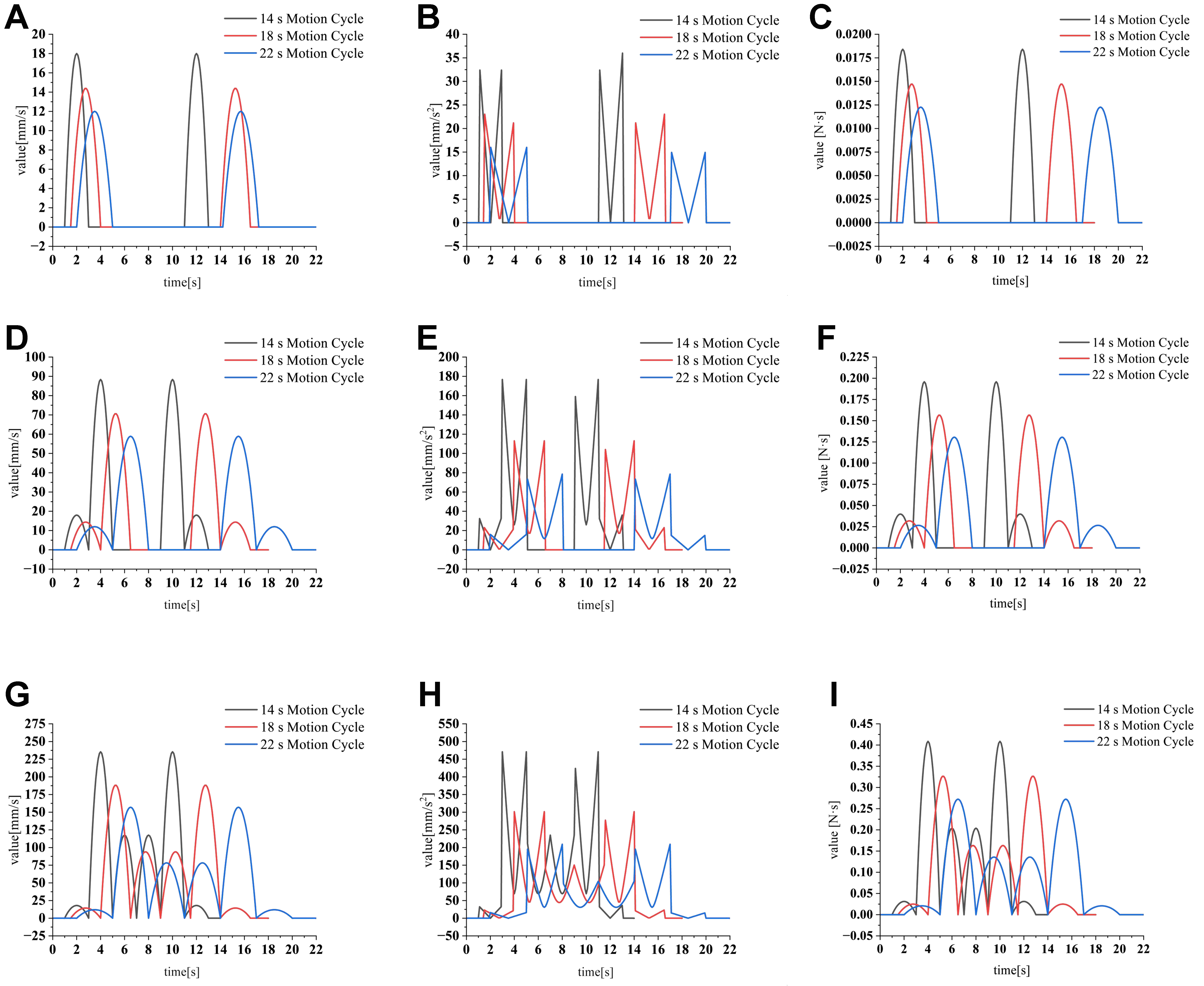
Figure 12. Joint dynamic parameter curves of the picking mechanism. (A) Centroid velocity of the translational arm; (B) Centroid acceleration of the translational arm; (C) Momentum of the translational arm; (D) Centroid velocity of the picking main arm; (E) Centroid acceleration of the picking main arm; (F) Momentum of the picking main arm; (G) Centroid velocity of the picking secondary arm; (H) Centroid acceleration of the picking secondary arm; (I) Momentum of the picking secondary arm.
As shown in Figure 12, the motion parameter curves of each joint exhibit an approximately symmetric distribution about the midpoint of the motion cycle, which is highly consistent with the temporal characteristics of the “out-and-return” reciprocating motion in the picking operation. When the centroid velocity reaches its maximum value, the momentum simultaneously attains its peak. The maximum values occur at the picking secondary arm during the 14 s motion cycle, as shown in Figure 12G-I, with values of 235.47 mm/s, 470.94 mm/s², and 0.41 N·s, respectively. From Figure 12A, B, D, E, G, and H, it can be further observed that as the complete out-and-return simulation cycle is shortened from 22 to 14 s, the peak centroid velocity and acceleration increase correspondingly.
These results reveal the intrinsic coupling relationship among motion cycle, dynamic parameters (velocity, acceleration, and momentum), and system vibration. This provides a theoretical basis and engineering guidance for subsequent optimization of structural stability and vibration suppression of the picking mechanism.
6. METHODS
6.1. Software and computational implementation
The kinematic and dynamic calculations were performed using MATLAB R2022b (MathWorks, Natick, MA, USA). The multibody dynamic model was established and solved using MSC Adams 2021 (MSC Software Corporation, USA), and the three-dimensional mechanical model was prepared using SolidWorks 2020 (Dassault Systèmes, France). The robot-control and data-transfer programs were implemented using Python 3.10.9. The recorded high-speed images were processed using TEMA Motion 2022 (Image Systems AB, Sweden). All analyses were performed on a Lenovo ThinkBook computer equipped with an Intel Core i7-12700H processor, 32 GB of RAM, and the 64-bit Windows 10 operating system.
6.2. Boundary-point tracking experiment
The boundary-point tracking experiment was conducted on an open hard-ground test site at the Agricultural Experimental Station of Shandong Agricultural University in June 2025. The open site was selected to minimize interference from uneven orchard terrain, branches, foliage, wind-induced fruit motion, and variable canopy occlusion, thereby facilitating stable observation of the prescribed reference-point trajectories. The experiment was designed to evaluate the motion-execution accuracy of the picking mechanism under controlled conditions while avoiding interference from orchard terrain and environmental variability. The planar tracking errors were calculated from the deviations between the measured and theoretical coordinates in the calibrated Y–Z measurement plane. Because the present single-view arrangement did not provide independently calibrated depth information along the X-axis, a complete three-dimensional Euclidean error was not calculated. The high-speed camera was positioned approximately perpendicular to the Y–Z measurement plane and was used to track the marker corresponding to the gripper reference point. The inclinometer and laser displacement sensor measured the revolute-joint angles and prismatic-joint displacement, respectively. The purpose of this experiment was to evaluate boundary-reference-point reaching accuracy, joint-motion accuracy, and arrival-time accuracy under controlled measurement conditions. No fruit-contact or fruit-detachment criterion was involved in this experiment. The experiment was conducted using the developed harvesting robot, which was equipped with a Lenovo ThinkBook laptop, a VEO410L high‑speed camera (York Technology Co., Beijing; 1280 × 800 resolution, 5200 fps, 190 μs exposure), a DL1903 inclinometer (0.05° accuracy), an HG‑C1100 laser displacement sensor (0.01 mm accuracy; Panasonic, Japan), a handheld temperature and humidity meter (0.1 °C accuracy), a vernier caliper, a measuring tape, a stopwatch, and related auxiliary equipment.
6.3. Orchard harvesting experiment
The orchard harvesting experiment was conducted in October 2025 at the orchard experimental base of the Horticulture Experimental Station of Shandong Agricultural University to evaluate the harvesting performance of the robot under actual orchard conditions. The experimental orchard was planted with ‘Golden Delicious’ apple trees. The average intra-row spacing and inter-row spacing were approximately 2.0 and 3.0 m, respectively. The measured inter-row spacing of approximately 3.0 m falls within the robot’s specified applicable inter-row operating range of 2.5-3.5 m. The intra-row spacing of approximately 2.0 m represents the actual spacing between adjacent trees in the experimental orchard and is not a machine operating-range parameter. The mean tree height was approximately 3.1 m, and the mean canopy diameter was approximately 1.6 m. The orchard terrain was relatively flat, providing suitable operating conditions for the mobile harvesting platform.
Before the experiment, the robot was positioned between adjacent tree rows and operated using the joint-motion parameters selected from the preceding motion-parameter allocation analysis. Apples located within the effective picking regions of the robot were selected as harvesting targets. For each target, the positioning mechanism first moved the picking mechanism to the corresponding operating region, after which the picking mechanism executed the prescribed reaching, grasping, and detachment motions. A harvesting attempt was defined as successful when the target apple was detached from the tree and securely retained by the end-effector after completion of the picking operation.
The harvesting performance was evaluated using two indicators: picking success rate and single-fruit picking time. The picking success rate was calculated as the ratio of the number of successfully harvested apples to the total number of attempted targets. The single-fruit picking time was defined as the elapsed time required to complete one fruit-picking operation and was recorded for each tested picking region. The orchard experiment was intended to evaluate the practical harvesting performance of the robot under the tested orchard conditions and was not used to quantify geometric tracking errors.
Descriptive variability among the ten tested orchard domains was quantified using the population standard deviation,
where n = 10 is the total number of experimental domains included in the field campaign. The coefficient of variation was calculated as
Population rather than sample standard deviation was used because these statistics were intended to descriptively characterize the complete set of domains tested in the present experimental campaign.
7. EXPERIMENTAL VALIDATION AND RESULTS ANALYSIS
7.1. Experimental methods and conditions
7.1.1. Planar boundary-point tracking experiment in the Y–Z measurement plane
Following the Agricultural Machinery Production Test Methods (GB/T 5667–2008)[31], a high-speed-camera-based tracking experiment was conducted at predefined boundary reference points within the picking domain. A marker located at the gripper reference point was tracked to evaluate the planar reaching accuracy of the gripper and the execution accuracy of the selected joint-motion parameters.
The experiment was performed on an open hard-ground site at the Agricultural Experimental Station of Shandong Agricultural University to avoid interference from orchard terrain and complex environmental conditions and to ensure full trajectory capture of the reference point. A high-speed camera was employed, and the setup is shown in Figure 13. The experiment was completed in June 2025.
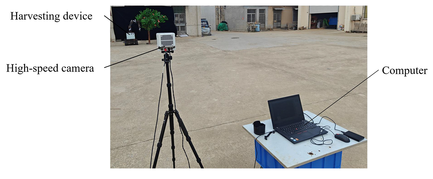
Figure 13. Experimental setup for boundary reference point tracking. Photograph taken by the authors.
Based on the selected joint-motion parameters, the joint velocities were set to drive the joints to rotate toward the boundary reference point of the picking domain [Figure 14]. For each reference point, 10 repeated trials were conducted. Under the X0Y0Z0 coordinate frame, the coordinates of the boundary reference point were measured, and the time required to reach the target in each trial was recorded.
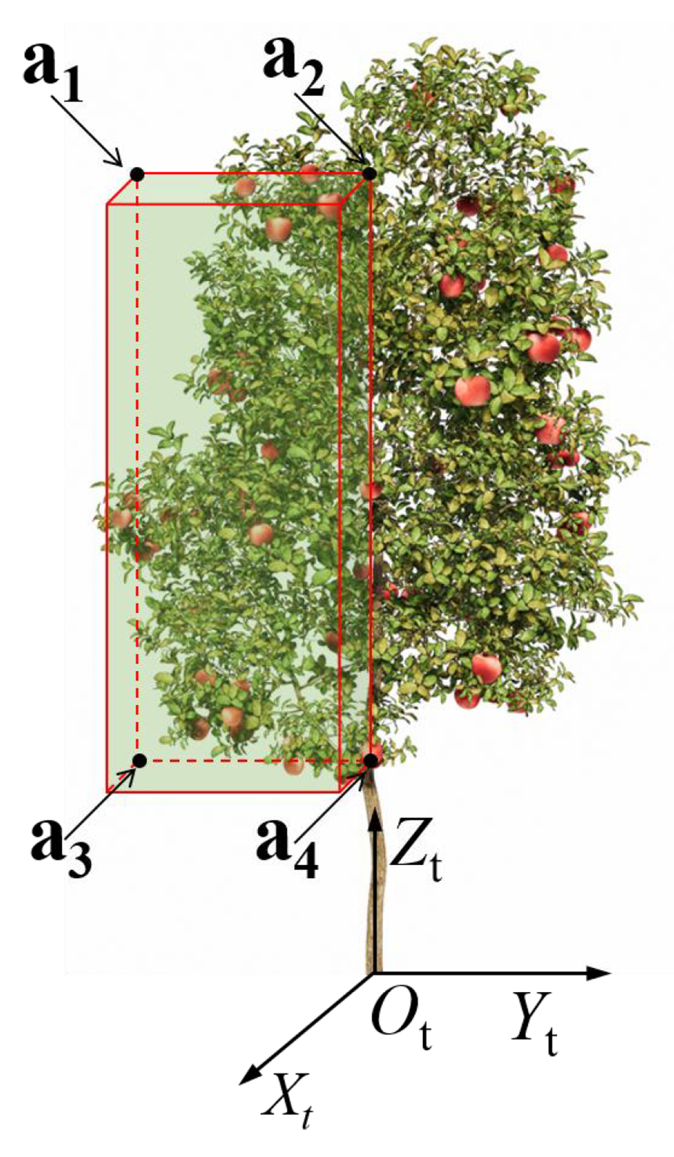
Figure 14. Boundary reference points of the target picking domain.
The camera was positioned approximately perpendicular to the Y–Z measurement plane, and the image scale was calibrated using a reference length located in the same plane as the tracked marker. Accordingly, the camera data were used solely to evaluate the planar Y- and Z-coordinates rather than to reconstruct the full three-dimensional position. The joint sensors and camera were triggered by the same motion command to ensure temporal synchronization, and the arrival time was determined from the recorded motion sequence. The camera resolution, frame rate, exposure time, inclinometer accuracy, and laser displacement sensor accuracy are reported above.
The boundary reference point trajectories are captured in the X0Y0Z0 coordinate frame from the positive X0Y0Z0 axis and the negative Y0 axis to obtain positional data. At the same time, joint angles θ4, θ6, θ7, and the displacement ex5 are synchronously measured using an inclinometer and a laser displacement sensor. The last-frame images of each reference point are shown in Figure 15.
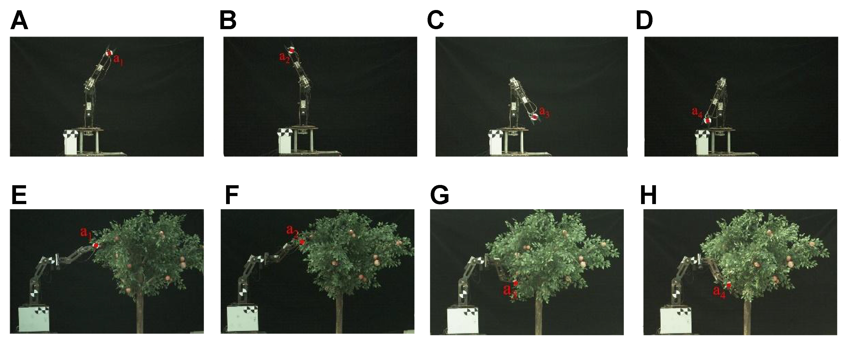
Figure 15. Final-frame images of reference points in the target picking domain under different axial directions. (A) Point a1 in the positive X0-axis direction; (B) Point a2 in the positive X0-axis direction; (C) Point a3 in the positive X0-axis direction; (D) Point a4 in the positive X0-axis direction; (E) Point a1 in the negative Y0-axis direction; (F) Point a2 in the negative Y0-axis direction; (G) Point a3 in the negative Y0-axis direction; (H) Point a4 in the negative Y0-axis direction. Photograph taken by the authors.
7.1.2. Orchard harvesting experiment
The picking experiments were conducted in October 2025 at the orchard experimental base of Shandong Agricultural University’s Horticulture Experimental Station, as shown in Figure 16. The experimental orchard had an average intra-row tree spacing of approximately 2.0 m and an inter-row spacing of approximately 3.0 m. Inter-row spacing primarily determines the available traveling corridor for the mobile platform, whereas the intra-row spacing describes the distance between adjacent trees and influences the longitudinal distribution of harvesting targets. Because the 3.0 m inter-row spacing falls within the robot’s specified applicable range of 2.5-3.5 m, the harvesting robot operated under suitable row-spacing conditions during the experiment.
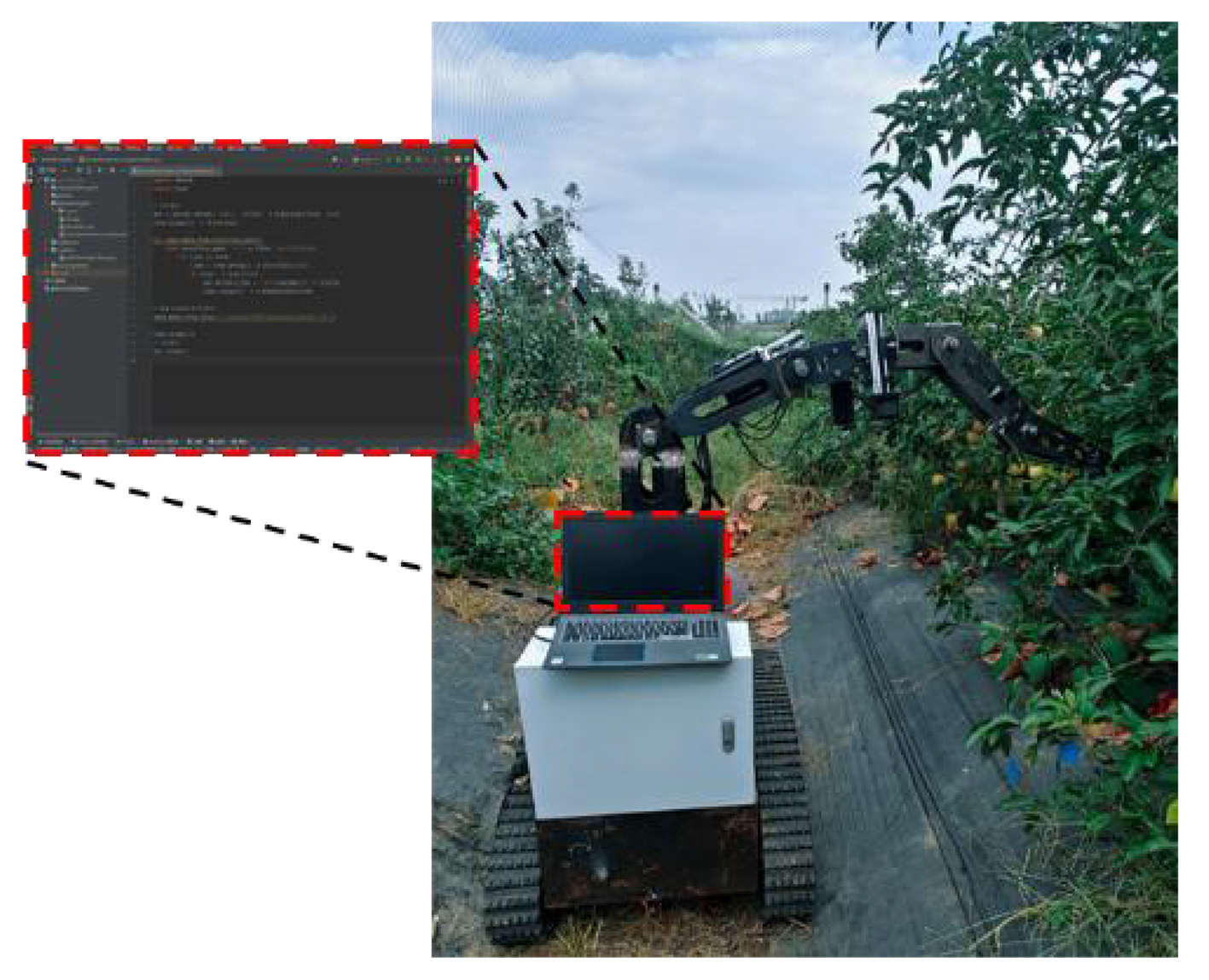
Figure 16. Picking performance test site. Photograph taken by the authors.
The average tree height was 3.1 m (± 0.2 m), and the canopy diameter was 1.6 m (1.5 m in the north–south direction and 1.7 m in the east–west direction). The ambient temperature during the experiment was 33 °C. The orchard terrain was flat, ensuring stable mechanical operation conditions. The orchard experiments evaluated harvesting performance, including successful picking rate and picking time. They were not used for calculating geometric tracking errors.
7.2. Experimental results and analysis
7.2.1. Position accuracy verification of boundary points in fruit trees
The images recorded by the high-speed camera were processed using TEMA image analysis software to obtain the actual coordinates of the boundary reference points, which were then compared with the theoretical values for validation.
The present single-view experimental arrangement was calibrated for the Y–Z measurement plane and did not provide independent stereoscopic depth reconstruction along the X-axis. Consequently, the present analysis is limited to Y- and Z-coordinate errors, and no claim is made of complete three-dimensional tracking accuracy.
These coordinates directly reflect the accuracy of the joint driving parameters. Validation results [Figure 17] were obtained by comparing the measured position data with the theoretical values. Planar tracking accuracy was evaluated component-wise using the absolute Y- and Z-coordinate errors defined in Section 6.2. Because the single-view camera arrangement did not provide independently calibrated X-direction depth information, a complete three-dimensional Euclidean error was not calculated.
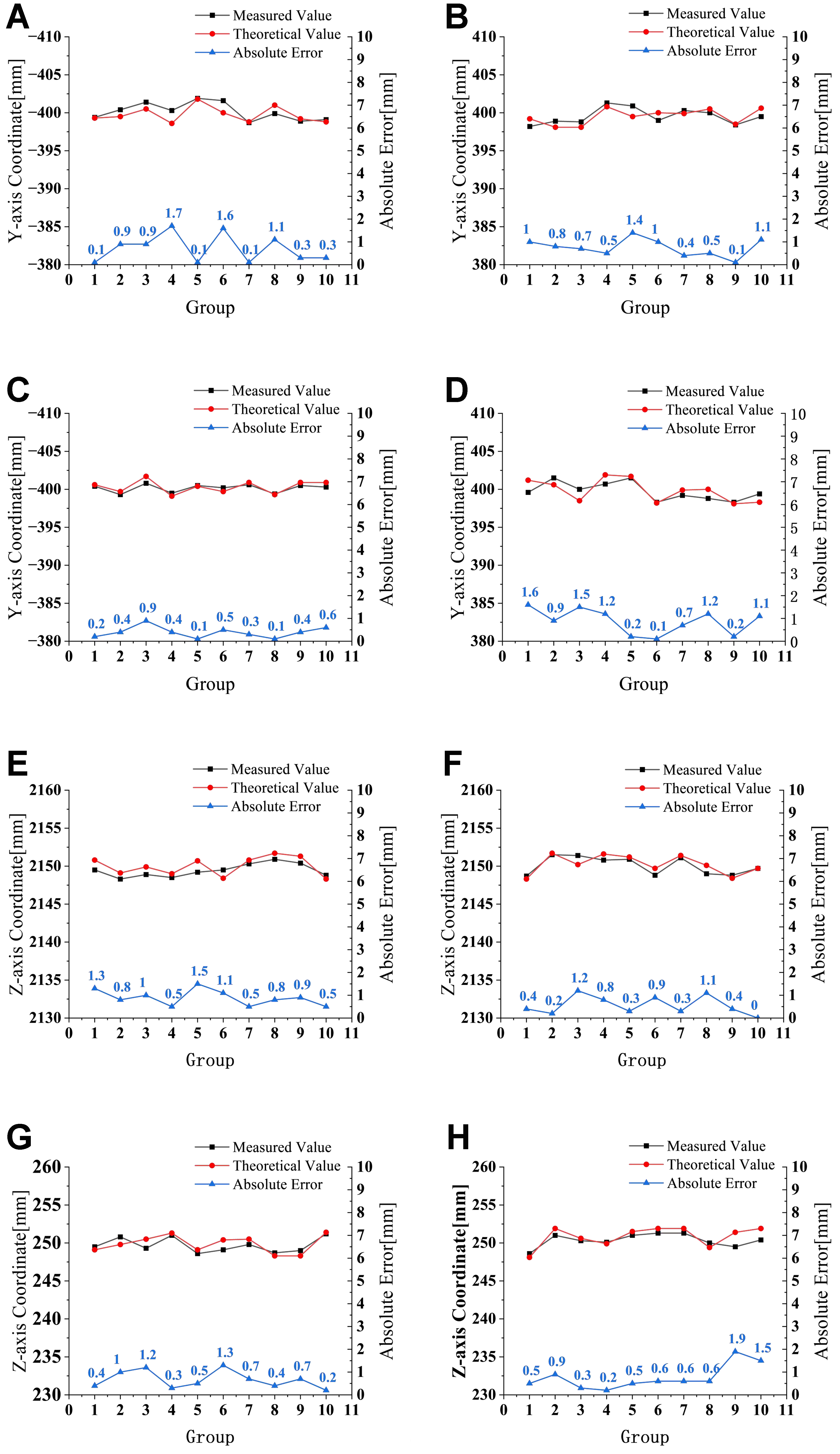
Figure 17. Comparison between measured and theoretical Y- and Z-axis coordinates of boundary reference points in the target picking region: (A-D) Y-axis coordinates of points a1-a4; (E-H) Z-axis coordinates of points a1-a4.
The present single-camera measurement system was calibrated for planar tracking in the Y–Z plane and did not provide independently calibrated depth reconstruction along the X-axis. As shown in Figure 17, the Y-direction errors at the four reference points were 1.7, 1.4, 0.9, and 1.6 mm, while the corresponding Z-direction errors were 1.5, 1.2, 1.3, and 1.9 mm, respectively. All measured errors were within the predefined picking-accuracy threshold of 2.0 mm, with maximum errors of 1.7 mm in the Y direction and 1.9 mm in the Z direction. These results demonstrate the tracking accuracy of the mechanism within the calibrated Y–Z measurement plane but should not be interpreted as a complete three-dimensional positioning assessment. Because the X-direction depth error and the three-dimensional Euclidean error could not be independently measured using the present single-view arrangement, future work will employ synchronized stereo cameras or an external three-dimensional tracking system to evaluate full spatial positioning error and coordinate-registration uncertainty.
7.2.2. Validation of the link-length proportional parameter scheme
Based on the conclusions of Section 5.1 regarding the positional accuracy of boundary reference points and the measured data, the accuracy of the selected joint-motion parameters (i.e., rotational angles and displacement distances) is further verified. Considering the symmetric characteristics of the picking domain, the joint rotation angles and displacement distances of each boundary reference point exhibit scalar consistency.
Taking the representative reference point a1 as an example, and using the calculated joint parameters in Table 9 as theoretical values, the absolute errors between the measured and theoretical values are calculated. The results are presented in Table 14. The distribution of absolute joint errors for the remaining reference points (a2-a4) is shown in Figure 18.
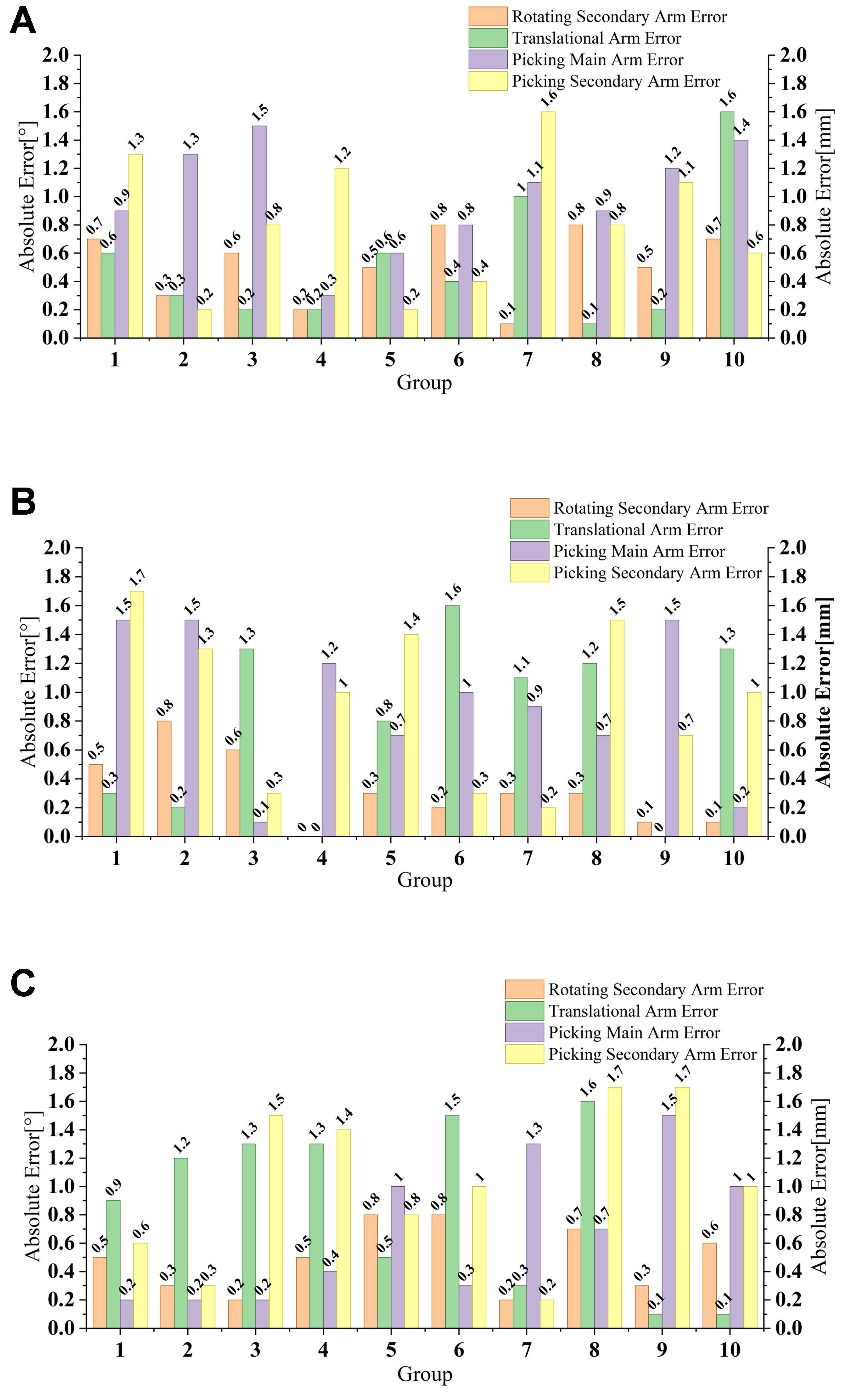
Figure 18. Absolute errors of joint rotation angles and displacement distances at reference points a2, a3, and a4. (A) Reference point a2; (B) Reference point a3; (C) Reference point a4.
Measured values and absolute errors of joint motion parameters at reference point a1
| Group | Rotating secondary arm | Translational arm | Picking main arm | Picking secondary arm | ||||
| Measured value /° | Absolute value /° | Measured value /mm | Absolute value /mm | Measured value /° | Absolute value /° | Measured value /° | Absolute value /° | |
| 1 | 44.9 | 0.1 | 100.3 | 0.3 | 60.7 | 0.7 | 29.6 | 0.4 |
| 2 | 45.1 | 0.1 | 100.2 | 0.2 | 59.5 | 0.5 | 30.3 | 0.3 |
| 3 | 45.2 | 0.2 | 100.4 | 0.4 | 60.7 | 0.7 | 29.9 | 0.1 |
| 4 | 45.1 | 0.1 | 99.7 | 0.3 | 60.5 | 0.5 | 30.6 | 0.6 |
| 5 | 44.6 | 0.4 | 99.8 | 0.2 | 60.7 | 0.7 | 29.7 | 0.3 |
| 6 | 44.9 | 0.1 | 99.3 | 0.7 | 60.2 | 0.2 | 30.1 | 0.1 |
| 7 | 45.2 | 0.2 | 99.5 | 0.5 | 59.8 | 0.2 | 29.7 | 0.3 |
| 8 | 45.5 | 0.5 | 100.5 | 0.5 | 60.3 | 0.3 | 30.7 | 0.7 |
| 9 | 45.4 | 0.4 | 100.6 | 0.6 | 59.9 | 0.1 | 29.6 | 0.4 |
| 10 | 44.5 | 0.5 | 99.6 | 0.4 | 60.4 | 0.4 | 30.3 | 0.3 |
As shown in Table 14 and Figure 18, the maximum absolute errors in rotational angle and translational displacement across the four reference points did not exceed 1.7° and 1.6 mm, respectively. These results indicate that the picking mechanism could accurately execute the prescribed joint motions and reach the target positions, supporting the execution accuracy of the selected joint-motion parameters.
To evaluate temporal accuracy, the prescribed one-way reaching duration of 7 s defined in Section 5.1 was used as the theoretical reference. The signed arrival-time error for each trial was calculated as the difference between the measured arrival time and the prescribed 7 s reaching duration.
Table 15 shows that the mean signed arrival-time errors at reference points a1-a4 were -0.11, -0.08, -0.06, and -0.10 s, respectively. The largest magnitude of the mean signed error was 0.11 s.
Measured arrival times and signed arrival-time errors at each boundary reference point
| Group | Reference point a1 | Reference point a2 | Reference point a3 | Reference point a4 | ||||
| Measured value / s | Error / s | Measured value / s | Error / s | Measured value / s | Error / s | Measured value / s | Error / s | |
| 1 | 6.8 | -0.2 | 7.3 | 0.3 | 7.1 | 0.1 | 6.8 | -0.2 |
| 2 | 7.1 | 0.1 | 6.9 | -0.1 | 6.9 | -0.1 | 7.1 | 0.1 |
| 3 | 6.9 | -0.1 | 6.7 | -0.3 | 7.1 | 0.1 | 6.7 | -0.3 |
| 4 | 6.7 | -0.3 | 6.8 | -0.2 | 7 | 0 | 6.5 | -0.5 |
| 5 | 7.1 | 0.1 | 7.1 | 0.1 | 6.9 | -0.1 | 6.6 | -0.4 |
| 6 | 6.7 | -0.3 | 6.7 | -0.3 | 6.8 | -0.2 | 7.1 | 0.1 |
| 7 | 6.8 | -0.2 | 6.7 | -0.3 | 7 | 0 | 7 | 0 |
| 8 | 6.9 | -0.1 | 7.1 | 0.1 | 6.7 | -0.3 | 7.3 | 0.3 |
| 9 | 6.7 | -0.3 | 7.1 | 0.1 | 6.8 | -0.2 | 6.8 | -0.2 |
| 10 | 7.2 | 0.2 | 6.8 | -0.2 | 7.1 | 0.1 | 7.1 | 0.1 |
| Mean error | -0.11 s | -0.08 s | -0.06 s | -0.1 s | ||||
The experimental results indicate that the joint-motion parameters selected using the link-length-proportional allocation strategy satisfy the multi-dimensional accuracy requirements of orchard harvesting, including rotation angle, displacement, position, and time errors.
This validates the reliability of the optimized motion parameters in dynamic execution and provides essential support for precise and efficient operation of the picking mechanism.
7.2.3. Analysis of picking test results
From the experimental results, the single-domain picking success rate ηs is evaluated, and it can be expressed as:
Nsuccess refers to the count of successfully harvested fruits within one picking domain, and Ngoal is the total number of fruits in that domain.
As shown in Table 16, 287 of the 371 target apples were successfully picked across the ten test domains, corresponding to a pooled success proportion of 77.36% with an unadjusted Wilson 95% confidence interval of 72.83%-81.32%. The arithmetic mean of the ten domain-specific success rates was 77.38%; the slight difference from the pooled proportion results from variation in the number of target fruits among domains. Although the domain-level results were broadly consistent under the tested orchard and operating conditions, a success rate of approximately 77% remains below the level required for reliable autonomous deployment. Therefore, these experiments should be interpreted as a feasibility evaluation of the two-stage mechanism and the selected motion-parameter configuration rather than as evidence of mature operational reliability. The observed failures were mainly associated with branch interference and wind-induced fruit motion, which could not be actively compensated for by the current target-coordinate-based motion-execution system. The mean field single-fruit picking time was 6.94 s per fruit. Ref.[22] reported a historical mean of 7.24 s for an earlier experimental campaign using the same platform, corresponding to a descriptive reduction of approximately 4.09%. However, because the two datasets were not obtained through a contemporaneous randomized controlled comparison, this difference cannot be attributed solely to the joint-time allocation strategy.
Picking test results
| Group | Number of fruits in single domain / pcs | Number of successfully picked fruits / pcs | Picking success rate / % | Average single-fruit picking time / s |
| 1 | 35 | 27 | 77.14 | 6.91 |
| 2 | 37 | 28 | 75.68 | 6.84 |
| 3 | 40 | 31 | 77.50 | 7.12 |
| 4 | 38 | 30 | 78.95 | 6.94 |
| 5 | 32 | 25 | 78.13 | 7.05 |
| 6 | 41 | 31 | 75.61 | 6.81 |
| 7 | 37 | 29 | 78.38 | 6.79 |
| 8 | 39 | 30 | 76.92 | 7.15 |
| 9 | 35 | 27 | 77.14 | 6.87 |
| 10 | 37 | 29 | 78.38 | 6.96 |
| Arithmetic mean of domain-level results | 77.38 | 6.94 | ||
| Standard deviation | 1.07 | 0.12 | ||
| Coefficient of variation | 1.38% | 1.73% | ||
| Pooled result | 77.36% | |||
| Unadjusted Wilson 95%CI | 72.83%-81.32% | |||
The population standard deviation and coefficient of variation of the domain-level mean picking times were 0.12 s and 1.73%, respectively, indicating relatively low temporal dispersion across the ten tested domains. During the experiments, the 84 failed harvesting attempts were classified into three categories based on the available experimental records. Among them, 57 failures (67.86%) were attributed to branch obstruction or mechanical interference between the gripper and branches, and 11 failures (13.10%) were associated with wind-induced motion of the fruit or branches. The remaining 16 failures (19.05%) could not be reliably assigned to either category because of insufficient evidence or unclear causes. Therefore, branch-related mechanical interference was the predominant identifiable failure mode, followed by wind-induced target motion.
The pooled harvesting success rate of the present system was 77.36% (287 successful picks among 371 targets; 95% Wilson confidence interval: 72.83%-81.32%). This performance is comparable to the 76.97% success rate and 7.29 s average picking time reported for a dual-arm apple-harvesting robot by Huang et al.[32]. It falls within the range reported by Zhang et al.[33] who obtained success rates of 82.4% and 65.2% under different orchard structures with an average cycle time of approximately 6 s. More recently, Zhu et al.[34] reported success rates of 80.7% and 79.7% and an average picking cycle of 5.97 s in two commercial orchards. These comparisons indicate that the present system performs within the range of recent field-tested apple-harvesting robots, although its success rate remains lower than that of the best-performing recent systems. Direct ranking should nevertheless be treated cautiously because orchard architecture, fruit accessibility, end-effector design, and the definition of a successful cycle differ among studies.
8. CONCLUSIONS
(1) A kinematic model is developed by integrating the planting standards and agronomic requirements of dwarf high-density apple orchards with the geometric structure and motion characteristics of the picking robot. Singular configurations of the two mechanisms are analyzed based on the Jacobian matrix. The positioning mechanism shows no kinematic singularity, while the picking mechanism exhibits kinematic singularity at its initial configuration. Dynamic models of the positioning and picking mechanisms are developed based on their structural and kinematic characteristics, using the Lagrangian and Newton–Euler methods, respectively. The analytical dynamic model was numerically cross-verified against the ADAMS multibody model under matched assumptions. The results show that the mean relative errors of each link are 0.00152%, 0.598%, and 0.0856%, respectively, all less than 0.6%. The linear correlation coefficients between the theoretical and simulated joint curves are 0.999375, 0.999998, and 0.999999, indicating close numerical agreement between the two models.
(2) Under a fixed one-way reaching duration of 7 s, three predefined joint-time allocation strategies - equal-time, link-length-proportional, and mass–length-combined allocation - were comparatively evaluated using the established dynamic model. The force and torque fluctuation characteristics obtained under the prescribed boundary trajectory were used as engineering evaluation criteria. Among the three tested strategies, the link-length-proportional allocation exhibited comparatively moderate fluctuations and a relatively smooth and balanced actuator-load response, without the pronounced transient variations observed under the other two strategies. It was therefore selected for the subsequent payload-dependent and motion-cycle analyses, simulations, and physical experiments. The corresponding joint velocities were 83.33°/s, 92.59 mm/s, 18.58°/s, and 13.95°/s. This selection represents a preferred engineering configuration within the three predefined allocation strategies and the tested operating conditions. Because no numerical search or formal optimization procedure was performed, the result should not be interpreted as a mathematically proven local or global optimum.
(3) Boundary-reference-point tracking tests yielded maximum measured errors of 1.7 and 1.9 mm in the Y and Z directions, respectively, while the mean arrival-time error did not exceed 0.11 s. In the orchard field campaign, 287 of 371 target apples were successfully picked, corresponding to a pooled success rate of 77.36%, with a mean domain-level picking time of 6.94 s per fruit. These results support the feasibility of the proposed two-stage mechanism and the selected motion-parameter configuration under the tested conditions; however, they should not be interpreted as evidence of mature operational reliability or of a causal performance improvement, because no contemporaneous randomized baseline group was included. The observed failures were mainly associated with branch interference, wind-induced fruit motion, and the lack of online perception and adaptive obstacle-avoidance capabilities.
Based on the available experimental records, the 84 failed harvesting attempts were classified into three categories. Among them, 57 failures (67.86%) were attributed to branch obstruction or mechanical interference between branches and the gripper. Eleven failures (13.10%) were associated with wind-induced motion of the fruit or branches. The remaining 16 failures (19.05%) could not be reliably assigned to either category because of insufficient evidence, unclear causes, or the involvement of other factors. Therefore, branch-related mechanical interference was the predominant identifiable failure mode, followed by wind-induced target motion. Accordingly, the present study is limited to model-based motion generation and coordinated execution after a target coordinate has been provided, whereas fruit detection, multimodal sensor fusion, autonomous target selection, online obstacle avoidance, adaptive control, and autonomous decision-making remain outside the scope of the current experimental evaluation.
Future work will focus on two directions. First, agronomic–mechanical integration will be explored through manual canopy management, such as adjusting pruning angles and applying growth regulators, to improve branch spacing and reduce occlusion, thereby enhancing suitability for mechanized harvesting. Second, equipment adaptability will be addressed by addressing multi-target obstacle avoidance in dynamic environments through the integration of multimodal sensing technologies such as vision, force, and inertial navigation. A multi-angle, multi-pose approach strategy will be developed. By incorporating spatial distribution characteristics and intelligent path-planning algorithms, the system aims to enhance obstacle avoidance and improve harvesting success.
DECLARATION
Authors’ contributions
Conceptualization, methodology, software, investigation, writing: Yuan, B.
Validation, visualization, software, formal analysis: Fan, G.
Investigation, visualization: Ahn, H. S.; Pan, Y.
Visualization, software: Cao, X.
Writing - review and editing: Sun, L.
Investigation, visualization: Jing, L.
Conceptualization: Xue, L.; Liu, C. (Congning Liu); Liu, C. (Chunyang Liu)
Project administration, funding acquisition, resources: Zhang, H.; Wang, J.
All the authors approved the submitted manuscript.
Availability of data and materials
The datasets generated and analyzed during the current study, including experimental measurements, simulation results, and model parameters, are available from the corresponding author upon reasonable request. The source codes used for kinematic and dynamic calculations can also be provided for academic research purposes.
AI and AI-assisted tools statement
Not applicable.
Financial support and sponsorship
This work was supported by Shandong Province Key R&D Plan (Nos. 2023TZXD061 and 2025CXPT168); China Agriculture Research System (No. CARS-27); the National Natural Science Foundation of China (Youth Science Fund Project 32401723); the Young Talent of Lifting engineering for Science and Technology in Shandong (Nos. SDAST2024QTA050 and SDAST2025QTA048); the Shandong Province “University Youth Innovation Team” Program (No. 2023KJ160).
Conflicts of interest
All authors declared that there are no conflicts of interest.
Ethical approval and consent to participate
Not applicable.
Consent for publication
Not applicable.
Copyright
© The Author(s) 2026.
REFERENCES
1. National Bureau of Statistics of China, Department of Rural Social and Economic Survey. China Rural Statistical Yearbook 2024. http://www.tjcn.org/tjnj/NNN/43328.html. (accessed 2026-09-08).
2. Li, T.; Sun, J. M.; Huang, J. Z.; Lu, S. J. Fruit quality analysis and evaluation of ‘Fuji’ apples from different producing areas. J. China. Agric. Univ. 2024, 29, 23-9 (in Chinese).
3. Shang, S. Q.; Li, C. P.; He, X. N.; Wang, D. W.; Wang, H. Q.; Yang, S. Design and experiment of high-acid apple vibrating picker. Trans. Chin. Soc. Agric. Mach. 2023, 54, 115-25+68 (in Chinese).
4. Zhang, Z.; Igathinathane, C.; Li, J.; Cen, H.; Lu, Y.; Flores, P. Technology progress in mechanical harvest of fresh market apples. Comput. Electron. Agric. 2020, 175, 105606.
5. Luo, H.; Wei, G. System design and implementation of a novel robot for apple harvest. INMATEH-Agric. Eng. 2015, 46, 85-94. . (accessed 2026.
6. Zhang, K.; Lammers, K.; Chu, P.; Li, Z.; Lu, R. System design and control of an apple harvesting robot. Mechatronics 2021, 79, 102644.
7. Feng, Q.; Zhao, C.; Li, T.; et al. Design and test of a four-arm apple harvesting robot. Trans. Chin. Soc. Agric. Eng. 2023, 39, 25-33 (in Chinese).
8. Liu, J. Z.; Jiang, Y. X. Industrialization trends and multi-arm technology direction of harvesting robots. Trans. Chin. Soc. Agric. Mach. 2024, 55, 1-17 (in Chinese).
9. San, H. J.; Yang, X. Y.; Chen, J. P.; Wu, X. M.; Zhang, H. B.; Xu, B. Kinematic performance analysis and structural parameter optimization of delta parallel robot. Trans. Chin. Soc. Agric. Mach. 2024, 55, 446-58 (in Chinese).
10. Zhang, W. Z.; Feng, S. J.; Yuan, X. H.; Sun, P.; Yang, C.; Lu, Y. B. Kinematic analysis and optimization design of 2-PRU-PRRPa parallel mechanism. Trans. Chin. Soc. Agric. Mach. 2025, 56, 497-506 (in Chinese).
11. Huang, X.; Xiang, H.; Wu, C.; et al. CRAB-EDM: a multi-modal underwater crab-inspired robot with temporally sequenced electro-discharge modulation. IEEE. Robot. Autom. Lett. 2026, 11, 3939-46.
12. Li, B.; Wang, Q.; Yu, T.; et al. Quad-wing FWMAV with thrust vector yaw steering. Biomimetic. Intell. Robot. 2026, 6, 100327.
13. Zhou, Y. J.; Li, S. H.; Xu, Q.; Zhang, F. K. Kinematic analysis and optimal design of 3-PUS-PU compliant parallel mechanism. Trans. Chin. Soc. Agric. Mach. 2022, 53, 417-24 (in Chinese).
14. San, H. J.; Wu, X. M.; Chen, J. P.; Yang, X. Y.; Zhang, H. B. Kinematic analysis and parameter optimization of 5-DOF hybrid mechanism. Trans. Chin. Soc. Agric. Mach. 2025, 56, 701-12 (in Chinese).
15. Liu, X. F.; Liu, Y.; He, Y.; Wan, B.; Liu, Y.; Zhao, Y. S. Kinematic analysis and dimension optimization of multi-redundantly actuated parallel mechanism 2RPU+2UPR+RPR. Trans. Chin. Soc. Agric. Mach. 2023, 54, 440-50 (in Chinese).
16. Liu, S. H.; Wang, F.; Lin, M.; Liu, J. X.; Yao, K. H. Analysis and test of the kinematics characteristics of the robotic arm for a mango harvesting vehicle. Trans. Chin. Soc. Agric. Eng. 2024, 40, 58-67 (in Chinese).
17. Zhou, Y. J.; Wu, Q.; He, L. Y.; et al. Design and experiment of intelligent picking robot for famous tea. J. Mech. Eng. 2022, 58, 12-23 (in Chinese).
18. Zhao, X.; Cao, G. H.; Zhang, P. F.; Ma, Z. H.; Zhao, L. J.; Chen, J. N. Dynamic analysis and lightweight design of 3-DOF apple picking manipulator. Trans. Chin. Soc. Agric. Mach. 2023, 54, 88-98 (in Chinese).
19. Fu, M.; Guo, S.; Chen, A.; Cheng, R.; Cui, X. Design and experimentation of multi-fruit envelope-cutting kiwifruit picking robot. Front. Plant. Sci. 2024, 15, 1338050.
20. Wang, Z.; Pang, C.; Sui, J.; Zhao, G.; Wu, W.; Xu, L. Time-optimal trajectory planning for a six-degree-of-freedom manipulator: a method integrating RRT and chaotic PSO. Intell. Robot. 2024, 4, 479-502.
21. Li, Q.; Liu, E.; Cui, C.; Wu, G. An open-closed-loop iterative learning control for trajectory tracking of a high-speed 4-dof parallel robot. Intell. Robot. 2022, 2, 89-104.
22. Yuan, B.; Zhang, H.; Li, Y.; et al. Design and experimental evaluation of a two-stage domain-segmented harvesting device for densely planted dwarf apple orchards. AgriEngineering 2025, 7, 135.
23. Xue, X. M.; Chen, R.; Li, F. J.; Yu, S. Z.; Meng, C.; Yu, X. Y. High-quality and high-yield technology of super-dense cultivation of dwarf apple rootstock. China. Fruits. 2024, 101-4 (in Chinese).
24. Qiao, G. F.; Du, B. A.; Zhang, Y.; Tian, R. J.; Liu, D.; Liu, H. Z. Quadratic identification method of kinematic parameters of industrial robots based on POE model. Trans. Chin. Soc. Agric. Mach. 2024, 55, 419-25 (in Chinese).
25. Leng, S.; Wu, K.; Ju, H. H. Overview of manipulator kinematics modeling and solving method. J. Astronaut. 2019, 40, 1262-73 (in Chinese).
26. Zhao, Y. Z.; Liang, B. W.; Cao, Y. C.; Zhao, T. S. 3-PRRR translational parallel mechanism with constant jacobian matrix and its transfer performance analysis. Trans. Chin. Soc. Agric. Mach. 2017, 48, 333-8+67 (in Chinese).
27. Soltani, M.; Keshmiri, M.; Misra, K. A. Dynamic analysis and trajectory tracking of a tethered space robot. Acta. Astronaut. 2016, 128, 335-42.
28. Wang, H.; Liu, H. R.; Zou, S. Y.; Liu, Y. L. Research on dynamic modeling of SCARA robot with Gaussian process regression. Mach. Des. Manuf. , 2019, 235-7 (in Chinese).
29. Dong, X.; Wang, Z.; Guo, S. State estimation and attack reconstruction of picking robot for a cyber‐physical system. Math. Probl. Eng. 2022.
30. Tu, Q. Z.; Chen, Z. Y.; Pan, M.; Fang, Z. H. Dynamic modeling methods for 4-DOF serial bionic manipulator. J. Army. Eng. Univ. PLA. 2022, 1, 30-5 (in Chinese).
31. General Administration of Quality Supervision, Inspection and Quarantine of the People’s Republic of China, Standardization Administration of China. GB/T 5667-2008. Production test methods for agricultural machinery. 2008. https://www.chinesestandard.net/PDF/English.aspx/GBT5667-2008. (accessed 2026-09-08).
32. Huang, W.; Miao, Z.; Wu, T.; Guo, Z.; Han, W.; Li, T. Design of and experiment with a dual-arm apple harvesting robot system. Horticulturae 2024, 10, 1268.
33. Zhang, K.; Lammers, K.; Chu, P.; Li, Z.; Lu, R. An automated apple harvesting robot - from system design to field evaluation. J. Field. Robot. 2024, 41, 2384-400.
Cite This Article
 Open Access
How to Cite
Yuan, B.; Fan, G.; Ahn, H. S.; Pan, Y.; Cao, X.; Sun, L.; Jing, L.; Xue, L.; Liu, C.; Liu, C.; Zhang, H.; Wang, J. Motion analysis and parameter allocation of a two-stage apple-harvesting robot. Intell. Robot. 2026, 6(3), 582-620. https://dx.doi.org/10.20517/ir.2026.28
Download Citation
If you have the appropriate software installed, you can download article citation data to the citation manager of your choice. Simply select your manager software from the list below and click on download.
Export Citation File
Type of Import
Tips on Downloading Citation
Citation Manager File Format
Type of Import
Direct Import: When the Direct Import option is selected (the default state), a dialogue box will give you the option to Save or Open the downloaded citation data. Choosing Open will either launch your citation manager or give you a choice of applications with which to use the metadata. The Save option saves the file locally for later use.
Indirect Import: When the Indirect Import option is selected, the metadata is displayed and may be copied and pasted as needed.
About This Article
Special Topic
Copyright

Data & Comments
Data
0










Comments
Comments must be written in English. Spam, offensive content, impersonation, and private information will not be permitted. If any comment is reported and identified as inappropriate content by OAE staff, the comment will be removed without notice. If you have any queries or need any help, please contact us at [email protected].