


Suspension parameter identification method for rail transit vehicles using an AO-GRBF surrogate model and non-dominated sorting genetic algorithm
 0
0 Abstract
The suspension systems of rail transit vehicles are crucial components that connect the vehicle body to the wheelsets, designed to reduce vibrations and shocks induced by track irregularities. During extended service periods, suspension parameters such as stiffness and damping coefficients are inevitably altered due to material aging and temperature fluctuations, rendering vehicle control strategies based on original design values ineffective. This leads to increased vibrations, hunting instability, and potential safety hazards during operation. Therefore, a suspension parameter identification method is proposed that combines an adaptively optimized Gaussian radial basis function (AO-GRBF) surrogate model with the non-dominated sorting genetic algorithm II (NSGA-II) to address these challenges. First, a mechanism- and data-driven AO-GRBF model is constructed to approximate the nonlinear relationship between suspension parameters and vehicle vibration responses, thereby overcoming the high computational cost associated with conventional multibody dynamics models. Then, the NSGA-II algorithm is employed to identify optimal suspension parameters by minimizing the deviation between AO-GRBF surrogate predictions and field-measured responses. Validation using field measurements indicates that the proposed method outperforms existing approaches, such as the radial basis function-high-dimensional model representation (RBF-HDMR) method and the long short-term memory (LSTM) method, in terms of correlation and error metrics related to lateral and vertical vibration accelerations.
Keywords
1. INTRODUCTION
The suspension system connects the wheelsets to the vehicle body and is designed to attenuate shocks and vibrations induced by track irregularities [1,2]. Over time, suspension system parameters, such as stiffness and damping, deviate from nominal values due to in-service degradation and changes in operating conditions, including aging, thermal effects, and pneumatic variations[3,4]. This drift detunes vehicle control schemes that are preset to nominal design parameters and, in turn, exacerbates carbody vibration and hunting and may even increase safety risks, such as vehicle tilting during emergency braking [5,6]. Therefore, accurate identification of suspension parameters is essential to ensure operational safety and stability.
Suspension parameter identification has been investigated using both mechanistic and data-driven approaches. In mechanistic identification, high-fidelity simulation models of the suspension system are constructed, and advanced optimizers such as non-dominated sorting genetic algorithm II (NSGA-II) are employed for model-based parameter estimation to reliably search for values that best match in-service operating conditions [7,8]. Although physically interpretable results can be obtained, this approach requires substantial computational resources. To reduce this burden, data-driven surrogate models have been developed to replace the computationally expensive mechanistic models of the suspension system [9–16]. However, conventional surrogate models typically adopt static architectures and fixed sampling schemes, which limit their ability to capture localized nonlinearities and constrain accuracy in high-dimensional suspension parameter spaces [17–19]. Therefore, an identification framework that combines efficiency with accuracy is required.
In this study, an identification framework is proposed in which an adaptively optimized Gaussian radial basis function (AO-GRBF) surrogate is coupled with NSGA-II. First, a mechanistic train model is constructed to simulate suspension responses under different operating speeds, track conditions, and suspension parameter settings, thereby generating a physics-consistent training and validation dataset. Next, an AO-GRBF surrogate of the suspension system is built on this dataset, through adaptive resampling and kernel hyperparameter updates to improve local fidelity and to replace the computationally expensive mechanistic suspension model during the search. Finally, since suspension parameter identification is essentially a surrogate-based optimal-parameter search problem, NSGA-II is employed to explore the feasible set globally, avoid local optima, and obtain suspension parameter estimates close to their in-service values.
1.1. Novelty and contribution
Within the proposed AO-GRBF–NSGA-II framework, the principal contributions of this study are summarized as follows:
(1) To improve the stability of the GRBF surrogate model for suspension parameter identification under real operating conditions, an error-driven sampling mechanism is introduced to improve local fidelity in high-error regions. In addition, a multiobjective optimization scheme is employed to automatically adjust kernel-related parameters that determine model performance.
(2) To prevent convergence to local optima during parameter identification, a modified NSGA-II algorithm is adopted. This algorithm enables global search through population evolution combined with Pareto-based selection strategies.
(3) To demonstrate practical feasibility and deployment potential, the proposed method is validated using field-measured data obtained from rail transit operations.
The core technical challenge is to maintain accuracy and reliability when computationally intensive mechanistic models of suspension systems are replaced by data-driven surrogate models. This study addresses this challenge through residual-driven sampling, kernel self-tuning, and advanced evolutionary optimization.
1.2. Significance
Conventional approaches are constrained by lengthy offline computations, which limit the ability to detect suspension parameter variations in real time. As a result, early anomalies tend to be overlooked and the effectiveness of predictive maintenance is reduced. By contrast, the proposed method is designed to enable rapid parameter identification and timely detection of deviations, so that preventive actions can be taken before safety risks escalate. This advantage is expected to strengthen both railway safety and operational efficiency.
Beyond methodological innovation, the combined AO-GRBF and NSGA-II framework offers practical engineering benefits. First, an error-driven sampling strategy is employed to improve the robustness of the surrogate model to noise and non-stationary excitations, thereby ensuring stable performance under real operating conditions. Second, compared with repeated high-fidelity SIMPACK simulations, the surrogate-based approach significantly reduces computational cost. Consequently, efficient condition monitoring and predictive maintenance become more feasible in practical railway applications.
2. RELATED WORK
To provide a systematic background, existing methods for suspension parameter identification are reviewed, and their respective strengths and limitations are analyzed.
2.1. Mechanistic approaches
Mechanistic methods are based on nonlinear finite element (FE) or multibody dynamics (MBD) models of railway vehicles. These models are typically implemented on industrial platforms such as SIMPACK or Ansys to simulate system responses under parameter variations [7,8]. Suspension parameters are identified by solving an inverse problem in which discrepancies between simulated and measured responses are minimized [8]. For instance, Zhang et al. developed a mechanistic model for high-speed trains and determined stiffness and damping coefficients using a min-max method [6]. Yao et al. employed a simplified lateral dynamic model combined with NSGA for robust stability identification [20]. Kraft et al. formulated parameter identification as an adjoint-state inverse problem, which enabled accurate calibration [8]. Although these methods provide physically interpretable results, their high computational costs limit practical field applications [7,8,21,22].
2.2. Surrogate model-based approaches
To reduce computational costs, surrogate models such as Kriging, radial basis function (RBF), and neural networks have been employed to approximate the mapping from parameter inputs to suspension system performance responses; subsequently, these surrogates are coupled with optimization algorithms to identify parameter sets that best correspond to actual operating conditions [9–16].
Among these surrogates, RBF models are widely used for nonlinear black-box systems because they provide mesh-free interpolation with competitive accuracy and training cost in high-dimensional settings [23]. However, performance depends critically on the sampling policy: when constructed from static, one-shot designs, RBF surrogates tend to miss localized nonlinear dynamics, and accuracy degrades across the high-dimensional suspension parameter space [17–19]. To address these issues, adaptive RBF frameworks have been proposed. For example, Liu et al. introduced a trust-region-based adaptive RBF (TARBF) that sequentially enriches samples within moving trust regions to improve sample efficiency and local fidelity for computationally expensive constrained problems[18]. Ye et al. presented an RBF-assisted adaptive differential evolution (RBF-ADE) with a cooperative dual-phase infill strategy to accelerate convergence and enhance surrogate accuracy in high-dimensional expensive tasks[19]. Nevertheless, in both approaches, the basis-function class remains fixed, and kernel hyperparameters are not jointly optimized with the sampling policy. Moreover, direct integration of adaptive RBF surrogates into suspension parameter identification remains scarce, which limits their application under in-service conditions.
In addition, as suspension parameter identification is fundamentally a surrogate-based optimal-parameter search, the multiobjective evolutionary algorithm NSGA-II is commonly adopted to prevent premature convergence and maintain population diversity. For example, Zhang et al. developed a neural-network surrogate to replace computational fluid dynamics and vehicle-dynamics models under crosswind conditions and coupled it with NSGA-III to identify bogie suspension parameters [14]. Zhang et al. also established a deep-learning surrogate to approximate heavy-haul freight train dynamics and employed NSGA-II to estimate key longitudinal stiffness and damping coefficients [15]. Jiang et al. constructed surrogate models of parameterized suspension components and integrated them with NSGA-II for lightweight optimization [16].
2.3. Novelty of the proposed method
This study employs two key algorithms. First, a data-driven AO-GRBF surrogate is introduced to replace the computationally intensive mechanistic model of the suspension system while retaining fidelity under variable in-service conditions. Within AO-GRBF, residual-driven sampling and in-loop kernel updates operate in a closed loop to target difficult regions of the high-dimensional, nonlinear suspension parameter space. After each enrichment step, the kernel shape and regularization are updated to fit local curvature, improving local fidelity and preserving robustness as operating conditions drift.
Second, NSGA-II is employed to define a surrogate-based multiobjective optimization framework, converting parameter identification into a tractable model-optimization problem. Pareto-based global evolution maintains population diversity and conducts a reliable search across the suspension parameter space to balance accuracy and robustness, yielding estimates that best match actual operating conditions.
3. METHODS
The suspension system of a rail transit vehicle is selected as the research subject. Since stiffness and damping parameters are crucial to determine vehicle vibration responses to track excitations, vehicle body vibration acceleration is selected as the evaluation metric for parameter identification. A data-driven AO-GRBF surrogate model is constructed to approximate the nonlinear mapping relationship between suspension parameters and vibration responses, which enables faster parameter identification. Subsequently, NSGA-II is employed to identify the optimal suspension parameter combination that best matches measured dynamic responses.
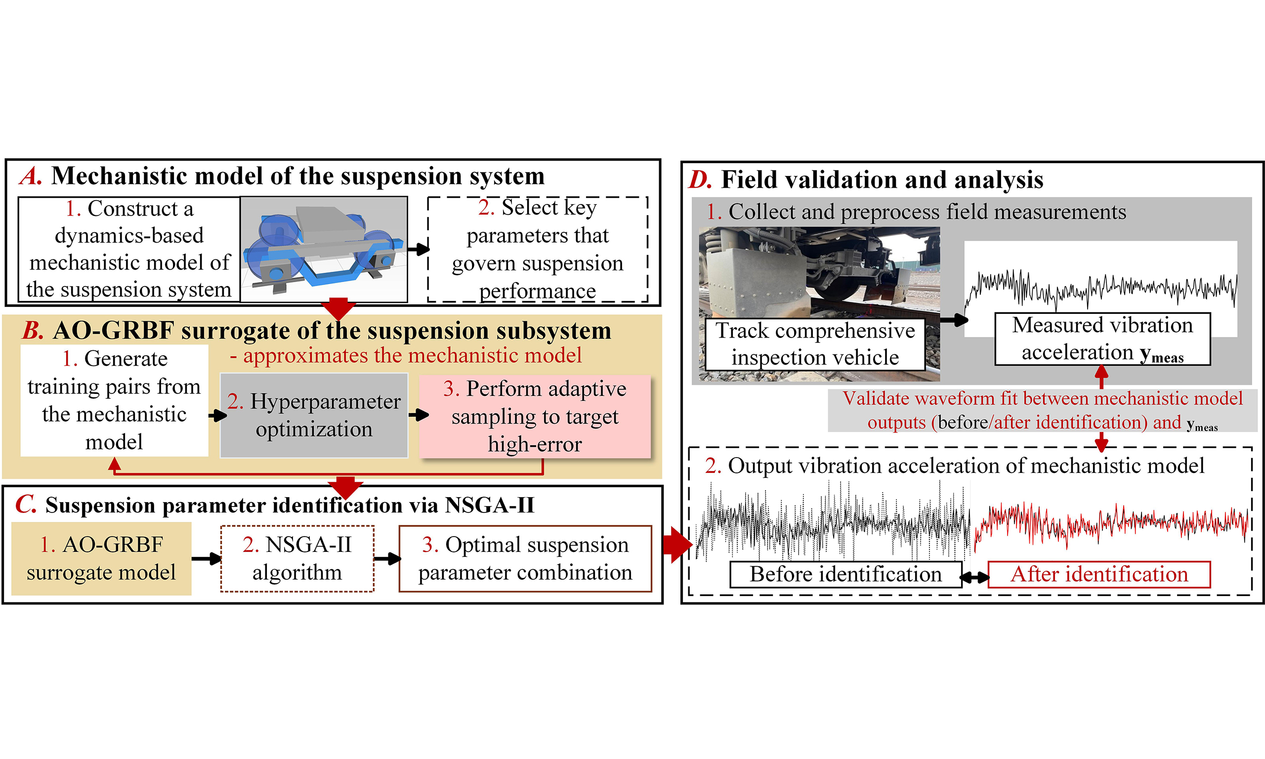
The framework of the proposed method is shown in Figure 1. In Module A, a train dynamics model is constructed on the SIMPACK platform to generate simulated vibration data under diverse suspension parameter configurations. To enhance the spatial representativeness of the simulation dataset, an adaptive sampling strategy is employed, and the resulting dataset is used to establish an AO-GRBF surrogate to replace the original dynamics model. Subsequently, in Module B, NSGA-II is applied to optimize the AO-GRBF parameters, minimizing the discrepancy between model predictions and measured vibration data to determine the suspension parameter combination that reflects the actual system behavior.
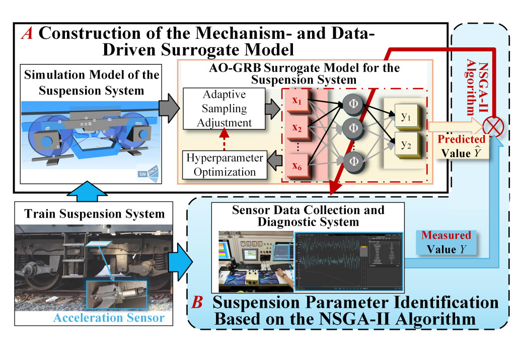
Figure 1. Overall framework diagram (photographs by the authors). AO-GRBF: Adaptively optimized Gaussian radial basis function; NSGA-II: nondominated sorting genetic algorithm II.
3.1. Construction of the mechanism- and data-driven AO-GRBF surrogate model
To expedite suspension parameter identification, a data-driven AO-GRBF surrogate model for the suspension system is constructed in this section. The approach comprises: (1) mechanism-based training dataset generation via MBD modeling; (2) construction of the data-driven AO-GRBF model with adaptive optimization techniques; and (3) model performance validation.
3.1.1. MBD model of rail transit vehicle
Scenarios involving suspension parameter degradation cannot be safely reproduced through real-vehicle testing and pose substantial safety risks. To enable simulation and obtain vehicle vibration responses under different suspension parameter configurations, a train multibody dynamics model is constructed on the SIMPACK platform. The model incorporates critical nonlinear characteristics, including axle-box suspension clearances and dry friction in friction wedges [24,25]. Additionally, the wheel-rail contact is represented using Hertzian theory combined with the FASTSIM algorithm [26,27].
The validated train multibody dynamics model [28,29] comprises both primary and secondary suspension systems (highlighted in red boxes in Figure 2), which are designed to control load bearing and ensure ride stability. Fourteen suspension parameters (
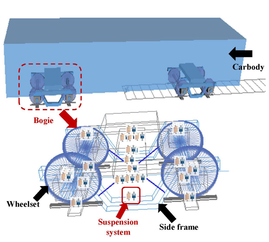
Figure 2. Dynamic modeling structure of the train and its suspension system.
VIP values of all suspension parameters
| Symbol | Parameter name | Unit | Original value | Value range | VIP( | VIP( |
| Bold values indicate | ||||||
| Lateral stiffness of the primary steel spring | MN/m | 0.98 | 0.10–9.8 | 0.0252 | 0.15303 | |
| Longitudinal stiffness of the primary steel spring | MN/m | 0.98 | 0.10–9.8 | 0.55299 | 0.34093 | |
| Vertical stiffness of the primary steel spring | MN/m | 4.52 | 0.45–45.2 | 1.5818 | 3.17028 | |
| Lateral stiffness of the primary axle box arm joint | MN/m | 13.70 | 1.37–137.0 | 0.26975 | 0.03386 | |
| Longitudinal stiffness of the primary axle box arm joint | MN/m | 5.52 | 0.55–55.2 | 2.94629 | 0.52944 | |
| Vertical stiffness of the primary axle box arm joint | MN/m | 5.52 | 0.55–55.2 | 0.02464 | 0.20156 | |
| Stiffness of the primary vertical damper joint | MN/m | 0.62 | 0.06–6.2 | |||
| Damping of the primary vertical damper | MN/m | 0.01 | 0.00–0.1 | 0.10559 | 0.35821 | |
| Lateral stiffness of the secondary air spring | MN/m | 0.17 | 0.02–1.7 | 0.21934 | ||
| Longitudinal stiffness of the secondary air spring | MN/m | 0.17 | 0.02–1.7 | 0.45688 | 0.15309 | |
| Vertical stiffness of the secondary air spring | MN/m | 12.32 | 1.23–123.2 | 0.18619 | 1.62243 | |
| Stiffness of the secondary lateral damper joint | MN/m | 17.20 | 1.72–172.0 | 0.00487 | 0.08812 | |
| Stiffness of the secondary antihunting damper joint | MN/m | 8.82 | 0.88–88.2 | 1.13243 | 0.24706 | |
| Longitudinal stiffness of the secondary traction rod | MN/m | 7.88 | 0.79–78.8 | 0.28475 | 0.30521 | |
The variable importance in projection (VIP) method is applied to identify critical suspension parameters based on their contributions to carbody vibration acceleration through partial least squares (PLS) regression analysis[30]. The VIP value (
where
To ensure accurate VIP calculation, parameter ranges are determined based on the initial suspension parameters and historical data from heavy-haul railways, as summarized in Table 1. Parameter sampling is performed using the multiobjective Latin hypercube design (MOLHD) method to reduce the risk of local optima while respecting computational resource constraints. This method employs an improved iterative local search (ILS) algorithm to optimize both sample uniformity and orthogonality. Several optimization criteria are combined to guarantee the representativeness of the samples[30]. In total, 200 sets of suspension parameter values are generated through MOLHD, and the train multibody dynamics model is subsequently evaluated on these samples to obtain the root-mean-square values of lateral (
Based on the VIP results in Table 1, six parameters are retained for surrogate-model-based identification to capture their influence on both lateral and vertical vibration responses. Four parameters with VIP values exceeding 1.0 are selected: vertical stiffness of the primary steel spring (
The six selected parameters are renumbered as
Selected key suspension parameter ranges for surrogate model training
| Symbol | Parameter name | Unit | Nominal value | Sampling range | Original symbol |
| Vertical stiffness of the primary steel spring | MN/m | 4.52 | 2.26–9.04 | ||
| Longitudinal stiffness of the primary axle-box arm joint | MN/m | 5.52 | 2.76–11.04 | ||
| Stiffness of the primary vertical damper joint | MN/m | 0.62 | 0.31–1.24 | ||
| Lateral stiffness of the secondary air spring | MN/m | 0.17 | 0.085–0.34 | ||
| Vertical stiffness of the secondary air spring | MN/m | 12.32 | 6.16–24.64 | ||
| Stiffness of the secondary antihunting damper joint | MN/m | 8.82 | 4.41–17.64 |
3.1.2. Surrogate modeling via AO-GRBF
To accelerate the suspension parameter identification process, an AO-GRBF data-driven surrogate is constructed to approximate the nonlinear mapping from suspension parameters to vibration acceleration responses. Training and validation datasets are generated with the established MBD model to provide the data required for surrogate construction:
where
The surrogate model structure is represented as[31]:
where
where
The hyperparameters
where
To improve local fidelity, adaptive sampling is performed based on the residual error metric:
where
where
The iterative procedure is terminated when the relative change in hyperparameters satisfies:
where
3.1.3. Validation of the AO-GRBF surrogate model
For comparability, the proposed AO-GRBF Surrogate Model is evaluated against five representative surrogate models: GRBF [10], radial basis function neural network (RBFNN) [35], radial basis function high-dimensional model representation (RBF-HDMR) [36], long short-term memory (LSTM) networks [37], and Transformer networks [38]. RBF-HDMR integrates the efficiency of RBF with dimensionality reduction to address complex multiphysics problems through hierarchical decomposition. LSTM and Transformer models are adopted as representative deep learning approaches for sequential data prediction. All models are trained and validated on datasets generated by the SIMPACK-based multibody simulation model.
Prediction accuracy is evaluated using the coefficient of determination (
where
The AO-GRBF model achieves the highest
| Vibration direction | GRBF[10] | RBFNN[35] | RBF-HDMR[36] | LSTM[37] | Transformer[38] | Proposed AO-GRBF |
| Bold values denote the results of the proposed AO-GRBF method. GRBF: Gaussian radial basis function; RBFNN: radial basis function neural network; RBF-HDMR: radial basis function high-dimensional model representation; LSTM: long short-term memory; AO-GRBF: adaptively optimized Gaussian radial basis function; Lateral: lateral vibration acceleration; Vertical: vertical vibration acceleration. | ||||||
| Lateral | 0.7024 | 0.7307 | 0.7847 | 0.7196 | 0.7348 | 0.8240 |
| Vertical | 0.8455 | 0.8997 | 0.9013 | 0.8847 | 0.9143 | 0.9386 |
The improvements are primarily attributed to NSGA-II-based hyperparameter optimization and error-guided adaptive sampling, which are used jointly to improve local accuracy and global robustness. By contrast, traditional methods present clear limitations. For RBFNN, center selection is driven by clustering algorithms, which can preclude the identification of optimal configurations. For RBF-HDMR, decomposition errors may be introduced in high-dimensional cases. In addition, both methods adopt fixed sampling strategies without adaptive refinement, which restricts flexibility. Deep learning approaches, such as LSTM and Transformer, are theoretically capable of capturing sequential dependencies; however, their effectiveness is reduced under the current dataset conditions. With limited and relatively homogeneous samples, LSTM models are prone to overfitting, whereas Transformer models face similar generalization issues and require extensive regularization. In comparison, the proposed AO-GRBF method achieves improved generalization through the combined use of error-guided adaptive sampling and a regularized kernel formulation.
3.2. Suspension parameter optimization based on NSGA-II
Based on the constructed AO-GRBF surrogate model, a mapping is established from the suspension parameters
The multiobjective optimization problem is formulated as:
where
The correlation coefficients and mean squared errors are computed as:
where
Based on the optimization objectives defined above, the NSGA-II algorithm performs parameter identification through the following steps:
(1) Population Initialization: An initial population of size
where
(2) Evolutionary Operations: For each generation
where
where
The parent and offspring populations are merged to form
where
(3) Termination: The algorithm terminates upon convergence, yielding the final Pareto-optimal parameter set:
The integration of AO-GRBF and NSGA-II forms a closed-loop identification process, as illustrated in Figure 3. At each iteration, deviations between the predicted
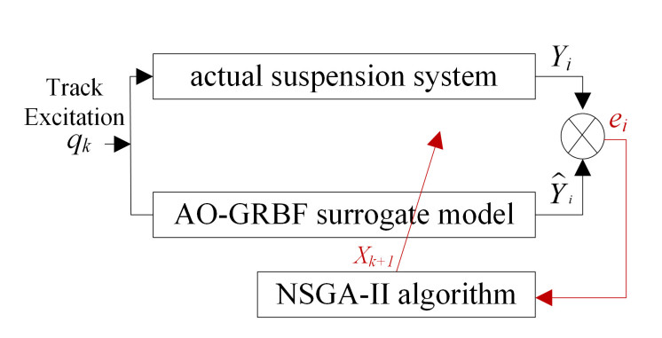
Figure 3. Closed-loop diagram integrating the AO-GRBF surrogate model and NSGA-II for parameter identification. AO-GRBF: Adaptively optimized Gaussian radial basis function; NSGA-II: nondominated sorting genetic algorithm II.
4. RESULTS
4.1. On-site data collection
The experimental dataset was collected along a heavy-haul railway line in China. Two categories of field measurements were obtained: (1) track-geometry irregularities (vertical profile, alignment, cross-level, superelevation, and gauge); and (2) carbody vibration accelerations. To ensure sufficient diversity in operating conditions for model training and evaluation, the dataset comprises multiple track segments that together cover small-radius curves, tangent sections, ascending grades, and descending grades.
The track irregularity data were recorded in real time using a track inspection system equipped with inertial navigation and vibration compensation modules, as shown in Figure 4. These data were subsequently used to construct a simulation environment that replicates actual operating conditions. In addition, carbody vibration accelerations were measured by accelerometers installed near the rear wheelset of the bogie, and all acceleration signals were sampled at a frequency of 100 Hz.
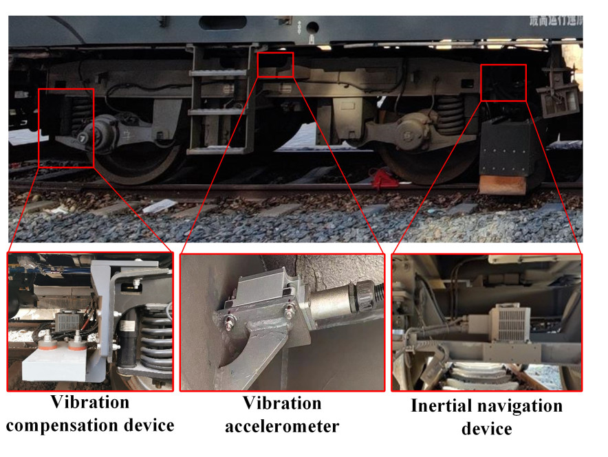
Figure 4. Track inspection system adopted for field measurements (photographs by the authors).
4.2. Result analysis
To evaluate the effectiveness of the proposed AO-GRBF-based identification framework, comparative experiments were conducted against the traditional G-RBF method, as well as recent approaches based on RBFNN and RBF-HDMR [10,35,36], and deep learning baselines including LSTM and Transformer networks [37,38]. All methods were executed on the same dataset generated by the SIMPACK model and under identical NSGA-II configurations to ensure a fair comparison.
The identified suspension parameter sets are summarized in Table 4, and the corresponding objective values predicted by the surrogates are provided in Table 5. Because some surrogates exhibit limited fitting accuracy and a propensity for local optima, the predicted results may deviate from the true system behavior. To validate the identification results, the optimal parameter sets in Table 4 were applied to a high-fidelity mechanistic train model implemented in SIMPACK. Furthermore, a 200 m operating subsegment from the field runs was selected to provide a common test condition. Simulations under this condition were conducted to generate vibration responses, enabling waveform-level and metric-level comparisons across methods.
Identified suspension parameter combinations by various methods
| Method | ||||||
| Bold values denote the identified parameter combination obtained by the proposed method. GRBF: Gaussian radial basis function; RBFNN: radial basis function neural network; RBF-HDMR: radial basis function-high-dimensional model representation; LSTM: long short-term memory; | ||||||
| GRBF[10] | 2.519797 | 5.025912 | 0.412473 | 0.192750 | 6.717632 | 14.674392 |
| RBFNN[35] | 2.406953 | 4.834850 | 0.456229 | 0.291226 | 6.498389 | 13.916075 |
| RBF-HDMR[36] | 3.836718 | 10.106013 | 0.917215 | 0.151945 | 7.707624 | 4.724100 |
| LSTM[37] | 2.986700 | 4.034600 | 0.769170 | 0.167720 | 13.162000 | 4.759400 |
| Transformer[38] | 2.403600 | 2.992900 | 0.972300 | 0.094003 | 13.129000 | 6.867100 |
| Proposed method | 2.451836 | 4.142077 | 0.777890 | 0.273584 | 17.414320 | 6.739952 |
Predicted objective function values of surrogate models under identified parameters
| Method | | | | |
| Bold values denote the predicted objective function values obtained by the proposed method. GRBF: Gaussian radial basis function; RBFNN: radial basis function neural network; RBF-HDMR: radial basis function-high-dimensional model representation; LSTM: long short-term memory; | ||||
| GRBF[10] | 0.6350 | 0.8567 | 0.00082 | 0.00194 |
| RBFNN[35] | 0.9870 | 0.6848 | 0.00000 | 0.00166 |
| RBF-HDMR[36] | 0.9938 | 0.8232 | 0.00046 | 0.00073 |
| LSTM[37] | 0.9600 | 0.7141 | 0.00020 | 0.00454 |
| Transformer[38] | 0.9044 | 0.9113 | 0.00025 | 0.00058 |
| Proposed method | 0.9256 | 0.9738 | 0.00045 | 0.00056 |
The lateral and vertical vibration accelerations before and after parameter identification are compared in Figures 5 and 6. The predicted responses (blue) show varying degrees of agreement with the measured data (black), compared with the unidentified baseline (black dashed line), thereby confirming the effectiveness of surrogate-assisted parameter identification. As shown in Figures 5A and 6A, both the AO-GRBF method (red) and G-RBF (blue) improve waveform alignment, with AO-GRBF achieving closer amplitude agreement and more accurate phase matching.
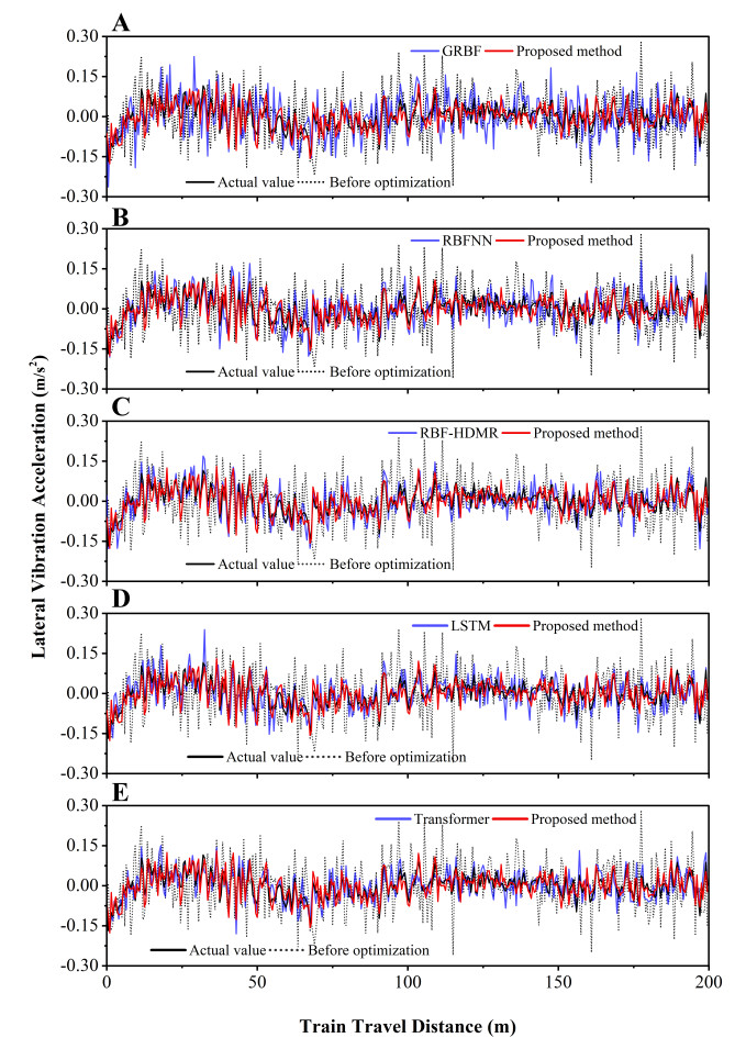
Figure 5. Comparison of lateral vibration acceleration before and after parameter identification by various methods. (A) Comparison with GRBF; (B) Comparison with RBFNN; (C) Comparison with RBF-HDMR; (D) Comparison with LSTM; (E) Comparison with Transformer. All subfigures show the measured data (black) and the unidentified baseline (black dashed) as references. The proposed method (red) and other approaches exhibit different levels of consistency with the experimental observations. GRBF: Gaussian radial basis function; RBFNN: radial basis function neural network; RBF-HDMR: radial basis function high-dimensional model representation; LSTM: long short-term memory.
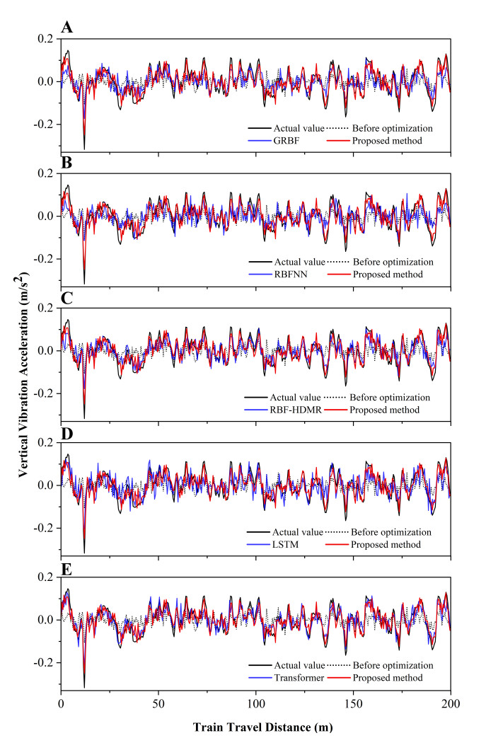
Figure 6. Comparison of vertical vibration acceleration before and after parameter identification by various methods. (A) Comparison with GRBF; (B) Comparison with RBFNN; (C) Comparison with RBF-HDMR; (D) Comparison with LSTM; (E) Comparison with Transformer. All subfigures show the measured data (black) and the unidentified baseline (black dashed) as references. The proposed method (red) and other approaches show different levels of consistency with experimental observations. GRBF: Gaussian radial basis function; RBFNN: radial basis function neural network; RBF-HDMR: radial basis function high-dimensional model representation; LSTM: long short-term memory.
Further comparisons with RBFNN, RBF-HDMR, LSTM, and Transformer methods are presented in Figure 5B-E and 6B-E. Among these methods, RBF-HDMR (blue) generates vibration responses that closely approximate the measured data (black), as illustrated in Figures 5C and 6C. Transformer networks (blue) also provide improved overall waveform alignment, as shown in Figures 5E and 6E. Consequently, the responses produced by RBF-HDMR (blue), Transformer (blue), and the proposed AO-GRBF method (red) are closely aligned with the measured data, and visual inspection alone does not clearly indicate which method achieves the best identification performance.
To quantitatively assess performance, the Pearson correlation coefficients (
Actual objective function values under each parameter identification method
| Method | | | | |
| Bold values denote the actual objective function values obtained by the proposed method. GRBF: Gaussian radial basis function; RBFNN: radial basis function neural network; RBF-HDMR: radial basis function-high-dimensional model representation; LSTM: long short-term memory; | ||||
| No identification | 0.29741 | 0.49937 | 0.00811 | 0.00314 |
| GRBF[10] | 0.47318 | 0.77027 | 0.00405 | 0.00180 |
| RBFNN[35] | 0.79343 | 0.65471 | 0.00141 | 0.00236 |
| RBF-HDMR[36] | 0.81877 | 0.84978 | 0.00119 | 0.00127 |
| LSTM[37] | 0.73891 | 0.71823 | 0.00155 | 0.00201 |
| Transformer[38] | 0.78354 | 0.88790 | 0.00116 | 0.00092 |
| Proposed method | 0.84415 | 0.91317 | 0.00073 | 0.00073 |
Relative to RBF-HDMR, which adopts a dimensional decomposition strategy, the proposed method achieves additional improvements of 3.10% in
4.3. Computational efficiency analysis
To evaluate real-time feasibility for practical suspension parameter identification, a computational efficiency analysis was conducted. Experiments were performed on a workstation equipped with an Intel Core i9-14900KF CPU, 64GB RAM, and an NVIDIA GeForce RTX 4060 Ti. A high-fidelity mechanistic train model was constructed on the SIMPACK 2021x/SIMPACK Post 2021x platform. Mechanism-based identification with NSGA-II was realized by coupling MATLAB R2021a with SIMPACK 2021x, whereas surrogate construction (GRBF, RBFNN, RBF-HDMR, LSTM, Transformer, AO-GRBF) and surrogate-based identification with NSGA-II were implemented in MATLAB R2021a.
For a fair comparison, the total runtime is defined separately for the two categories of methods. For the high-fidelity mechanistic approach, total runtime denotes the elapsed time of a complete identification run, in which NSGA-II, implemented in MATLAB R2021a, directly executes the SIMPACK-based train model. For surrogate-based approaches, total runtime equals the sum of surrogate construction time in MATLAB R2021a (including training and tuning) and the subsequent NSGA-II search performed on the surrogate.
Parameter identification with the proposed AO-GRBF method is completed in 1.25 min [Table 7], yielding a speedup of approximately 3, 010
Computational time comparison of different methods
| Method | Total runtime (min) |
| Bold values denote the total runtime obtained by the proposed method. MBD: Multibody dynamics; GRBF: Gaussian radial basis function; RBFNN: radial basis function neural network; RBF-HDMR: radial basis function-high-dimensional model representation; LSTM: long short-term memory. | |
| High-fidelity MBD simulation | 3, 762 |
| GRBF[10] | 0.30 |
| RBFNN[35] | 0.39 |
| RBF-HDMR[36] | 1.01 |
| LSTM[37] | 4.16 |
| Transformer[38] | 4.21 |
| Proposed method | 1.25 |
Although classical surrogates (GRBF, RBFNN) complete the process more quickly due to their simpler structures, their predictive accuracy is lower [Table 6]. Deep learning-based surrogates (LSTM, Transformer) require more than 4 min, which is about 3.3 times the runtime of the proposed method. Overall, the AO-GRBF approach achieves a favorable balance between computational efficiency and estimation accuracy, enabling time-critical suspension parameter identification and supporting rapid detection of stiffness and damping changes for proactive safety management.
4.4. Method stability analysis
To evaluate the robustness of the proposed AO-GRBF framework under repeated surrogate retraining, a stability analysis was conducted across 20 independent trials. In each trial, the training and validation datasets
The distributions of the identified suspension parameters are shown in Figure 7. All parameters exhibit compact clustering, and the coefficients of variation are below 9%, indicating consistent identification performance across trials. In particular,
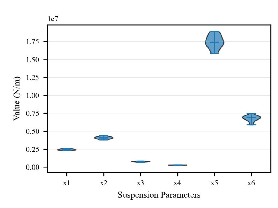
Figure 7. Distributions of the identified suspension parameters
To quantify stability, performance deviations were computed relative to the baseline results in Section 4.2. For each trial, the identified parameters were evaluated using the high-fidelity SIMPACK model to obtain the correlation coefficients
The relationship between performance accuracy and the magnitude of parameter deviation is illustrated in Figure 8. For vertical vibration correlation,
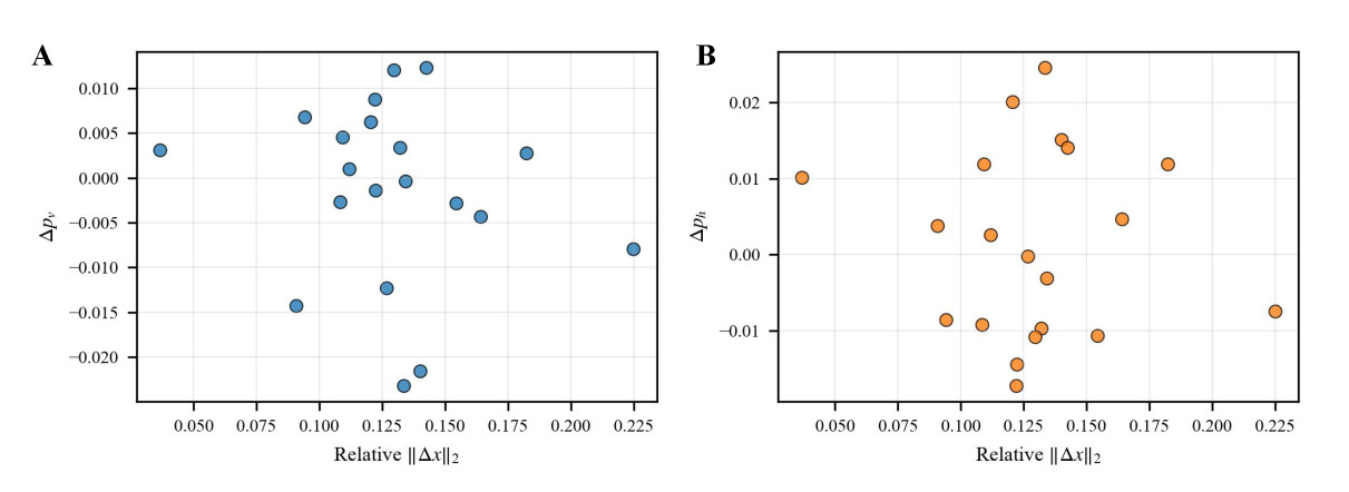
Figure 8. Performance deviations versus relative parameter deviation magnitude. (A) Vertical correlation deviation
The trial-wise performance variations are depicted in Figure 9. Both
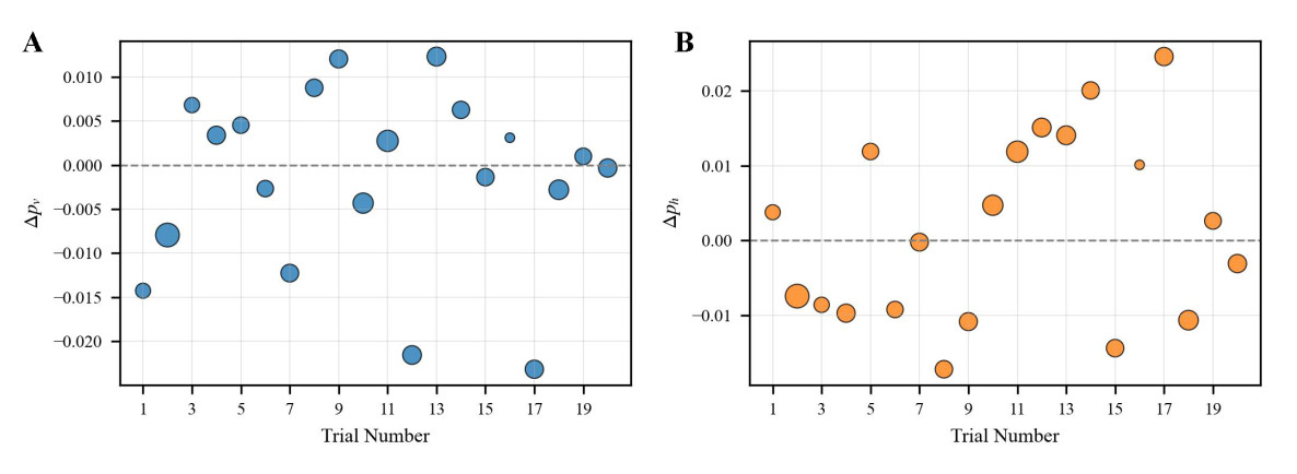
Figure 9. Trial-wise performance deviations across 20 independent trials. (A) Vertical correlation deviation
To more comprehensively assess model robustness, an error space analysis is conducted to quantify absolute accuracy relative to the identification objective. Figure 10 reports trial-wise deviations of the mean squared acceleration error,
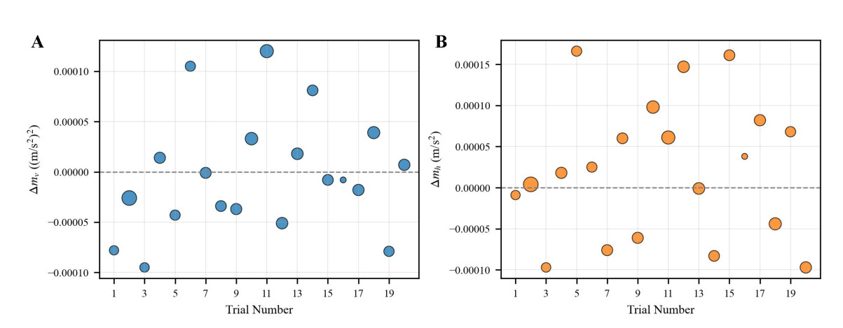
Figure 10. Trial-wise deviations of error-type metrics relative to the baseline. (A) Deviation in the mean squared error of vertical acceleration (
The stability analysis indicates that consistent identification performance is achieved across independent trials, with deviations remaining within acceptable engineering tolerances. This robustness is attributed to the combined use of error-guided adaptive sampling and NSGA-II optimization, which ensures reliable convergence despite dataset variability typical of practical applications.
5. DISCUSSION
An AO-GRBF surrogate model coupled with NSGA-II was introduced to identify suspension parameters. Adaptive sampling and multiobjective hyperparameter optimization were employed to improve robustness. The results indicate that the framework provides a practical surrogate-assisted optimization strategy for nonlinear and time-varying vehicle dynamics, while maintaining accuracy and computational efficiency. Notably, suspension parameter identification typically operates in small-data regimes (simulation-supported samples with modest field measurements), unlike vision tasks such as image recognition or generation that rely on very large datasets. Accordingly, the conclusions are framed within this small-data setting rather than for large-scale training scenarios. The comparative results against deep learning baselines should therefore be interpreted within this small-data context.
Several limitations should be acknowledged. Field-measured vibration and track irregularity data are often affected by measurement errors, missing data, and fluctuating operating conditions. These factors may undermine the stability of parameter identification. Similar issues have been reported in data-driven studies, where data uncertainty was found to reduce the reliability of surrogate modeling [39,40].
To mitigate the impact of measurement inaccuracies and data loss, future research is encouraged to incorporate uncertainty quantification and data reconciliation methods. Another direction is to integrate online or incremental learning strategies to enable continuous refinement of parameter estimates as new data become available [41]. Beyond suspension systems, the framework may be extended to related fields in intelligent transportation and robotics, including wheel-rail contact modeling and mechatronic subsystems that require efficient surrogate-assisted parameter identification. Furthermore, reliable sensing and distributed computing resources are expected to support these applications.
6. CONCLUSIONS
This paper presented a suspension parameter identification method that integrates an AO-GRBF surrogate model with the NSGA-II algorithm. The approach was designed to approximate nonlinear dynamics and to identify parameters consistent with measured responses.
First, an error-aware sampling strategy was employed to emphasize regions with higher residuals, and a multiobjective tuning procedure was used to adjust kernel and regularization parameters to balance generalization. Next, the surrogate model was coupled with multiobjective optimization to generate parameter sets that align with field vibration data. Finally, validation using on-site measurements of vibration and track irregularities confirmed higher correlation and lower error than other surrogate-based approaches, with improvements observed in both lateral and vertical indicators.
In summary, this study provides a data-driven and mechanism-informed framework for suspension identification. Supported by field experiments, the method demonstrates advantages over existing techniques and shows potential for extension to intelligent transportation and robotic systems where efficient parameter estimation is required.
DECLARATIONS
Authors’ contributions
Experimental analysis and manuscript writing: Jiang, S.
Overall study design, conceptual framework development, and methodological guidance: Liu, J.
Technical support: Yang, S. X.
Availability of data and materials
Restrictions apply to the availability of these data. Field measurements were obtained from a heavy-haul railway line using proprietary inspection equipment under a collaboration agreement with a commercial railway operator (third party); therefore, public release is not permitted. Data may be made available from the corresponding author upon reasonable request and with prior written permission from the data owner, subject to confidentiality and data use agreements.
AI and AI-assisted tools statement
Not applicable.
Financial support and sponsorship
This work was supported in part by the National Key R & D Program of China (Grant No. 2021YFF0501101), the National Natural Science Foundation of China (Grant No. 52272347), the Natural Science Foundation of Hunan Province (Grant No. 2024JJ7132), and the Scientific Research Project of Hunan Provincial Department of Education (Grant No. 22A0391).
Conflicts of interest
Yang, S. X. is the Editor-in-Chief of the journal Intelligence & Robotics. He is not involved in any steps of editorial processing, notably including reviewers’ selection, manuscript handling and decision making. The other authors declare that there are no conflicts of interest.
Ethical approval and consent to participate
Not applicable.
Consent for publication
Not applicable.
Copyright
© The Author(s) 2026.
REFERENCES
1. Na, J.; Huang, Y.; Wu, X.; Liu, Y. J.; Li, Y.; Li, G. Active suspension control of quarter-car system with experimental validation. IEEE. Trans. Syst. Man. Cybern. Syst. 2022, 52, 4714-26.
2. Bai, R.; Wang, H. B. Robust optimal control for the vehicle suspension system with uncertainties. IEEE. Trans. Cybern. 2022, 52, 9263-73.
3. Pan, Y.; Sun, Y.; Li, Z.; Gardoni, P. Machine learning approaches to estimate suspension parameters for performance degradation assessment using accurate dynamic simulations. Reliab. Eng. Syst. Saf. 2023, 230, 108950.
4. Jiang, X.; Xu, X.; Shi, T.; Atindana, V. A. Nonlinear characteristic analysis of gas-interconnected quasi-zero stiffness pneumatic suspension system: a theoretical and experimental study. Chin. J. Mech. Eng. 2024, 37, 58.
5. Liu, J.; Du, D.; He, J.; Zhang, C. Prediction of remaining useful life of railway tracks based on DMGDCC-GRU hybrid model and transfer learning. IEEE. Trans. Veh. Technol. 2024, 73, 7561-75.
6. Zhang, Y. W.; Zhao, Y.; Zhang, Y. H.; Lin, J. H.; He, X. W. Riding comfort optimization of railway trains based on pseudo-excitation method and symplectic method. J. Sound. Vib. 2013, 332, 5255-70.
7. Bruni, S.; Meijaard, J. P.; Rill, G.; Schwab, A. L. State-of-the-art and challenges of railway and road vehicle dynamics with multibody dynamics approaches. Multibody. Syst. Dyn. 2020, 49, 1-32.
8. Kraft, S.; Puel, G.; Aubry, D.; Fünfśchilling, C. Parameter identification of multi-body railway vehicle models - application of the adjoint state approach. Mech. Syst. Signal. Process. 2016, 80, 517-32.
9. Yang, Y.; Zeng, W.; Qiu, W. S.; Wang, T. Optimization of the suspension parameters of a rail vehicle based on a virtual prototype Kriging surrogate model. Proc. Inst. Mech. Eng. 2016, 230, 1890-8.
10. Chen, G.; Zhang, K.; Xue, X.; et al. A radial basis function surrogate model assisted evolutionary algorithm for high-dimensional expensive optimization problems. Appl. Soft. Comput. 2022, 116, 108353.
11. Ni, P.; Li, J.; Hao, H.; Zhou, H. Reliability based design optimization of bridges considering bridge-vehicle interaction by Kriging surrogate model. Eng. Struct. 2021, 246, 112989.
12. Wei, F. F.; Chen, W. N.; Mao, W.; Hu, X. M.; Zhang, J. An efficient two-stage surrogate-assisted differential evolution for expensive inequality constrained optimization. IEEE. Trans. Syst. Man. Cybern. Syst. 2023, 53, 7769-82.
13. Chen, Q.; Zhang, H.; Zhou, H.; Sun, J.; Tian, Y. Adaptive design of experiments for fault injection testing of highly automated vehicles. IEEE. Intell. Transp. Syst. Mag. 2024, 16, 35-52.
14. Zhang, L.; Li, T.; Zhang, J.; Piao, R. Optimization on the crosswind stability of trains using neural network surrogate model. Chin. J. Mech. Eng. 2021, 34, 86.
15. Zhang, C.; Wang, Y.; He, J. Suspension parameter estimation method for heavy-duty freight trains based on deep learning. Big. Data. Cogn. Comput. 2024, 8, 181.
16. Jiang, R.; Jin, Z.; Liu, D.; Wang, D. Multi-objective lightweight optimization of parameterized suspension components based on NSGA-II algorithm coupling with surrogate model. Machines 2021, 9, 107.
17. Gu, J.; Hua, W.; Yu, W.; Zhang, Z.; Zhang, H. Surrogate model-based multiobjective optimization of high-speed permanent magnet synchronous machine: construction and comparison. IEEE. Trans. Transp. Electr. 2023, 9, 678-88.
18. Liu, C.; Wan, Z.; Liu, Y.; Li, X.; Liu, D. Trust-region based adaptive radial basis function algorithm for global optimization of expensive constrained black-box problems. Appl. Soft. Comput. 2021, 105, 107233.
19. Ye, N.; Long, T.; Shi, R.; Wu, Y. Radial basis function-assisted adaptive differential evolution using cooperative dual-phase sampling for high-dimensional expensive optimization problems. Struct. Multidiscip. Optim. 2022, 65, 241.
20. Yao, Y.; Chen, X.; Li, H.; Li, G. Suspension parameters design for robust and adaptive lateral stability of high-speed train. Veh. Syst. Dyn. 2023, 61, 943-67.
21. Tsattalios, S.; Tsoukalas, I.; Dimas, P.; Kossieris, P.; Efstratiadis, A.; Makropoulos, C. Advancing surrogate-based optimization of time-expensive environmental problems through adaptive multi-model search. Environ. Model. Softw. 2023, 162, 105639.
22. Hua, C.; Jiang, C.; Niu, R.; et al. Double neural networks enhanced global mobility prediction model for unmanned ground vehicles in off-road environments. IEEE. Trans. Veh. Technol. 2024, 73, 7547-60.
23. Tong, H.; Huang, C.; Minku, L. L.; Yao, X. Surrogate models in evolutionary single-objective optimization: a new taxonomy and experimental study. Inform. Sci. 2021, 562, 414-37.
24. Flores, P.; Ambrósio, J.; Lankarani, H. M. Contact-impact events with friction in multibody dynamics: back to basics. Mech. Mach. Theory. 2023, 184, 105305.
25. Millan, P.; Pagaimo, J.; Magalhães, H.; Ambrósio, J. Clearance joints and friction models for the modelling of friction damped railway freight vehicles. Multibody. Syst. Dyn. 2023, 58, 21-45.
26. Zhou, Y.; Mei, T. X.; Freear, S. Real-time modeling of wheel-rail contact laws with system-on-chip. IEEE. Trans. Parallel. Distrib. Syst. 2010, 21, 672-84.
27. Liu, B.; Bruni, S. Comparison of wheel-rail contact models in the context of multibody system simulation: Hertzian versus non-Hertzian. Veh. Syst. Dyn. 2022, 60, 1076-96.
28. Wu, H.; Zeng, X. H.; Lai, J.; Yu, Y. Nonlinear hunting stability of high-speed railway vehicle on a curved track under steady aerodynamic load. Veh. Syst. Dyn. 2020, 58, 175-97.
29. Sun, J.; Meli, E.; Song, X.; Chi, M.; Jiao, W.; Jiang, Y. A novel measuring system for high-speed railway vehicles hunting monitoring able to predict wheelset motion and wheel/rail contact characteristics. Veh. Syst. Dyn. 2023, 61, 1621-43.
30. Chen, X.; Huang, J.; Yi, M. Cost estimation for general aviation aircrafts using regression models and variable importance in projection analysis. J. Clean. Prod. 2020, 256, 120648.
31. Broomhead, D. S.; Lowe, D. Radial basis functions, multi-variable functional interpolation and adaptive networks. 1988. https://apps.dtic.mil/sti/html/tr/ADA196234/. (accessed 2026-03-20).
32. Zheng, W.; Doerr, B. Approximation guarantees for the non-dominated sorting genetic algorithm II (NSGA-II). IEEE. Trans. Evol. Comput. 2024, 891-905.
33. Zhang, D.; Li, C.; Luo, S.; et al. Multi-objective control of residential HVAC loads for balancing the user's comfort with the frequency regulation performance. IEEE. Trans. Smart. Grid. 2022, 13, 3546-57.
34. Ma, Y.; Xiao, Y.; Wang, J.; Zhou, L. Multicriteria optimal Latin hypercube design-based surrogate-assisted design optimization for a permanent-magnet vernier machine. IEEE. Trans. Magn. 2021, 58, 1-5.
35. Yuan, Z.; Kong, L.; Gao, D.; et al. Multi-objective approach to optimize cure process for thick composite based on multi-field coupled model with radial basis function surrogate model. Compos. Commun. 2021, 24, 100671.
36. Li, G.; Yao, Y.; Shen, L.; Deng, X.; Zhong, W. Influence of yaw damper layouts on locomotive lateral dynamics performance: Pareto optimization and parameter analysis. J. Zhejiang. Univ. Sci. A. 2023, 24, 450-64.
37. Zhao, Z.; Chen, W.; Wu, X.; Chen, P. C. Y.; Liu, J. LSTM network: a deep learning approach for short-term traffic forecast. IET. Intell. Trans. Syst. 2017, 11, 68-75.
38. Yao, H. Y.; Wan, W. G.; Li, X. End-to-end pedestrian trajectory forecasting with transformer network. ISPRS. Int. J. Geo. Inf. 2022, 11, 44.
39. Suawa, P.F.; Halbinger, A.; Jongmanns, M.; Reichenbach, M. Noise-robust machine learning models for predictive maintenance applications. IEEE. Sens. J. 2023, 23, 15081-92.
40. Lecuyer, M.; Atlidakis, V.; Geambasu, R.; Hsu, D.; Jana, S. Certified robustness to adversarial examples with differential privacy. In 2019 IEEE Symposium on Security and Privacy (SP), San Francisco, USA, May 19-23, 2019; IEEE, 2019; pp. 656–72.
Cite This Article
How to Cite
Download Citation
Export Citation File:
Type of Import
Tips on Downloading Citation
Citation Manager File Format
Type of Import
Direct Import: When the Direct Import option is selected (the default state), a dialogue box will give you the option to Save or Open the downloaded citation data. Choosing Open will either launch your citation manager or give you a choice of applications with which to use the metadata. The Save option saves the file locally for later use.
Indirect Import: When the Indirect Import option is selected, the metadata is displayed and may be copied and pasted as needed.
About This Article
Copyright

Data & Comments
Data
0


Comments
Comments must be written in English. Spam, offensive content, impersonation, and private information will not be permitted. If any comment is reported and identified as inappropriate content by OAE staff, the comment will be removed without notice. If you have any queries or need any help, please contact us at [email protected].