Download PDF
Research Article  |  Open Access  |  26 Mar 2026

Neurodynamics- and observer-based distributed robust formation control for mobile robots

Views: 69 |  Downloads: 0 |  Cited:  0
Intell. Robot. 2026, 6(1), 148-62.
10.20517/ir.2026.08 |  © The Author(s) 2026.
Author Information
Article Notes
Cite This Article

Abstract

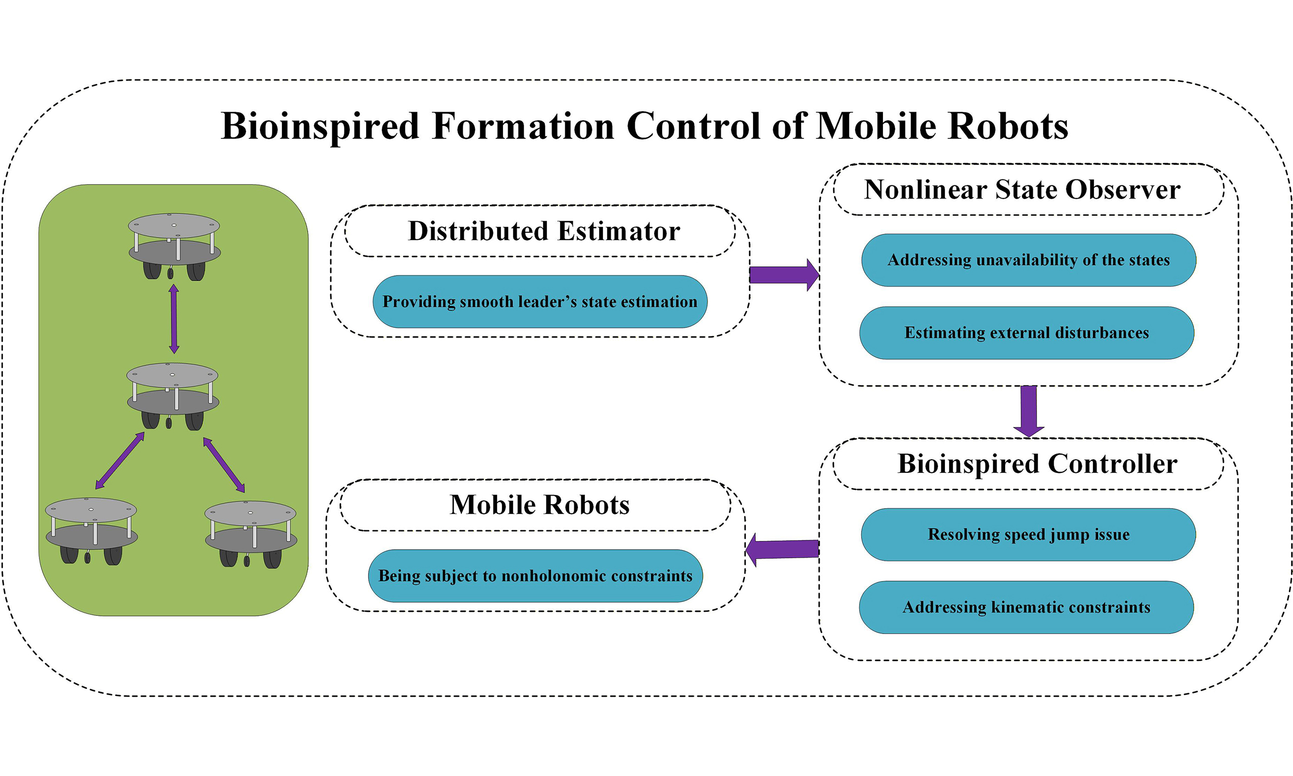
The formation control of multiple robot systems presents significant challenges due to practical constraints such as disturbances, speed discontinuities, velocity constraints, and incomplete state information. This paper introduces a novel biologically inspired control scheme that effectively addresses these challenges. First, utilizing the cascade design technique, a distributed estimator is presented to provide smooth estimates of the leader’s state without requiring derivative information. Subsequently, a nonlinear state estimator is proposed to provide accurate estimates of both states and disturbances. After that, a biologically inspired kinematic controller is developed that effectively resolves the speed surge and velocity constraint issues. Following the kinematic control design, a robust dynamic controller is developed based on the observed state to enhance robustness against disturbances. Finally, extensive simulation studies validate the effectiveness of the proposed approach and verify the theoretical results.

Keywords

Formation control, neural dynamics, mobile robot, distributed estimation

1. INTRODUCTION

Autonomous robotic platforms are increasingly valued in sectors such as emergency rescue missions, agriculture, and environmental monitoring [14]. Formation control has been a core research topic within multirobot collaboration and still attracts much research attention. The current formation techniques are classified mainly into the following categories: behavior-based approach [57], leader-follower based approach [810], and virtual structure approaches [1113]. Among these methods, the leader-follower approach has been widely adopted in industrial practice due to its architectural simplicity and ease of implementation [10,14,15]. This approach maintains a predefined formation by setting specific robots as the navigation reference, and the rest of the follower dynamically adjusts their relative positions to maintain the formation.

It is noticed that the robustness of the traditional centralized strategy decreases drastically when the number of following units increases, and failure of the leader node may trigger a system-level failure. Furthermore, the effectiveness of the system is strongly correlated with communication quality, and the surge of the network load is prone to lead to latency and deterioration of stability. To overcome these bottlenecks, modern research has increasingly adopted distributed control frameworks, which are developed based on local information exchange and awareness of neighboring states, thereby enhancing the system's fault tolerance and scalability [16,17]. There has been a significant amount of work that addresses the distributed formation approach of mobile robots [1822]. However, the formation performance heavily depends on the state estimation accuracy. In the work by Peng et al., an extended state observer along with a Kalman filter is developed to compensate for the disturbances and noises for mobile robots[23]. Another research proposed a fixed-time extended state observer that observes the total disturbances [24]. This research uses their respective approach to estimate the disturbances and the robot states. Furthermore, formation performance depends not only on the accuracy of the estimation techniques but also on the handling of practical constraints, such as velocity surge at the initial stage and velocity constraints, which occur in some of the existing work [25,26]. To better understand the velocity surge, it is described that when there is an initial error, the generated velocity is non-zero and therefore potentially generates an unreachable infinite torque command. Therefore, taking these critical challenges into the design of the formation control is rather important.

In this research, we address distributed leader-following in multi-mobile robot formation control and systematically solve three core challenges, namely unknown states, velocity jumps, and dynamic constraints. Firstly, to achieve consensus, a distributed observer is constructed to carry out the estimation of the leader's positional and velocity states through the local information interaction among the following nodes. Then, we construct a nonlinear estimation scheme to realize the robot states under uncertain external perturbations. After that, we introduce the adaptive response mechanism of biological neurons to construct a neurodynamic motion controller, which effectively resolves the steep changes in velocity commands observed in some existing works and ensures that these commands remain within preset thresholds. In addition, a dynamic controller is implemented that ensures the robust behavior of mobile robots in the presence of external perturbations. This hierarchical progressive control architecture is demonstrated through simulation verification.

The main contributions of this work can be summarized as follows:

● A nonlinear observer is designed to accurately estimate the unavailable robot states while maintaining robustness against external disturbances.

● A bioinspired distributed control strategy is developed to mitigate sudden surges in velocity commands caused by initial tracking errors and to enforce velocity constraints imposed by the robots' physical limits.

● The overall formation control framework is theoretically proved to be stable, ensuring robustness and convergence of the multiple mobile robot system under disturbances.

The rest of the paper is as follows: Section 2 provides the communication model and the dynamic equations of the individual mobile robot. Then, Section 3 derives the distributed estimation method, state observer, and controllers with proved stability. After that, multiple simulation studies have demonstrated that the proposed distributed formation framework yields apparent advantages over the conventional method in Section 4. Finally, the conclusion is provided to emphasize the contribution of this study and to list some potential future work that can be done.

2. PRELIMINARIES AND PROBLEM STATEMENT

2.1. Communication topology

In this study, the communication relationship of a multi-robot system is mathematically modeled using graph theory. It is defined as follows: the system contains $$ n $$ robots (nodes), and its communication network is given by an undirected graph $$ \mathcal{G}=\{\mathcal{V}, \mathcal{E} \:\mathcal{A}\} $$ with node set $$ \mathcal{V}=\{1, \:2, \:..., n\} $$ and each node represents a robot. The edge set $$ \mathcal{E} \subseteq \mathcal{V} \times \mathcal{V} $$, if the robots $$ i $$ and $$ j $$ can communicate, then there exists an edge $$ (i, j) \in \mathcal{E} $$. The adjacency matrix $$ \mathcal{A}=[a_{ij}]_{n\times n} $$ indicates access to information from $$ i $$ to $$ j $$. In addition, $$ a_{ii}=0 $$ in this study. Define the Laplacian matrix $$ L=[\mathcal{L}_{ij}]_{n\times n} $$ to describe the network connectivity, where $$ \mathcal{L}_{ii}=\begin{matrix} \sum_{j=1}^n a_{ij} \end{matrix} $$ and $$ \mathcal{L}_{ij}=-a_{ij}, \:i \ne j $$. It denotes the communication between $$ n $$ followers, and is assumed to be connected. The leader is indexed as 0 and define $$ a = {\rm{diag}}({a_{10}}, \:..., \:{a_{n0}}) \in {^{{\rm{n}} \times {\rm{n}}}} $$ to reflect the communication between the leader and the followers. For elements in $$ a $$, it is defined that $$ a_{i0}>0 $$ if the follower $$ i $$ can directly obtain the leader's states and 0 otherwise. The communication network is represented by matrix $$ H $$, which is defined as $$ H = L+a $$. We then obtain Lemma 1.

Lemma 1. Matrix $$ H $$ is positive definite if the leader is the neighbor of at least one follower and $$ \mathcal{G} $$ is connected.

2.2. Problem statement

In this study, the general structure of the mobile robot is shown in Figure 1. It is assumed that all robots share a similar structure, with the front wheel being passive and the two rear wheels being driven. There are a total of $$ n $$ robots and one (virtual) leader. The kinematics of the follower $$ i $$ are given as

$$ \left[ {\begin{array}{*{20}{c}} {{\dot x_i}}\\ {{\dot y_i}}\\ {{\dot \theta _i}} \end{array}} \right] = \left[ {\begin{array}{*{20}{c}} {\begin{array}{*{20}{c}} {\cos {\theta _i}}\\ {\sin {\theta _i}}\\ 0 \end{array}}&{\begin{array}{*{20}{c}} 0\\ 0\\ 1 \end{array}} \end{array}} \right]\left[ {\begin{array}{*{20}{c}} {{\upsilon _i}}\\ {{\omega _i}} \end{array}} \right] $$

Neurodynamics- and observer-based distributed robust formation control for mobile robots

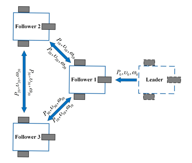
Figure 1. Mobile robot communication networks.

where $$ x_i $$ and $$ y_i $$ represent the position, and its angle of direction $$ \theta_i $$ is relative to the inertial frame; $$ \upsilon_i $$ and $$ \omega_i $$ represent the linear and angular velocities of the $$ i $$th mobile robot in body fixed frame, respectively.

Then, define leader's linear and angular velocities as $$ \upsilon_0 $$ and $$ \omega_0 $$, respectively, and their time derivatives are bounded. Then, there exist positive constants $$ \lambda_\upsilon $$ and $$ \lambda_\omega $$, such that $$ \upsilon_0\le{\lambda_\upsilon} $$ and $$ \omega_0\le{\lambda_\omega} $$.

Each mobile robot follows the dynamic model formulated in the following state-space representation [27]

$$ \left[ {\begin{array}{*{20}{c}} {{{\dot \upsilon }_i}}\\ {{{\dot \omega }_i}} \end{array}} \right] = \left[ {\begin{array}{*{20}{c}} { - \dfrac{{{d_{1i}}}}{{2{m_{1i}}}}}&{ - \dfrac{{{b_i}{d_{2i}}}}{{2{m_{1i}}}}}\\ { - \dfrac{{{d_{2i}}}}{{2b{m_{2i}}}}}&{\dfrac{{{b_i}{d_{1i}}}}{{2{m_{2i}}}}} \end{array}} \right]\left[ {\begin{array}{*{20}{c}} {{\upsilon _i}}\\ {{\omega _i}} \end{array}} \right] + \left[ {\begin{array}{*{20}{c}} {\dfrac{{{r_i}}}{{2{m_{1i}}}}}&0\\ {0}&{\dfrac{{{r_i}}}{{2{m_{2i}}}}} \end{array}} \right]\left[ {\begin{array}{*{20}{c}} {{\tau _{ai}}}\\ {{\tau _{bi}}} \end{array}} \right] + \left[ {\begin{array}{*{20}{c}} {\dfrac{{{b_i}{c_i}\omega _i^2}}{{{m_{1i}}}} + {\delta _{1i}}}\\ {\dfrac{{{c_i}{\upsilon _i}{\omega _i}}}{{b{m_{2i}}}} + {\delta _{2i}}} \end{array}} \right] $$

where $$ 2b_i $$ denotes the wheelbase (m) and $$ r_i $$ the wheel radius (m). The coefficient $$ c_i $$ (dimensionless) accounts for Coriolis/centripetal effects. Viscous damping is given by $$ d_{1i} $$ (N.s.m−1) and $$ d_{2i} $$ (N.m.s), whereas $$ m_1 $$ and $$ m_2 $$ denote the effective mass (kg) and rotational inertia (kg.m2), respectively. The torque inputs are defined as $$ \tau_{ai}=\tau_{Li}+\tau_{Ri} $$ and $$ \tau_{bi}=\tau_{Li}-\tau_{Ri} $$, where $$ \tau_{Li} $$ and $$ \tau_{Ri} $$ are the actuation torques from the left and right wheels, respectively (all in N.m). The terms $$ \delta_{1i} $$ and $$ \delta_{2i} $$ represent disturbances with units m.s−2 and rad.s−2, respectively. It is assumed that $$ \lVert\delta_{1i}\rVert $$ and $$ \lVert\delta_{2i}\rVert $$ are bounded by positive constants $$ \xi_{1i} $$ and $$ \xi_{2i} $$, respectively, and that their time derivatives are integrable in $$ L_{1} $$.being the actuation torques from the left and right wheels, respectively; $$ \delta_{1i} $$ and $$ \delta_{2i} $$ are the disturbances. It is assumed that $$ \left\|\delta_{1i}\right\| $$ and $$ \left\|\delta_{2i}\right\| $$ are both bounded by positive constants $$ \xi_{1i} $$ and $$ \xi_{2i} $$, respectively, and their time derivatives are integrable in $$ L_1 $$ space.

This paper aims to present a control approach enabling multiple mobile robots to track the leader while preserving relative positions. The distance between the $$ i $$th follower and the leader is written $$ \left[ {{\triangle x_i}, \:{\triangle y_i}} \right] $$ and represents distances in the $$ x $$ and $$ y $$ directions. In addition, the orientation of each follower is the same as that of the leader.

3. FORMATION CONTROL DESIGN

In order to realize consensus among mobile robots, a distributed formation control strategy is developed in this section. Initially, a distributed observer is constructed to continuously estimate the leader's state using only local neighbor information, ensuring estimation smoothness. Subsequently, an extended nonlinear observer is formulated to reconstruct unknown states and external disturbances. To cope with abrupt changes in speed and enforce velocity limits, a novel kinematic controller based on neural dynamics is employed. Lastly, a dynamic compensation controller is integrated to mitigate the influence of external perturbations and enhance robustness.

3.1. Design of distributed estimator

First, a distributed estimation scheme is constructed using a cascaded design methodology, enabling each follower to precisely estimate the leader's position and velocity without requiring its acceleration information. To allow the estimation in a fully decentralized manner, a velocity estimator is first designed. We define the consensus error of the $$ i $$th follower as

$$ e_{i\upsilon} = a_{i0}\left({{\hat \upsilon}_{i0}} - {\upsilon _0}\right) + \sum\limits_{j=1}^n a_{ij}(\hat{\upsilon}_{i0} - \hat{\upsilon}_{j0})\quad \text{and}\quad e_{i\omega} = a_{i0}\left({{\hat \omega }_{i0}} - {\omega _0}\right) + \sum\limits_{j=1}^n a_{ij}(\hat{\omega}_{i0} - \hat{\omega}_{j0}), $$

where $$ {e_{i\upsilon }} $$ and $$ {e_{i\omega }} $$ are, respectively, consensus velocity errors for linear and angular velocities; $$ \hat \upsilon_{i0} $$ and $$ \hat \omega_{i0} $$ are respectively the estimated linear and angular velocity of the leader from $$ i $$th mobile robot; $$ i $$ and $$ j $$ are index numbers. Then, based on the defined consensus estimation error in Equation (3), the velocity estimator is designed as

$$ {{\dot {\hat \upsilon }}_{i0}} = - {k_{a1i}}{e_{i\upsilon }} - {k_{b1i}}\tanh (\dfrac{{{e_{i\upsilon }}}}{\alpha }) \quad \text{and}\quad {{\dot {\hat \omega }}_{i0}} = - {k_{a2i}}{e_{i\omega }} - {k_{b2i}}\tanh (\dfrac{{{e_{i\omega }}}}{\alpha }), $$

where $$ {k_{a1i}} $$, $$ {k_{a2i}} $$, $$ {k_{b1i}} $$, and $$ {k_{b2i}} $$ are positive design constants; and $$ \alpha (t) = {e^{ - ct}} $$ with $$ c > 0 $$. Then, we define the positional state estimation error as

$$ {e_{ip}} = {a_{i0}}\left({P_{i0}-P_{0}}\right) + \sum\limits_{j = 1}^n {{a_{ij}}({P_{i0}} - {P_{j0}})}, $$

with $$ {e_{ip}} = {\left[ {{e_{ix}}, \:{e_{iy}}, \:{e_{i\theta }}} \right]^T} $$ Then, based on the estimation error defined in Equation (5), we propose the distributed estimator for each mobile robot to estimate the leader's positional state as

$$ {\dot {\hat P}_{i0}} = \left[ {\begin{array}{*{20}{l}} {{{\dot {\hat x}}_{i0}}}\\ {{{\dot {\hat y}}_{i0}}}\\ {{{\dot {\hat \theta} }_{i0}}} \end{array}} \right] = \left[ {\begin{array}{*{20}{l}} {{{\hat \upsilon }_{i0}}\cos {{\hat \theta }_{i0}} - {k_{xi}}{e_{ix}}}\\ {{{\hat \upsilon }_{i0}}\sin {{\hat \theta }_{i0}} - {k_{yi}}{e_{iy}}}\\ {{{\hat \omega }_{i0}} - {k_{\theta i}}{e_{i\theta }}} \end{array}} \right], $$

where $$ {{\hat P}_{i0}} $$ denotes the estimated position of the leader obtained by the $$ i $$th mobile robot, and $$ {e_{ix}} $$, $$ {e_{iy}} $$, and $$ {e_{i\theta}} $$ represent the consensus errors along the $$ x $$-axis, $$ y $$-axis, and in orientation, respectively. The dynamics of the estimation errors $$ {{\bar \upsilon}_i} $$, $$ {{\bar \omega}_i} $$, and $$ {\bar P_i} $$ are derived based on the distributed observers in Equations (4) and (6), leading to

$$ \begin{equation} \begin{array}{r@{}l} {{\dot {\bar \upsilon }}_i} ={}& - {k_{a1i}}{e_{i\upsilon }} - {k_{b1i}}\tanh (\dfrac{{{e_{i\upsilon }}}}{\alpha }) - {{\dot \upsilon }_0}\\[2ex] {{\dot {\bar \omega }}_i} ={}& - {k_{a2i}}{e_{i\omega }} - {k_{b2i}}\tanh (\dfrac{{{e_{i\omega }}}}{\alpha }) - {{\dot \omega }_0}, \end{array} \end{equation} $$

$$ {\dot {\bar P}_i} = \left[ \begin{array}{l} {{\dot {\bar x}}_i}\\ {{\dot {\bar y}}_i}\\ {{\dot {\bar \theta }}_i} \end{array} \right] = \left[ \begin{array}{l} - {k_{xi}}{e_{ix}} + {{\hat {\upsilon }}_{i0}}\cos {{{\hat {\theta }}}_{i0}} - {{\dot x}_0}\\ - {k_{yi}}{e_{iy}} + {{\hat {\upsilon }}_{i0}}\sin {{{\hat {\theta }}}_{i0}} - {{\dot y}_0}\\ - {k_{\theta i}}{e_{i\theta }} + {{\hat {\omega }}_{i0}} - {{\dot{ \theta }}_0} \end{array} \right], $$

where $$ \bar \upsilon_i = \upsilon_i-\upsilon_0 $$ and $$ \bar \omega_i = \omega_i-\omega_0 $$. Then, we further define $$ \bar x = {\left[ {{{\bar x}_1}, \:..., \:{{\bar x}_n}} \right]^T} $$, $$ \bar y = {\left[ {{{\bar y}_1}, \:..., \:{{\bar y}_n}} \right]^T} $$ and $$ \bar \theta = {\left[ {{{\bar \theta }_1}, \:..., \:{{\bar \theta }_n}} \right]^T} $$. To establish the convergence of the distributed estimator, Theorem 1 is presented to demonstrate that the estimated leader's state asymptotically approaches the actual leader's state.

Theorem 1. The estimation error dynamics given in Equations (7) and (8) are asymptotically stable if parameters in Equations (4) and (6) are properly chosen such that $$ {k_{b1i}} \ge {\sup _{t \ge 0}}\left\| {{{\dot \upsilon }_0}} \right\| $$ and $$ {k_{b2i}} \ge {\sup _{t \ge 0}}\left\| {{{\dot \omega }_0}} \right\| $$.

Since the positional state estimation process is cascaded with the velocity estimates, we first need to prove the convergence of $$ \bar{\upsilon} $$ and $$ \bar{\omega} $$. Therefore, the Lyapunov candidate function for the velocity estimation errors is proposed as

$$ {V_1} = \frac{1}{2}{\bar \upsilon ^T}H\bar \upsilon + \frac{1}{2}{\bar \omega ^T}H\bar \omega. $$

where $$ \bar \upsilon = {\left[ {{{\bar \upsilon }_1}, \:..., \:{{\bar \upsilon }_n}} \right]^T} $$ and $$ \bar \omega = {\left[ {{{\bar \omega }_1}, \:..., \:{{\bar \omega }_n}} \right]^T} $$, then, we have the time derivative of $$ V_1 $$ calculated as

$$ {{\dot V}_1} = {{\bar \upsilon }^T}H( - {k_{a1}}{e_\upsilon } - {k_{b1}}\tanh (\dfrac{{{e_\upsilon }}}{\alpha }) - {{\dot \upsilon }_0}{1_n}) + {{\bar \omega }^T}H( - {k_{a2}}{e_\omega } - {k_{b2}}\tanh (\dfrac{{{e_\omega }}}{\alpha }) - {{\dot \omega }_0}{1_n}), $$

where $$ {e_\upsilon } = {[{e_{1\upsilon }}, \:..., \:{e_{n\upsilon}}]^T} $$ and $$ {e_\omega } = {[{e_{1\omega }}, \:..., \:{e_{n\omega}}]^T} $$. Then, using the inequality that $$ \left| x \right| - x\tanh (\dfrac{x}{\varepsilon }) \le k\varepsilon $$ with $$ k=0.28 $$ [28], we can obtain the following inequalities

$$ - {{\bar \upsilon }^T}H{k_{b1}}\tanh (\dfrac{{H\bar \upsilon }}{\alpha }) - {{\bar \upsilon }^T}H{{\dot \upsilon }_0}{1_n} \le{} n{\varphi _1}k\alpha \quad \text{and}\quad - {{\bar \omega }^T}H{k_{b2}}\tanh (\dfrac{{H\bar \omega }}{\alpha }) - {{\bar \omega }^T}H{{\dot \omega }_0}{1_n} \le{} n{\varphi _2}k\alpha. $$

Combined with the results obtained in Equation (11), Equation (10) it follows from Equation (10) that the following statement holds

$$ \begin{equation} \begin{array}{r@{}l} {{\dot V}_1} \le{} & - {{\bar \upsilon }^T}H{k_{a1}}H\bar \upsilon + n{\varphi _1}k\alpha - {{\bar \omega }^T}H{k_{a2}}H\bar \omega + n{\varphi _2}k\alpha\\[2ex] \le{} & {\lambda _1}{\left\| {H\bar \upsilon } \right\|^2} + n{\varphi _1}k\alpha - {\lambda _2}{\left\| {H\bar \omega } \right\|^2} + n{\varphi _2}k\alpha, \end{array} \end{equation} $$

where $$ {\lambda _1} $$ and $$ {\lambda _2} $$ denote the minimal eigenvalues of $$ {k_{a1}} $$ and $$ {k_{a2}} $$, respectively. According to Equation (12), we derive the following inequalities as

$$ {{\dot V}_1} \le - 2{\lambda _3}{\lambda _4}{V_1} + n({\varphi _1} + {\varphi _2})k\alpha , $$

where $$ {\lambda _3} $$ denotes the minimal eigenvalue of $$ H $$ and $$ {\lambda _4} = \min \{ {\lambda _1}, \:{\lambda _2}\} $$. Consequently, the following linear differential equation can be derived as

$$ \dot u = - 2{\lambda _3}{\lambda _4}u + n({\varphi _1} + {\varphi _2})k{e^{ - ct}}, $$

After that, we present Lemma 2 to assist the following analysis.

Lemma 2. Let us consider a scalar differential equation given by

$$ \dot u = f(t, \:u), \;u({t_0}) = {u_0}, $$

where the function $$ f(t, u) $$ is continuously differentiable with respect to $$ u $$ and locally Lipschitz continuous. Suppose the solution $$ u(t) $$ exists on an interval $$ [t_0, T) $$. Furthermore, consider a continuous function $$ V_1(t) $$ satisfying the differential inequality

$$ \dot{V}_1(t) \leq f(t, V_1(t)), \quad V_1(t_0) \leq u(t_0), \quad t \in [t_0, T), \quad V_1 \in J. $$

Then, the conclusion of this lemma holds true regarding the relation between $$ V_1(t) $$ and the solution $$ u(t) $$.

Therefore, there is $$ {V_1}(t) \le u(t) $$ for all $$ t \in [{t_0}, \:T) $$. Utilizing Lemma 2 and the expression in Equation (14), we obtain

$$ {V_1}(t) \le u(t)={e^{ - 2{\lambda _3}{\lambda _4}t}}{V_1}(0) + \dfrac{{n({\varphi _1} + {\varphi _2})k}}{{2{\lambda _3}{\lambda _4} - c}}({e^{ - ct}} - {e^{ - 2{\lambda _3}{\lambda _4}t}}). $$

Thus, $$ {V_1}(t) \to 0 $$ as $$ t \to \infty $$, this leads directly to the conclusion that the estimation error $$ {\bar \upsilon } $$ and $$ {\bar \omega } $$ all converge to zero as $$ t \to \infty $$. Following the established convergence of velocity estimation errors $$ {\bar \upsilon } $$ and $$ {\bar \omega } $$, we next turn to the analysis of the positional estimation error $$ {\bar P} $$. To facilitate this, define $$ {k_\theta } = \rm{diag}({k_{\theta 1}}, \:..., \:{k_{\theta n}}) $$ and propose a Lyapunov candidate function associated with the orientation error as $$ {V_2} = \dfrac{1}{2}{{\bar \theta }^T}H\bar \theta $$, considering the error dynamics specified in Equation (8), the time derivative of $$ V_2 $$ is given by

$$ \begin{equation} \begin{array}{r@{}l} {{\dot V}_2} ={} & {{\bar \theta }^T}H( - {k_\theta }H\bar \theta + \omega ) =- {{\bar \theta }^T}{H}{k_\theta }{H}\bar \theta + {{\bar \theta }^T}H\omega \\[2ex] \le{} & - {\lambda _5({H}{k_\theta }{H})}\left\| {{{\bar \theta }}} \right\|^2 + \left\| H \right\|{\beta _1}\left\| {\bar \theta } \right\| \\[2ex] \le{} & - ({\lambda _5} - {\beta _1})\left\| {{{\bar \theta }}} \right\|^2, \text{whenever} \left\| {\bar \theta } \right\| \ge \dfrac{{\left\| {\bar \omega } \right\|}}{{{\beta _1}}}, \end{array}, \end{equation} $$

where $$ {\beta _1} \in (0, \:{\lambda _5}) $$, and $$ {\lambda _5} $$ is the minimal eigenvalue of $$ {H}{k_\theta }{H} $$. It follows from Equation (18) and $$ \left\| {\bar \omega } \right\| \to 0 $$ as $$ t \to \infty $$, we can infer that $$ \bar\theta\to0 $$. Since $$ \left\| {\bar \omega } \right\| \to 0 $$ as $$ t \to \infty $$ as well. Following the proof of $$ \bar\theta $$, we need to guarantee the co-convergence of $$ \bar x $$ and $$ \bar y $$. First, it is defined that $$ {k_x} = {\rm{diag}}({k_{x\theta }}, \:..., \:{k_{xn}}) $$, $$ {{\hat \upsilon }_0} = {[{{\hat \upsilon }_{10}}, \:..., \:{{\hat \upsilon }_{n0}}]^T} $$ and $$ \cos {{\hat \theta }_0} = {[\cos {{\hat \theta }_{10}}, \:..., \:\cos {{\hat \theta }_{n0}}]^T} $$. Then, the corresponding Lyapunov candidate function is proposed as $$ {V_3} = \dfrac{1}{2}{{\bar x}^T}H\bar x $$ and consequently, $$ \dot V_3 $$ is calculated as

$$ \begin{equation} \begin{array}{r@{}l} {{\dot V}_3} ={} & {{\bar x}^T}H( - {k_x}H\bar x + {{\hat \upsilon }_0}{\times}\cos {{\hat \theta }_0} - {{\dot x}_0}{1_n}) \\[2ex] \le{} & - {\lambda _6}({H}{k_x}{H}){\left\| {\bar x} \right\|^2} + \left\| H \right\|\left\| {{\iota _1}} \right\|\left\| {\bar x} \right\|\\[2ex] \le{} & - ({\lambda _6} - {\beta _2}){\left\| {\bar x} \right\|^2} , \;\text{whenever}\left\| {\bar x} \right\| \ge \dfrac{{\left\| {{\iota _1}} \right\|}}{{{\beta _2}}}, \end{array} \end{equation} $$

where $$ {\beta _2} \in (0, \:{\lambda _6}) $$, $$ {\iota _1} = {\hat\upsilon _0}\times\cos \hat\theta {}_0 - {{\dot x}_0}{1_n} $$. Based on the results obtained in Equation (18), we infer that $$ {\iota _1} \to 0 $$ as $$ t \to \infty $$; consequently, $$ \bar x \to 0 $$ as $$ t \to \infty $$. To address the $$ y $$-axis dynamics, we construct a Lyapunov candidate function as $$ {V_4} = \dfrac{1}{2}{{\bar y}^T}H\bar y $$, and proceed to derive its time derivative as

$$ \begin{equation} \begin{aligned} {{\dot V}_4} ={} & {{\bar y}^T}H( - {k_y}H\bar y + {{\hat \upsilon }_0}{\times}\sin {{\hat \theta }_0} - {{\dot y}_0}{1_n})\\ \le{}& - {\lambda _7}({H}{k_y}{H}){\left\| {\bar y} \right\|^2} + \left\| H \right\|\left\| {{\iota _2}} \right\|\left\| {\bar y} \right\|\\ \le{} & - ({\lambda _7} - {\beta _3}){\left\| {\bar y} \right\|^2}, \;\text{whenever}\left\| {\bar y} \right\| \ge \dfrac{{\left\| {{\iota _2}} \right\|}}{{{\beta _3}}}, \end{aligned} \end{equation} $$

where $$ {\beta _3} \in (0, \:{\lambda _7}) $$ and $$ {\iota _1} = {\upsilon _0}\times\sin \theta {}_0 - {{\dot x}_0}{1_n} $$; and denote $$ {k_y} = \rm{diag}({k_{y\theta }}, \:..., \:{k_{yn}}) $$ and $$ \sin {{\hat \theta }_0} = {[\sin {{\hat \theta }_{10}}, \:..., \:\sin {{\hat \theta }_{n0}}]^T} $$. Hence, one concludes that $$ \bar y \to 0 $$ as $$ t \to \infty $$. The entire analysis concludes the proof of Theorem 1.

3.2. Design of observer

In practical applications involving mobile robots, direct measurements of velocity and external disturbances are often unavailable, despite their importance for achieving desirable control performance. To address this limitation, a nonlinear extended state observer is constructed in this subsection to estimate both quantities with high accuracy. The design builds upon the system dynamics given in Equation (2). Denote $$ {X_i} = [{P_i}^T, \:{\upsilon _i}, \:{\omega _i}, \:{\delta _i}^T] $$, we can reorganize the mobile robots system as

$$ {{\dot X}_i} = {{\bar A}_i}{X_i} + {f^*}({X_i}) + {{\bar B}_i}{{\bar \tau }_i}\quad \text{and}\quad {{\dot Y}_i} ={C_i}{X_i}, $$

with

$$ {{\bar A}_i} = \left[ {\begin{array}{*{20}{c}} {{0_{2\times3}}}&{{0_{2\times2}}}&{{0_{3\times2}}}\\ {{0_{3\times3}}}&{{\phi _i}}&{{I_{2\times2}}}\\ {{0_{2\times3}}}&{{0_{2\times2}}}&{{0_{2\times2}}} \end{array}} \right], \;{\phi _i} = \left[ {\begin{array}{*{20}{c}} {\begin{array}{*{20}{c}} 0&1 \end{array}}\\ {{A_i}} \end{array}} \right], $$

$$ {f^*}({X_i}) = [{\upsilon _i}\cos {\theta _i}, \:{\upsilon _i}\sin {\theta _i}, \:0, \:{\upsilon _i}{c_i}{\omega _i}^2{m_{1i}}^{ - 1}, - {c_i}{\upsilon _i}{\omega _i}{b_i}^{ - 1}{m_{2i}}^{ - 1}, \:{{\dot \delta }_{1i}}, \:{{\dot \delta }_{2i}}{]^T}, $$

$$ {{\bar B}_i} = {\rm{diag}}({0_3}, \:{r_i}/{2{m_{1i}}}, \:{r_i}/{2{m_{2i}}}, \:{0_2}), \quad {{\bar \tau }_i} = [{0_3}, \:{\tau _{ai}}, \:{\tau _{bi}}, {0_2}], \quad{C_i} = [{I_{3 \times 3}}, \:{0_{3 \times 4}}]. $$

To enable real-time estimation of disturbances and velocities, we construct the following nonlinear state observer as

$$ {{\dot {\hat X}}_i} = {{\bar A}_i}{{\hat X}_i} + f({{\hat X}_i}) + {{\bar B}_i}\bar \tau - {K_i}{{\tilde Y}_i}, $$

where $$ {{\tilde Y}_i} = {{\hat Y}_i} - {Y_i} $$ and $$ {Y_i} $$ are the estimates of $$ {Y_i} $$; $$ f({{\hat X}_i}) $$ describes the idealized model without disturbance terms, $$ {K_i} \in {\mathbb{R}^{7 \times 3}} $$ denotes a positive matrix, whose form is specified as

$$ {K_i} = \left[ {\begin{array}{*{20}{c}} {{c_{1i}}}&0&0&{{c_{2i}}}&0&{{c_{4i}}}&0\\ 0&{{c_{2i}}}&0&{{c_{2i}}}&0&{{c_{4i}}}&0\\ 0&0&{{c_{3i}}}&0&{{c_{3i}}}&0&{{c_{5i}}} \end{array}} \right]^T. $$

By subtracting Equation (25) from Equation (21), the estimation error dynamics is calculated as

$$ {{\dot {\tilde X}}_i} = ({{\bar A}_i} - {K_i}{C_i}){{\tilde X}_i} + \tilde f({{\tilde X}_i})\quad \text{and}\quad \tilde f({{\tilde X}_i}) = {f^*}({X_i}) - f({X_i}). $$

We next formulate a theorem to ensure the stability of the designed nonlinear observer.

Theorem 2. Based on Assumptions 2, the error dynamics defined in Equation (27) converges to zero as $$ time \to \infty $$. If $$ {{\bar A}_i} - {K_i}{C_i} $$ is made Hurwitz. Then there exists a positive symmetric matrix $$ {K_i} $$ such that

$$ {({{\bar A}_i} - {K_i}{C_i})^T}{P_i} + {P_i}^T({{\bar A}_i} - {K_i}{C_i}) = - {I_{7 \times 7}}. $$

We select $$ {V_{5i}} = {\tilde X_i}^T P_i {\tilde X_i} $$ as the Lyapunov candidate function and proceed to compute its time derivative as

$$ \begin{equation} \begin{array}{r@{}l} {{\dot V}_{5i}} ={} & {[({{\bar A}_i} - {K_i}{C_i}){{\tilde X}_i} + f({{\tilde X}_i})]^T}{P_i}{{\tilde X}_i} + {{\tilde X}_i}^T{P_i}[({{\bar A}_i} - {K_i}{C_i}){{\tilde X}_i} + f({{\tilde X}_i})]\\[2ex] ={} & - {{\tilde X}_i}^T{{\tilde X}_i} + 2{f^T}({{\tilde X}_i}){P_i}{{\tilde X}_i}\: {\le}\: - {\left\| {{{\tilde X}_i}} \right\|^2} + 2\left\| {{{\dot \delta }_i}} \right\|\left\| {{P_i}} \right\|\left\| {{{\tilde X}_i}} \right\|. \end{array} \end{equation} $$

Thus, we can infer that as long as $$ \left\| {{{\tilde X}_i}} \right\| \le \left\| {{{\dot \delta }_i}} \right\|\left\| {{P_i}} \right\| $$, the convergence of $$ \tilde X_i $$ is ensured. Based on the definition of Assumption 2, $$ \left\| {{{\dot \delta }_i}} \right\|\left\| {{P_i}} \right\| $$ will approach $$ 0 $$. As such, $$ \tilde X_i $$ will converge to $$ 0 $$ as well.

3.3. Bioinspired kinematic controller design

A bioinspired neural-dynamics-assisted kinematic controller is proposed in this section for formation control. The tracking error of the $$ i $$th follower is given in the inertial coordinate frame as

$$ \begin{equation} \begin{array}{l} {{\tilde x}_i} = {{\hat x}_{i0}} - {{\hat x}_i} - \Delta {x_i}\\ {{\tilde y}_i} = {{\hat y}_{i0}} - {{\hat y}_i} - \Delta {y_i}\\ {{\tilde \theta }_i} = {{\hat \theta }_{i0}} - {{\hat \theta }_i}, \end{array} \end{equation} $$

where $$ {{\hat x}_i} $$, $$ {{\hat y}_i} $$, and $$ {{\hat \theta }_i} $$ denote the observer-based estimates of the state variables for follower $$ i $$. According to Theorem 1, the estimate of the leader's posture $$ {{\hat P}_{0i}} $$ asymptotically approaches its true value $$ {P_0} $$, and Theorem 2 guarantees that $$ {{\hat x}_i} $$, $$ {{\hat y}_i} $$, and $$ {{\hat \theta }_i} $$ converge to their respective actual states. According to the established theoretical results, the next step is to formulate a control law to compute linear and angular velocities that guarantee the preservation of the desired formation structure relative to the leader. To begin with, the tracking error of follower $$ i $$ in its local coordinate frame is obtained by transforming the global error defined in Equation (30) through an appropriate coordinate transformation, leading to

$$ \left[ {\begin{array}{*{20}{c}} {{e_{Di}}}\\ {{e_{Li}}}\\ {{e_{\theta i}}} \end{array}} \right] = \left[ {\begin{array}{*{20}{c}} {\cos {\theta _i}}&{\sin {\theta _i}}&0\\ { - \sin {\theta _i}}&{\cos {\theta _i}}&0\\ 0&0&1 \end{array}} \right]\left[ {\begin{array}{*{20}{c}} {{{\tilde x}_i}}\\ {{{\tilde y}_i}}\\ {{{\tilde \theta }_i}} \end{array}} \right], $$

where $$ {{e_{Di}}} $$, $$ {{e_{Li}}} $$ and $$ {{e_{\theta i}}} $$ represent the tracking errors in the driving, lateral, and angular directions. Differentiating this expression yields the time evolution of the error dynamics.

$$ \left[ {\begin{array}{*{20}{c}} {{{\dot e}_{Di}}}\\ {{{\dot e}_{Li}}}\\ {{{\dot e}_{\theta i}}} \end{array}} \right] = \left[ {\begin{array}{*{20}{c}} {{{\hat {\upsilon }}_{i0}}\cos {e_{\theta i}} + {{\dot {\hat \theta }}_i}{e_{Li}} - {{\hat \upsilon }_i} + {\Lambda _{xi}}}\\ {{{\hat {\upsilon }}_{i0}}\sin {e_{\theta i}} - {{\dot {\hat \theta }}_i}{e_{Di}} + {\Lambda _{yi}}}\\ {{{\hat \omega }_{i0}} - {{\hat \omega }_i} + {\Lambda _{i\theta }}} \end{array}} \right], $$

where $$ {{\Lambda _{ix}}} $$, $$ {{\Lambda _{iy}}} $$ and $$ {{\Lambda _{\theta{i}}}} $$ are the dynamics introduced by distributed estimators, respectively, given as

$$ \begin{equation} \begin{array}{l} {\Lambda _{xi}} = ({{\dot {\hat y}}_{i0}} - {{\hat {\upsilon }}_{i0}}\sin {{\hat {\theta }}_{i0}})\sin {{\hat {\theta }}_i} + ({{\dot {\hat x}}_{i0}} - {{\hat {\upsilon }}_{i0}}\cos {{\hat {\theta }}_{i0}})\cos {{\hat {\theta }}_i}\\ {\Lambda _{yi}} = ({{\dot {\hat y}}_{i0}} - {{\hat {\upsilon }}_{i0}}\sin {{\hat {\theta }}_{i0}})\cos {{\hat {\theta }}_i} + ({{\dot {\hat x}}_{i0}} - {{\hat {\upsilon }}_{i0}}\cos {{\hat {\theta }}_{i0}})\sin {{\hat {\theta }}_i}\\ {\Lambda _{\theta{i} }} = {{\dot {\hat {\theta }}}_{i0}} - {{\hat {\omega }}_{i0}} - {{\dot {\hat {\theta }}}_i} + {{\hat {\omega }}_i}. \end{array} \end{equation} $$

Based on the error dynamics presented in Equation (31), the kinematic controller is subsequently formulated to regulate the formation behavior as

$$ \upsilon _i^{cmd} ={} {{\hat \upsilon }_{i0}}\cos {e_{\theta i}} + {k_{1i}}{V_{si}}\quad \text{and}\quad \omega _i^{cmd} ={} {{\hat \omega }_{i0}} + {k_{2i}}{{\hat \upsilon }_{i0}}{e_{Li}} + {k_{3i}}{\upsilon _{i0}}\sin {e_{\theta i}}, $$

where $$ k_{1i} $$, $$ k_{2i} $$, and $$ k_{3i} $$ are positive design constants; $$ {V_{si}} $$ is a dynamic process, which is given as

$$ {{\dot V}_{si}} = - \left({A_i+|e_{Di}|}\right){V_{si}} + {B_i}e_{Di} $$

where $$ A_i $$ and $$ B_i $$ are the positive design constants. Initially, Equation (35) was introduced to simulate the adaptive response of membrane-based systems to dynamic environmental conditions [29]. A key advantage of this model lies in its ability to strictly constrain the output within a predefined bound $$ B_i $$, which effectively addresses the issue of velocity saturation. Moreover, in the presence of sudden tracking errors along the driving direction, the model's inherent dynamics ensure a gradual adjustment of the velocity command. This smooth transition helps prevent abrupt changes that could otherwise result in unrealistic or infinite torque demands.

After designing the bioinspired controller, a torque controller is further developed to generate torque commands and compensate for external disturbances. Using the defined velocity error and given the dynamics of the mobile robot in Equation (2), we subsequently formulate the control law as

$$ \begin{equation} \begin{array}{l} {\tau _{ai}} = (2{m_{1i}}{{\dot \upsilon }_{i0}} - {d_{1i}} + {b_i}{d_{2i}} - {b_i}{c_i}\hat \omega _i^2 - 2{m_{1i}}{{\hat \delta }_{1i}} + 2{m_{1i}}{k_4}{{\tilde \upsilon }_i})r_i^{ - 1}\\ {\tau _{bi}} = (2{m_{2i}}{{\dot \omega }_{i0}} - {d_{2i}} + {b_i}{d_{1i}} - {c_i}{{\hat \upsilon }_i}{{\hat \omega }_i} - 2{m_{2i}}{{\hat \delta }_{2i}} + 2{m_{2i}}{k_5}{{\tilde \omega }_i})b_i^{ - 1}r_i^{ - 1} \end{array} \end{equation} $$

where $$ {{\tilde \upsilon }_i} = \upsilon _i^{cmd} - {{\hat \upsilon }_i} $$ and $$ {{\tilde \omega }_i} = \omega _i^{cmd} - {{\hat \omega }_i} $$ are the linear and angular velocity errors, respectively; $$ {k_4} $$ and $$ {k_5} $$ are positive design constants. The overall design procedure of the proposed bioinspired observer-based formation control framework is summarized in Algorithm 1, which outlines the estimation and control steps executed by each mobile robot.

Algorithm 1 Nonlinear Observer-based Bioinspired Formation Control Algorithm
    1. For each individual mobile robot $$ i $$, $$ i=1, ... , n $$
        2. Initialize the parameters of the estimator, observer, and controller; correctly initialize the shunting-model
            state and the estimator's state variables.
        3. while The formation objective is not complete do
                (a) Acquire the neighbors' measurements $$ P_{jr} $$, $$ \upsilon_{j0} $$, and $$ \omega_{j0} $$; and desired $$ P_0 $$, $$ \upsilon_0 $$, and $$ \omega_0 $$ if applicable;
                (b) Estimate the leader's state $$ P_{i0} $$, $$ \upsilon_{i0} $$, and $$ \omega_{i0} $$ using the estimator provided in Equations (4) and (6);
                (c) Obtain a sample of $$ P_{i} $$ and estimate $$ \upsilon_i $$, $$ \omega_i $$, $$ \delta_{1i} $$, and $$ \delta_{2i} $$ from Equation (25);
                (d) Apply the kinematic control input $$ \upsilon^{cmd}_i $$ and $$ \omega^{cmd}_i $$ calculated by the controller in Equation (34);
                (e) Actuate the system with $$ \tau_{ai} $$ and $$ \tau_{bi} $$ determined by the control law given in Equation (36);
            end while

3.4. Stability analysis

This section presents a comprehensive analysis of the closed-loop stability of the proposed control scheme.

Lemma 3.[10] Define $$ V $$: $$ \mathbb{R}^+ \to \mathbb{R}^+ $$ as a continuously differentiable scalar function, and consider a uniformly continuous function $$ W $$: $$ \mathbb{R}^+ \to \mathbb{R}^+ $$. Suppose for all $$ \forall t \ge 0 $$, the following differential inequality is satisfied:

$$ \dot V(t) \le - W(t) + {p_1}(t)V(t) + {p_2}(t)\sqrt {V(t)}, $$

where both $$ {p_1}, {p_2}\ge0 $$ belong to integrals over $$ \left[ {0\infty } \right) $$ are finite. Then, $$ V(t) $$ remains bounded for all time, and as $$ t\to\infty $$, $$ W(t) \to 0 $$ tends to zero and $$ V(t) $$ converges to a finite nonnegative limit.

We begin by examining the convergence of the velocity error dynamics. To this end, let us define the error between the actual velocity and the commanded velocity as

$$ \left[ {\begin{array}{*{20}{c}} {{{\tilde e}_{\upsilon i}}}\\ {{{\tilde e}_{\omega i}}} \end{array}} \right] = \left[ {\begin{array}{*{20}{c}} {\upsilon _i^{cmd} - {\upsilon _i}}\\ {\omega _i^{cmd} - {\omega _i}} \end{array}} \right] = \left[ {\begin{array}{*{20}{c}} {{{\tilde \upsilon }_i} - {{\tilde\upsilon_{ai}}}}\\ {{{\tilde \omega }_i} - {{\tilde\omega_{ai}}}}, \end{array}} \right] $$

where $$ \tilde\upsilon_{ai} = \upsilon_i - \hat\upsilon_i $$ and $$ \tilde\omega_{ai} = \omega_i - \hat\omega_i $$ denote the deviations between the actual and estimated translational and rotational velocities, respectively. To facilitate the convergence analysis of the proposed dynamic control strategy, we consider the following Lyapunov function candidate as $$ {V_{6i}} = \dfrac{1}{2}{{\tilde e}^2}_{\upsilon i} + \dfrac{1}{2}{{\tilde e}^2}_{\omega i} $$. By computing the time derivative of $$ {V_{6i}} $$, we obtain

$$ \begin{equation} \begin{array}{r@{}l} {{\dot V}_{6i}} ={}& - {k_{4i}}{{\tilde e}^2}_{\upsilon i} - {\beta _{4i}}{{\tilde e}^2}_{\upsilon i} - {k_{5i}}{{\tilde e}^2}_{\omega i} - {\beta _{5i}}{{\tilde e}^2}_{\omega i}\\[2ex] ={}& - {k_{4i}}{{\tilde \upsilon }^2}_i - {{\tilde \upsilon }_i}({{\tilde X}_{\upsilon i}} + {k_{4i}}{{\tilde X}_{\upsilon i}}) + {{\tilde X}^2}_{\upsilon i} - {k_{5i}}\tilde \omega _i^2 - {{\tilde \omega }_i}({{\tilde X}_{\omega i}} + {k_{5i}}{{\tilde X}_{\omega i}}) + {{\tilde X}^2}_{\omega i}\\[2ex] ={}& - ({k_{4i}} - {\beta _{4i}}){{\tilde \upsilon }^2} - ({k_{5i}} - {\beta _{5i}})\tilde \omega _i^2 + {{\tilde X}^2}_{\upsilon i} + {{\tilde X}^2}_{\omega i}, \end{array} \end{equation} $$

where $$ {\beta _{4i}} \in (0, \:{k_{4i}}) $$ and $$ {\beta _{5i}} \in (0, \:{k_{5i}}) $$, Since both $$ {{\tilde X}_{\upsilon i}} $$ and $$ {{\tilde X}_{\omega i}} $$ have been demonstrated to converge to zero over time, the derivative of the Lyapunov function $$ \dot{V}_{6i} $$ naturally converges to zero as $$ t \rightarrow \infty $$. Accordingly, it can be inferred that the corresponding velocity error terms, $$ {{\tilde e}_{\upsilon i}} $$ and $$ {{\tilde e}_{\omega i}} $$, are also asymptotically eliminated.

Following this, we shift focus to the kinematic controller. A Lyapunov function is proposed to analyze its convergence properties, defined as

$$ {V_{7i}} = \dfrac{1}{2}e_{Di}^2 + \dfrac{1}{2}e_{Li}^2 + \dfrac{1}{{{k_{2i}}}}(1 - \cos e{}_{\theta i}) + \dfrac{{{k_{3i}}}}{{2{B_i}}}x_{si}^2. $$

The time derivative of $$ V_{7i} $$ is obtained as

$$ \begin{equation} \begin{array}{r@{}l} {{\dot V}_{7i}} ={}& {e_{Di}}{{\hat \upsilon }_{i0}}\cos {e_{\theta i}} - {e_{Di}}\upsilon _i^{cmd} - {e_{Di}}{\xi _{\upsilon i}} + {e_{Li}}{{\hat \upsilon }_{i0}}\sin {e_{\theta i}} + \dfrac{{\sin {e_{\theta i}}}}{{{k_{2i}}}}{{\hat \omega }_{i0}} - \dfrac{{\sin {e_{\theta i}}}}{{{k_{2i}}}}\omega _i^{cmd} \\ -& \dfrac{{\sin {e_{\theta i}}}}{{{k_{2i}}}}{\xi _{\omega i}} - \dfrac{{{k_{3i}}{A_i}}}{{{B_i}}}x_{si}^2 - \dfrac{{\left| {{e_{Di}}} \right|}}{{{B_i}}}x_{si}^2 + {k_{3i}}{e_{Di}}{x_s} + {e_{Di}}{\Lambda _{xi}} + {e_{Li}}{\Lambda _{yi}} + \dfrac{{\sin {e_{\theta i}}}}{{{k_{2i}}}}{\Lambda _{\theta {i}}}, \end{array} \end{equation} $$

where $$ {\xi_{\upsilon i}} $$ and $$ {\xi_{\omega i}} $$ denote the deviation between the agent's velocity and the leader's reference trajectory. By applying the bioinspired control law defined in Equations (34) and (41), we have

$$ {{\dot V}_{7i}} = {{\rm I}_{{\rm{1i}}}} + {{\rm I}_{{\rm{2i}}}}, $$

with

$$ \begin{equation} \begin{aligned} {{\rm I}_{{\rm{1i}}}} = - \dfrac{{{k_{3i}}{A_i}}}{{B_i}}x_s^2 - \dfrac{{\left| {{e_{Di}}} \right|}}{{B_i}}x_s^2 - \dfrac{{{k_{3i}}}}{{{k_{2i}}}}{{\hat \upsilon }_{i0}}{\sin ^2}{e_{\theta i}}\\ {{\rm I}_{{\rm{2i}}}} = {e_{Di}}{\xi _{\upsilon i}} + {e_{Di}}{\Lambda _{xi}} + {e_{Li}}{\Lambda _{yi}} + \dfrac{{\sin {e_{\theta i}}}}{{{k_{2i}}}}{\Lambda _{\theta{i} }} + \dfrac{{\sin {e_{\theta i}}}}{{{k_{2i}}}}{\xi _{\omega i}}. \end{aligned} \end{equation} $$

Based on Equation (4) and by ensuring $$ {\upsilon}_{i0}\ge0 $$ for $$ \overline{V}\ge0 $$, its estimates $$ \tilde{\upsilon_{i0}} $$ is guaranteed to be greater or equal to zero. Then, since the parameters defined in Equation (35), it is obvious that $$ {{\rm I}_{{\rm{1i}}}} \le 0 $$, and consequently, we infer that

$$ \begin{equation} \begin{array}{r@{}l} {V_{7i}} \ge{}& \dfrac{1}{2}e_{Di}^2\quad \text{and} \quad {V_{7i}} \ge \dfrac{1}{2}e_{Li}^2\\[2ex] 2{k_{2i}}{V_{7i}} \ge{}& (1 - \cos {e_{\theta i}})(1 + \cos {e_{\theta i}}) = {\sin ^2}{e_{\theta i}}. \end{array} \end{equation} $$

Then, we have $$ {{\rm I}_{{\rm{2i}}}} $$ satisfies the conditions that

$$ {{\rm I}_{{\rm{2i}}}} \le ({\left| {{\Lambda _{xi}}} \right|_{\max }} + {\left| {{\Lambda _{yi}}} \right|_{\max }} + \left| {{\xi _{\upsilon i}}} \right|)\sqrt {2{V_{7i}}} + ({\left| {{\Lambda _{\theta {i}}}} \right|_{\max }} + {\left| {{\xi _{\omega i}}} \right|_{\max }})\sqrt {2{k_{2m}}{V_{7i}}} . $$

Since we have proof the convergence of $$ {{\Lambda _{ix}}} $$, $$ {{\Lambda _{iy}}} $$, $$ {{\Lambda _{i\theta}}} $$, $$ {{\xi _{\upsilon i}}} $$, and $$ {{\xi _{\omega i}}} $$. Then, we infer that $$ {{V_{7i}}} $$ satisfies Lemma 4. Thus, we have $$ {x_{si}} \to 0 $$ and $$ {\sin ^2}{e_{\theta i}} \to 0 $$ as $$ t \to \infty $$. As $$ {x_{si}} \to 0 $$, we have $$ {e_{Di}} \to 0 $$ as well, then based on the dynamics defined in Equation (32). We also have $$ {e_{Li}} \to 0 $$.

4. SIMULATION RESULTS

To verify the capability of the proposed neurodynamic observer-controller framework, several evaluation scenarios are introduced in this section. The main objective of the proposed control method is to allow each follower to maintain relative posture with the virtual leader. The simulation scenario includes a leader-follower setup composed of one leader and three follower agents. The corresponding communication topology is illustrated in Figure 1. As part of the simulation setup, a virtual leader is assigned a predefined trajectory given by $$ {x_0}(t) = 1+t $$ and $$ {y_0}(t) = 4 + 0.5\cos\left(-\frac{\pi}{2} + t\right) $$. Given the desired trajectory, the respective velocities are calculated as $$ {\upsilon _0} = {\left( {\dot x_0^2 + \dot y_0^2} \right)^{0.5}} $$ and $$\omega_0=\left(\ddot{y}_0 \dot{x}_0-\ddot{x}_0 \dot{y}_0\right) /\left(\dot{x}_0^2+\dot{y}_0^2\right)$$. Furthermore, to ensure a smooth velocity transition, the leader's linear speed is defined as $$ {\upsilon_0}(t) = {\upsilon_0}(1 - e^{-2t}) $$. The desired relative positions between the leader and its three followers are specified as: $$ \Delta x_1 = 3 $$, $$ \Delta y_1 = 0 $$; $$ \Delta x_2 = 5 $$, $$ \Delta y_2 = 4 $$; and $$ \Delta x_3 = 5 $$, $$ \Delta y_3 = -4 $$. The initial position of each mobile robot is set to $$ {x_1}=-3 $$, $$ y_1=4 $$, $$ x_2=-8 $$, $$ y_2 =-2 $$, $$ x_3=-7 $$ and $$ y_3=10 $$. In addition, each mobile robot is assumed to be identical, and the parameters are given as $$ m_{1i} = 0.36 $$, $$ m_{2i}=0.3892 $$, $$ d_{1i}=10 $$, $$ d_{2i}=0 $$, $$ b_i=0.75 $$, $$ c_i=0.135 $$, $$ r=0.15 $$. To configure the simulation, the distributed estimator gains are assigned as $$ k_{a1i} = k_{a2i} = 15 $$ and $$ k_{b1i} = k_{b2i} = 5 $$. The parameters used in the nonlinear state observer are chosen as $$ c_1 = 2 $$, $$ c_{2i} = c_{3i} = 5 $$, and $$ c_{4i} = c_{5i} = 5 $$. For both the neural dynamic-based kinematic controller and the dynamic controller, the control gains are selected as $$ k_{1i} = 2 $$, $$ k_{2i} = 4 $$, $$ k_{3i} = 4 $$, $$ k_{4i} = 5 $$, and $$ k_{5i} = 5 $$.

To show the effectiveness of the proposed control, Figure 2 clearly indicates that the proposed method is capable of keeping its desired distance from the leader. Furthermore, Figure 3 further demonstrates the convergence of the estimation error from the distributed estimator. As can be seen in the zoomed-in figure in Figure 4, the conventional distributed estimator (CDE) results in discontinuities in the control command, which will consequently yield discontinuities in the torque control command. Furthermore, compared with sliding mode control (SMC), the bioinspired method offers a smoother control command without speed jump, which undoubtedly offers a better control performance. Overall, the proposed distributed method allows a smooth transition in the leader's velocity estimates, which is crucial to ensure overall formation performance.

Neurodynamics- and observer-based distributed robust formation control for mobile robots

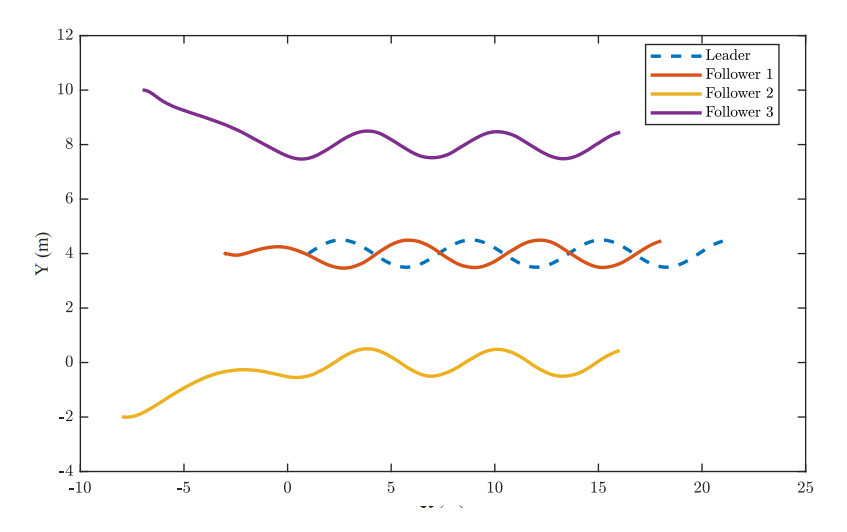
Figure 2. Positions of mobile robots using bioinspired distributed approach.

Neurodynamics- and observer-based distributed robust formation control for mobile robots

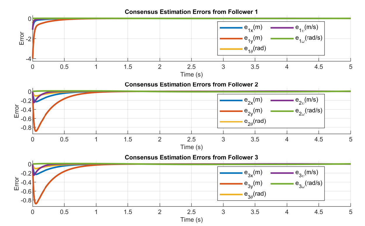
Figure 3. Consensus estimation error from the distributed estimator.

Neurodynamics- and observer-based distributed robust formation control for mobile robots

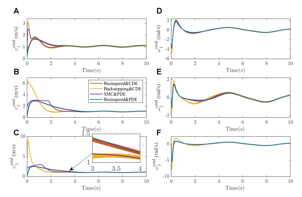
Figure 4. Velocity command generated from the velocity controller. (A-C) Linear velocity command; (D-F): Angular velocity command. CDE: Conventional distributed estimator; SMC: sliding mode control; PDE: proposed distributed estimator.

With the implementation of the neurodynamic-based controller, the speed jump issue is clearly avoided. If the initial tracking error in the driving direction is not zero, the velocity command will not be zero in the conventional approach. However, the bioinspired control method allows the initial velocity command to start from zero, allowing a lower torque command. Due to the bounded nature of the bioinspired neural dynamics, compared with the bioinspired method, the maximum velocity command from the conventional method reaches a maximum velocity of over 10m/s, which is apparently impractical.

Figure 5 illustrates the state estimation results obtained from the proposed nonlinear extended state observer. Since the velocity states are not directly measurable, the observer effectively reconstructs both the unmeasured states and external disturbances with high accuracy. As seen in Figure 5, the estimated disturbances closely match the true values, demonstrating the observer's strong estimation capability. Without this critical disturbance information, the overall formation performance would deteriorate significantly.

Neurodynamics- and observer-based distributed robust formation control for mobile robots

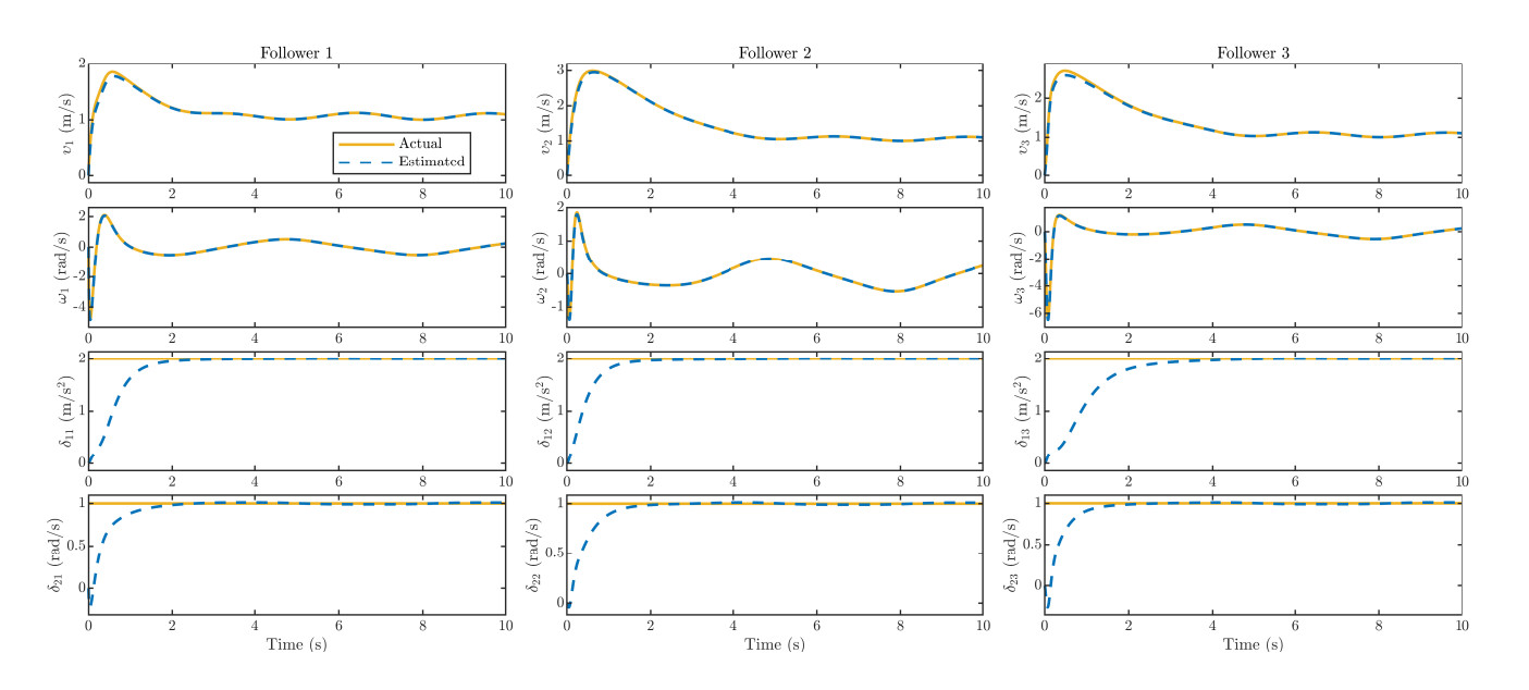
Figure 5. Velocity and disturbance estimates of each follower.

Moreover, the proposed nonlinear observer provides continuous and smooth state estimates, which enable the torque controller to generate smooth control inputs. Figure 6A-C compares the formation performance with and without the nonlinear state observer, showing that its inclusion leads to markedly improved tracking and formation stability. In Figure 6D-F, Gaussian-type noise is introduced into the inter-robot communication channels. Even under such noise, the proposed bio-inspired control law maintains smooth linear velocity outputs. This robustness arises from the bio-inspired neural dynamics given in Equation (35), which inherently act as a low-pass filter, effectively attenuating high-frequency noise and preserving continuous, noise-resilient control actions. As a result, the overall formation system exhibits improved robustness and smoother cooperative motion.

Neurodynamics- and observer-based distributed robust formation control for mobile robots

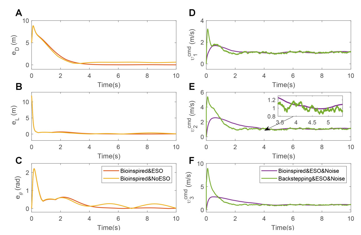
Figure 6. Tracking error with and without nonlinear state estimator (A) Tracking error in the driving direction; (B) Tracking error in the lateral direction; (C) Tracking error in the orientation; (D) Velocity command of Follower 1; (E) Velocity command of Follower 2; (F) Velocity command of Follower 3. ESO: Extended State Observer.

5. CONCLUSION

This work focuses on achieving robust formation coordination for multiple mobile robots in environments where velocity measurements are not directly accessible and external disturbances are present. To address these challenges, we construct an integrated control architecture combining distributed observation and biologically inspired coordination mechanisms. The strategy begins with a distributed estimation process that enables each robot to recover the leader's motion state continuously using only local communication. Building on these estimates, a bioinspired kinematic mechanism is introduced to generate smooth and bounded velocity commands, effectively mitigating abrupt transitions and enforcing motion constraints. To compensate for unknown dynamics and measurement uncertainties, a nonlinear observer is incorporated to estimate both actual velocities and disturbance terms. These inferred states are then fed into a robust torque-level controller tailored to maintain the formation under adverse conditions. Theoretical analysis confirms that the overall framework guarantees convergence and disturbance resilience, while numerical experiments illustrate that high-precision formation can be sustained even in the presence of significant uncertainty.

DECLARATION

Authors' contributions

Idea generation, algorithm design, and writing and editing of the original draft: Xu, Z.

Simulation and writing of the original draft: Xia, Z.

Supervision and feedback: Li, W.; Yang, S. X.

Availability of data and materials

The data supporting the conclusions of this article will be made available by the authors upon request.

AI and AI-assisted tools statement

During the preparation of this manuscript, the AI tool Chatgpt (Version 4.5, released 2025-02-27) was used solely for language editing. The tool did not influence the study design, data collection, analysis, interpretation, or the scientific content of the work.

Financial support and sponsorship

This work is supported by the Guangxi Zhuang Autonomous Region Key Research and Development Program (Project NO.AB22035023).

Conflict of interest

Yang, S. X. is the Editor-in-Chief of the journal Intelligence & Robotics. Yang, S. X. was not involved in any steps of the editorial process, notably including reviewer selection, manuscript handling, or decision-making. The other authors declare that there are no conflicts of interest.

Ethical approval and consent to participate

Not applicable.

Consent for publication

Not applicable.

Copyright

© The Author(s) 2026.

REFERENCES

1. Hu, J.; Liu, W.; Zhang, H.; Yi, J.; Xiong, Z. Multi-robot object transport motion planning with a deformable sheet. IEEE. Robot. Autom. Lett. 2022, 7, 9350-7.

2. Macwan, A.; Vilela, J.; Nejat, G.; Benhabib, B. A multirobot path-planning strategy for autonomous wilderness search and rescue. IEEE. Trans. Cybern. 2015, 45, 1784-97.

3. Lashkari, N.; Biglarbegian, M.; Yang, S. X. Development of a novel robust control method for formation of heterogeneous multiple mobile robots with autonomous docking capability. IEEE. Trans. Autom. Sci. Eng. 2020, 17, 1759-76.

4. Li, Q.; Zhuo, Z.; Gao, R.; et al. A pig behavior-tracking method based on a multi-channel high-efficiency attention mechanism. Agric. Commun. 2024, 2, 100062.

5. Wen, J.; Yang, J.; Li, Y.; He, J.; Li, Z.; Song, H. Behavior-based formation control digital twin for multi-AUG in edge computing. IEEE. Trans. Netw. Sci. Eng. 2023, 10, 2791-801.

6. Tan, G.; Zhuang, J.; Zou, J.; Wan, L. Coordination control for multiple unmanned surface vehicles using hybrid behavior-based method. Ocean. Eng. 2021, 232, 109147.

7. Bautista, J.; de Marina, H. G. Behavioral-based circular formation control for robot swarms. In 2024 IEEE International Conference on Robotics and Automation (ICRA), Yokohama, Japan, May 13-17, 2024. IEEE, 2024; pp. 8989–95.

8. Xu, Z.; Yan, T.; Yang, S. X.; Gadsden, S. A.; Biglarbegian, M. Distributed robust learning based formation control of mobile robots based on bioinspired neural dynamics. IEEE. Trans. Intell. Veh. 2024, 20, 1180-9.

9. Zhao, W.; Liu, H.; Lewis, F. L.; Wang, X. Data-driven optimal formation control for quadrotor team with unknown dynamics. IEEE. Trans. Cybern. 2022, 52, 7889-98.

10. Moorthy, S.; Joo, Y. H. Distributed leader-following formation control for multiple nonholonomic mobile robots via bioinspired neurodynamic approach. Neurocomputing 2022, 492, 308-21.

11. Guo, J.; Liu, Z.; Song, Y.; Yang, C.; Liang, C. Research on multi-UAV formation and semi-physical simulation with virtual structure. IEEE. Access. 2023, 11, 126027-39.

12. Villa, D. K. D.; Brandão, A. S.; Sarcinelli-Filho, M. Cooperative load transportation with quadrotors using adaptive RISE control. J. Intell. Robot. Syst. 2024, 110, 138.

13. Moreira, M. S. M.; Villa, D. K. D.; Sarcinelli-Filho, M. Controlling a virtual structure involving a UAV and a UGV for warehouse inventory. J. Intell. Robot. Syst. 2024, 110, 121.

14. Luo, D.; Wang, Y.; Li, Z.; Song, Y.; Lewis, F. L. Asymptotic leader-following consensus of heterogeneous multi-agent systems with unknown and time-varying control gains. IEEE. Trans. Autom. Sci. Eng. 2024, 22, 2768-79.

15. Li, B.; Gong, W.; Yang, Y.; Xiao, B. Distributed fixed-time leader-following formation control for multi-quadrotors with prescribed performance and collision avoidance. IEEE. Trans. Aerosp. Electro. Syst. 2023, 59, 7281-94.

16. Zhao, X. W.; Li, M. K.; Lai, Q.; Liu, Z. W. Neurodynamics-based formation tracking control of leader-follower nonholonomic multiagent systems. Intell. Robot. 2024, 4, 339-62.

17. Li, J.; Xu, Z.; Zhu, D.; et al. Bio-inspired intelligence with applications to robotics: a survey. Intell. Robot. 2021, 1, 58-83.

18. Hou, R.; Cui, L.; Bu, X.; Yang, J. Distributed formation control for multiple non-holonomic wheeled mobile robots with velocity constraint by using improved data-driven iterative learning. Appl. Math. Comput. 2021, 395, 125829.

19. Liu, Z. Q.; Ge, X.; Xie, H.; Han, Q. L.; Zheng, J.; Wang, Y. L. Secure leader-follower formation control of networked mobile robots under replay attacks. IEEE. Trans. Ind. Informatics. 2024, 20, 4149-59.

20. Han, Z.; Wang, W.; Ran, M.; Wen, C.; Wang, L. Switching-based distributed adaptive secure formation control for mobile robots with denial-of-service attacks. IEEE. Trans. Syst. Man. Cybern. Syst. 2024, 54, 4126-38.

21. Zhao, Z.; Li, X.; Liu, S.; Zhou, M.; Yang, X. Multi-mobile-robot transport and production integrated system optimization. IEEE. Trans. Autom. Sci. Eng. 2024, 22, 7480-91.

22. Rosenfelder, M.; Ebel, H.; Eberhard, P. Cooperative distributed nonlinear model predictive control of a formation of differentially-driven mobile robots. Robot. Auton. Syst. 2022, 150, 103993.

23. Peng, J.; Xiao, H.; Lai, G.; Chen, C. L. P. Consensus formation control of wheeled mobile robots with mixed disturbances under input constraints. J. Franklin. Inst. 2024, 361, 107300.

24. Chang, S.; Wang, Y.; Zuo, Z.; Yang, H. Fixed-time formation control for wheeled mobile robots with prescribed performance. IEEE. Trans. Control. Syst. Technol. 2022, 30, 844-51.

25. Yang, J.; Yu, H.; Xiao, F. Hybrid-triggered formation tracking control of mobile robots without velocity measurements. Int. J. Robust. Nonlinear. Control. 2022, 32, 1796-827.

26. Liu, W.; Wang, X.; Li, S. Formation control for leader-follower wheeled mobile robots based on embedded control technique. IEEE. Trans. Control. Syst. Technol. 2023, 31, 265-80.

27. Dai, S. L.; He, S.; Chen, X.; Jin, X. Adaptive leader-follower formation control of nonholonomic mobile robots with prescribed transient and steady-state performance. IEEE. Trans. Ind. Informat. 2020, 16, 3662-71.

28. Chen, M.; Ge, S. S.; Ren, B. Adaptive tracking control of uncertain MIMO nonlinear systems with input constraints. Automatica 2011, 47, 452-65.

29. Hodgkin, A. L.; Huxley, A. F. A quantitative description of membrane current and its application to conduction and excitation in nerve. Bull. Math. Biol. 1990, 52, 25-71.

Cite This Article

Research Article
Open Access
Neurodynamics- and observer-based distributed robust formation control for mobile robots

How to Cite

Download Citation

If you have the appropriate software installed, you can download article citation data to the citation manager of your choice. Simply select your manager software from the list below and click on download.

Export Citation File:

Type of Import

Tips on Downloading Citation

This feature enables you to download the bibliographic information (also called citation data, header data, or metadata) for the articles on our site.

Citation Manager File Format

Use the radio buttons to choose how to format the bibliographic data you're harvesting. Several citation manager formats are available, including EndNote and BibTex.

Type of Import

If you have citation management software installed on your computer your Web browser should be able to import metadata directly into your reference database.

Direct Import: When the Direct Import option is selected (the default state), a dialogue box will give you the option to Save or Open the downloaded citation data. Choosing Open will either launch your citation manager or give you a choice of applications with which to use the metadata. The Save option saves the file locally for later use.

Indirect Import: When the Indirect Import option is selected, the metadata is displayed and may be copied and pasted as needed.

About This Article

Disclaimer/Publisher’s Note: All statements, opinions, and data contained in this publication are solely those of the individual author(s) and contributor(s) and do not necessarily reflect those of OAE and/or the editor(s). OAE and/or the editor(s) disclaim any responsibility for harm to persons or property resulting from the use of any ideas, methods, instructions, or products mentioned in the content.
© The Author(s) 2026. Open Access This article is licensed under a Creative Commons Attribution 4.0 International License (https://creativecommons.org/licenses/by/4.0/), which permits unrestricted use, sharing, adaptation, distribution and reproduction in any medium or format, for any purpose, even commercially, as long as you give appropriate credit to the original author(s) and the source, provide a link to the Creative Commons license, and indicate if changes were made.

Data & Comments

Data

Views
69
Downloads
0
Citations
0
Comments
0
0

Comments

Comments must be written in English. Spam, offensive content, impersonation, and private information will not be permitted. If any comment is reported and identified as inappropriate content by OAE staff, the comment will be removed without notice. If you have any queries or need any help, please contact us at [email protected].

0
Download PDF
Share This Article
Scan the QR code for reading!
See Updates
Contents
Figures
Related
Intelligence & Robotics
ISSN 2770-3541 (Online)

Portico

All published articles are preserved here permanently:

https://www.portico.org/publishers/oae/

Portico

All published articles are preserved here permanently:

https://www.portico.org/publishers/oae/