


Intelligent and inclusive EEG-driven authentication for gender fairness and cognitive impairment
 0
0  , ...
, ... Abstract
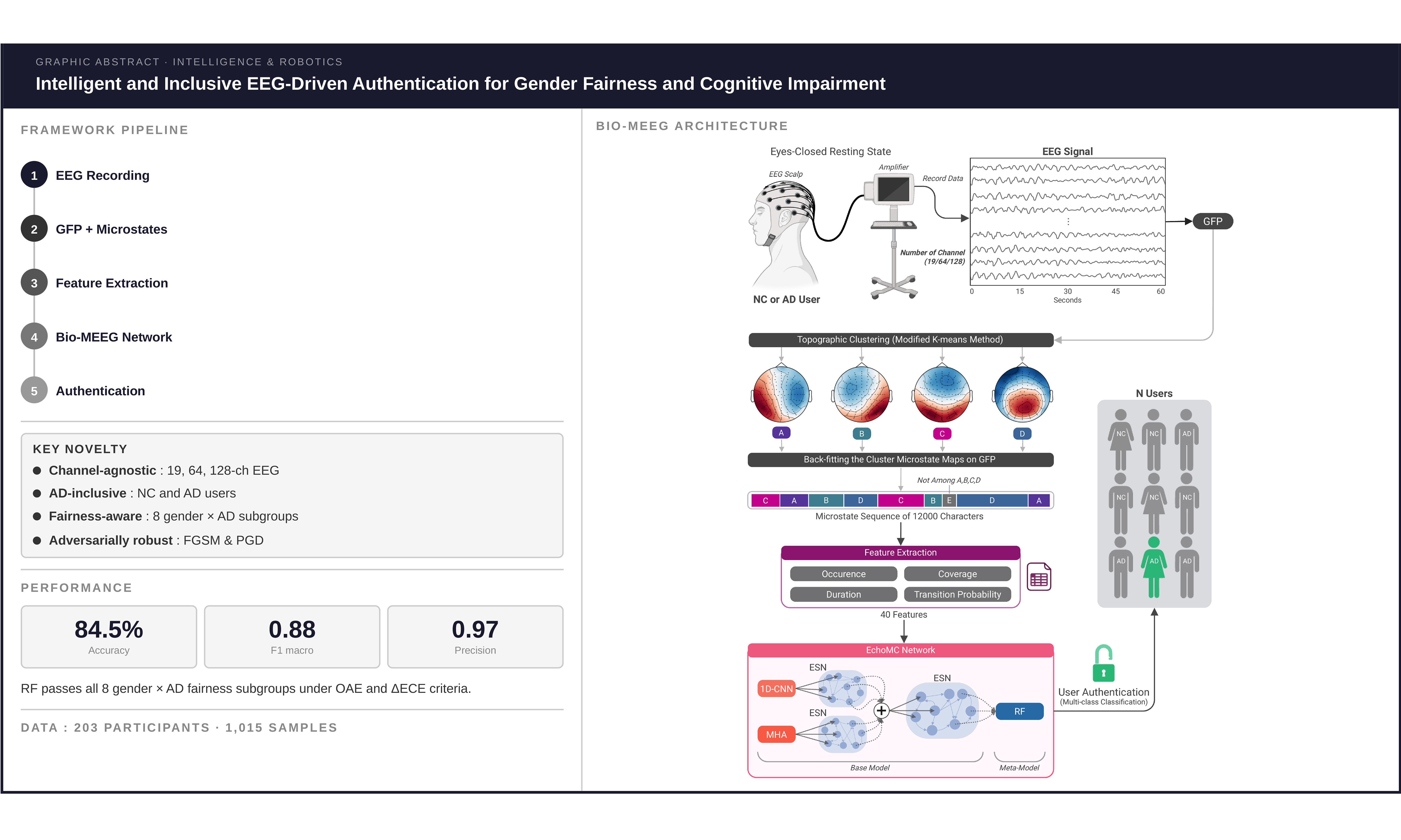
User authentication plays a key role in user modelling within computing systems, particularly for both normal control (NC) and Alzheimer’s disease (AD) users. Conventional authentication methods are vulnerable to external attacks and often rely on memory, which poses challenges for AD users experiencing cognitive decline. Electroencephalography (EEG) signals offer an alternative due to their subject-specific and difficult-to-replicate properties. However, differences in EEG patterns between NC and AD populations require intelligent authentication approaches that can generalise across heterogeneous user groups. This study proposes Biometric using microstates of EEG (Bio-MEEG), an intelligent EEG authentication framework that integrates EEG microstate analysis, one-dimensional convolutional neural networks (1D-CNNs), and ensemble learning based on echo state networks (ESNs) for user authentication under a closed-set, repeated-sample identification setting. The model is evaluated on 1,015 samples from 203 participants across multiple countries and EEG configurations. Results show that Bio-MEEG achieves stable authentication performance with minimal accuracy fluctuation across demographic subgroups and remains robust under feature-space adversarial perturbations. By supporting both NC and AD users without significant performance disparity, the proposed framework contributes toward more accessible, intelligent, and reliable EEG-based authentication systems.
Keywords
1. INTRODUCTION
User authentication in user modelling refers to verifying an individual’s or entity’s identity before granting access for users to systems, devices, or data[1-3]. Its primary aim is to ensure that access to specific resources is restricted to authorised users, thereby maintaining privacy and security[4]. Commonly used authentication methods include passwords, personal identification numbers (PINs), biometrics (such as fingerprints and facial recognition), smart cards, and tokens. Despite widespread use, these methods remain vulnerable to security breaches, such as using fake information or exploiting unique biometric traits. To address these challenges, researchers are actively exploring more advanced authentication techniques that offer higher levels of security. Existing authentication methods remain vulnerable to spoofing and data leakage, motivating the need for approaches that are harder to replicate or steal[5].
Recent research has highlighted the promising potential of utilising brain-computer interface (BCI)[6,7] with brain signals as a biometric authentication method, offering a fundamentally different approach based on neural signals rather than external identifiers[8]. Beyond authentication, BCI systems have been explored across a wide range of human--machine interaction contexts - including rehabilitation applications that integrate neural signals with physical actuation systems such as McKibben artificial muscles[9], demonstrating the versatility and growing maturity of BCI technology. The present work contributes to this ecosystem by advancing one of the most security-critical BCI applications: user authentication. One of the key biometric attributes utilised in BCI systems is the brain’s electrical activity, which is recorded through electroencephalography (EEG). EEG signals have garnered significant attention due to their appropriateness as a biometric method[10]. Unlike traditional biometric traits, EEG signals are highly secure. It cannot be captured by an external camera, such as facial or fingerprint biometrics, and does not rely on memorisation like passwords or PINs, removing the need for users to recall credentials. Moreover, EEG signals are intrinsic to the users and remain unaffected by changes in physical appearance. These notable characteristics, combined with their resistance to forgery, make EEG harder to replicate than surface biometrics such as face or fingerprint[11,12].
Furthermore, user authentication is not only essential for people without Alzheimer’s disease (AD)[13], often referred to as normal controls (NC)[14], but also for users with AD[15] (in this research, AD users may be referred to as mild AD that they generally might not need a guardian[16]). However, users with AD frequently experience progressive memory loss and cognitive decline[17], creating significant challenges in handling login credentials for essential services and increasing their vulnerability to cybercrime[18]. Hence, EEG-based authentication is especially relevant for this group because it removes the need to recall passwords, thereby reducing the risk of forgetting or unintentionally exposing sensitive information, such as written notes containing passwords, to unauthorised people. Nevertheless, EEG patterns of NC and AD users differ[19], highlighting the critical need for model generalisation in user authentication systems to ensure both groups achieve the same level of usability. Despite its importance, this issue is often overlooked, as evidenced by the limited number of studies addressing it in the literature.
AI models have made significant contributions to EEG-based authentication by effectively capturing complex patterns. However, the primary focus has been on improving model accuracy, typically neglecting the fairness of the developed methods. Evaluating and ensuring fairness in AI models for EEG-based authentication is crucial, as demographic biases, which can lead to unequal system performance and increase users’ exposure to security and privacy risks[20]. Gender, in particular, emerges as a critical factor, with evidence indicating that the underrepresentation of women during the development of AI models often leads to unintended biases[21]. This issue is particularly relevant in AI-based BCI systems using EEG, where biases in predictions are commonly reported[22]. Such biases negatively impact the usability and accessibility of these technologies, resulting in unfair AI models that fail to provide fairness systems to all users[23].
Building upon the direction and gaps mentioned above, the following are the key contributions of this research:
• Development of the BioMEEG Framework: Biometric using microstates of EEG (Bio-MEEG) leverages EEG microstates[24] as a generalisable approach based on EEG microstates for user authentication using multiple datasets from different countries compatible with a variety of channels. It advances and personalises an authentication technique for NC and AD users.
• Proposal of the EchoMC Network: Authenticating (classifying) participants’ EEG microstate patterns using ensemble learning with echo state network (ESN)[25], multi-head attention (MHA)[26] and one-dimensional convolutional neural network (1D-CNN)[27]. This component forms the core of the Bio-MEEG framework.
• Fairness with Multiple Sensitive Attributes and Robustness Assessment: Analysing and evaluating the EchoMC network with comprehensive fairness considerations with combined sensitive attributes and robustness evaluation, ensuring a fair and reliable model for users following trustworthy/human-centric AI core values[28].
2. RELATED WORK
To begin with, Chen et al. proposed an EEG-based authentication framework utilising ERP responses evoked by a rapid serial visual presentation (RSVP) paradigm[29]. Twenty-nine participants were involved, and their brain activity was recorded using 28 and 16 wet EEG electrodes, achieving single-trial classification accuracies of 87.8% ± 5.1% and 85.9% ± 5.0%, respectively. The system achieved an accuracy of 78.2% ± 5.7% using dry channels. Wu et al. implemented an EEG authentication system where participants focused on RSVP stimuli featuring faces[30]. The system recorded EEG attributes for login authentication and achieved a mean accuracy of 91.61% with data collected from 45 participants using 16 wet active channels. Meanwhile, Mu et al. introduced an authentication paradigm that differentiates between self-photos and non-self-photos[31]. The approach featured key innovations, including reducing display time, using fuzzy entropy (FE) for feature extraction instead of traditional temporal features, and adopting Back Propagation for classification, replacing the Gaussian support vector machine. This method, tested with data from 10 participants using two channels, achieved a classification accuracy of 87.3%. Another study by Wu et al. introduced an EEG authentication system incorporating eye-blinking signals[32]. This method integrates EEG and eye-blinking features via a self/non-self-face RSVP paradigm, extracts event-related potential (ERP) and morphological features, and employs convolutional neural network (CNN), Back Propagation, and least-squares fusion for score estimation, achieving 97.6% accuracy with data from 40 participants and 16 channels. Thomas and Vinod investigated EEG-based authentication using the PhysioNet database[33]. By focusing on gamma-band features and using power spectral density (PSD)-based feature extraction combined with Mahalanobis distance classification, they achieved a 90% accuracy rate using 19 EEG channels.
Next, Kumar et al. developed a multimodal system integrating EEG signals and dynamic signatures for mobile authentication[34]. The study involved 58 participants and 14 channels, employing a bidirectional long short-term memory neural network (BLSTM-NN) for classification and achieving an accuracy of 97.57%. Zeynali and Seyedarabi examined the use of a single-channel brainwave authentication system[35]. Using a discrete Fourier transform (DFT) and classification techniques such as SVM, Bayesian networks, and neural networks, their method achieved accuracies of 84.49%, 85.97%, and 92.89%, respectively, across 7 participants with 6 channels. Seha and Hatzinakos proposed a recognition approach based on steady-state auditory evoked potentials (AEPs)[36]. With 40 participants and 7 channels, the system achieved 96.46% accuracy by utilising canonical correlation analysis (CCA) for feature extraction and linear discriminant analysis (LDA) for classification. Rathi et al. developed an authentication system using a P300 speller paradigm[37]. This method, involving 10 participants and 10 channels, recorded an accuracy of 97%. Białas et al. presented a multifactor authentication system leveraging EEG signals[8]. Their system utilised AR for feature extraction and a fast forest classifier for classification, achieving an accuracy of 83.33%. Yap et al. evaluated transfer learning models for EEG authentication[38]. Using a dataset of 30 participants with 12 channels, the system achieved an accuracy range of 99.1%-99.9%. Similarly, Alsumari et al. proposed a deep CNN model for EEG-based authentication. With data from 30 to 109 participants using 1 to 64 channels, the method achieved a 99% accuracy, demonstrating its potential for real-world applications[39].
Recent advancements in EEG-based authentication have delivered promising results in enhancing accuracy. A study using a lightweight 1-D CNN model for motor imagery (MI) classification achieved 91.75% accuracy, demonstrating its potential for user authentication, especially for individuals with disabilities[40]. Another approach focused on ERPs (P300 and N400) and achieved an impressive equal error rate (EER) of 2.53% by utilising ensemble classifiers such as CatBoost and XGBoost[41]. To address challenges like cross-session recognition, a deep learning-based biometric verification system was proposed, combining fast Fourier transform (FFT) and convolutional autoencoder features (CAF). This method proved highly robust across diverse protocols[42]. Additionally, a CNN-BiLSTM (Bidirectional LSTM) model tackled noise and inter-subject variability, achieving 98.9% training accuracy and 92.2% validation accuracy[43].
Gap statements: Despite the high performance demonstrated by previous studies on EEG-based authentication, three critical gaps are identified from the literature. Firstly, fairness evaluation is overlooked, potentially resulting in biased predictions or unfair methods that are detrimental to users’ security and privacy. Secondly, current approaches only rely on a single dataset, limiting the generalisation of the model. Finally, the previous methods use data obtained from EEG systems with a fixed number of channels, which restrains the models’ adaptability to run across varying hardware setups and real-world settings.
3. MATERIALS
To address dataset-related gaps in the literature, this research aims to develop a generalizable model utilising four datasets from different countries with different numbers of channels for EEG authentication, all containing resting-state, eyes-closed EEG data with wet electrodes. This study is a retrospective analysis of publicly available EEG datasets. No proprietary EEG acquisition hardware was developed, and no original recording protocol was designed as part of this research. The contribution of Bio-MEEG lies in the proposed algorithmic pipeline, encompassing microstate-based feature extraction and the EchoMC stacking ensemble, evaluated on diverse, multi-country, multi-device datasets. Using established public datasets ensures reproducibility and enables benchmarking against prior work.
The framework is evaluated using a closed-set, repeated-sample identification setting. All participants in the test set are known during training. The task is to assign each EEG session to the correct registered user. This design reflects a realistic session-variability authentication scenario, asking “does this EEG recording still belong to this enrolled user across different time points?” rather than an open-set verification scenario where unknown users must be rejected. This distinction affects how the reported accuracy should be interpreted, as accuracy figures in closed-set paradigms are not directly comparable to EER figures reported in open-set studies. Subject-independent evaluation, where test participants are entirely unseen during training, represents an important and more demanding generalisation test that is planned as future work.
A detailed description of each dataset is provided below:
CHBMP [44] (https://portal.conp.ca/dataset?id=projects/CHBMP): This dataset comprises EEG recordings from a community-based population in La Lisa municipality, Havana, Cuba, focusing on young to middle-aged participants without neurological or brain disorders (i.e., NC). EEG data were recorded using 64 channels, and for this study, data from 19 NC participants are included.
DS004504 [45] (https://openneuro.org/datasets/ds004504/versions/1.0.9): Collected by neurologists at the Department of Neurology, AHEPA General Hospital in Thessaloniki, Greece, this dataset has EEG recordings with 19 channels. This research includes resting-state EEG data from 29 NC and 29 AD participants.
BrainLat [46] (https://www.synapse.org/Synapse:syn51549340/wiki/624187): This dataset was compiled across five South American countries (Argentina, Chile, Colombia, Mexico, and Peru) using a 128-channel Biosemi Active-Two acquisition system. For this study, data from a cohort of 30 NC and 27 AD participants were utilised.
PEARL-Neuro Database [47] (https://openneuro.org/datasets/ds004796/versions/1.1.0): Provided by the Laboratory of Emotions Neurobiology at the Nencki Institute of Experimental Biology PAS in Warsaw, Poland, this dataset used Brain Products systems, incorporating an actiCHamp amplifier and high-density actiCAP electrode caps with 128 channels (Brain Products GmbH, Munich, Germany). Data from 69 NC participants are included in this study.
The combined dataset includes 203 participants (147 NC and 56 AD) and 1,015 EEG samples, with each participant contributing five 60-second recordings. A common preprocessing step (resampling to 200 Hz and bandpass 2-20 Hz) was applied across all datasets, beyond which each dataset’s original source-specific preprocessing was retained[48,49]. More advanced preprocessing steps, such as ICA-based artefact removal, epoch rejection, and re-referencing, were not consistently applied. Instead, this study relies on the preprocessing and quality control procedures defined by the original dataset sources[44-47], which used dataset-specific protocols appropriate to their acquisition settings. As a result, residual artefacts (e.g., ocular or muscular activity) may persist unevenly across datasets, which is acknowledged as a limitation and motivates future work with a unified preprocessing pipeline.
The datasets also differ in acquisition hardware, including amplifier types, electrode configurations (active vs. passive), impedance standards, and reference schemes. No explicit cross-dataset harmonisation (e.g., ComBat) was applied beyond the shared preprocessing steps. However, the microstate feature extraction process provides partial robustness to such variability: global field power (GFP) is reference-independent and normalises spatial field strength, while global map dissimilarity (GMD) further standardises topographies by GFP before similarity computation. Consequently, derived microstate descriptors (occurrence, coverage, duration, and transitions) are largely invariant to amplitude scaling differences across devices. Nevertheless, residual biases due to differences in channel density (19 vs. 128 channels) and spatial sampling cannot be fully excluded and remain an inherent limitation of this multi-dataset design.
4. PROPOSED BIO-MEEG FRAMEWORK
4.1. EEG microstates
The EEG microstate approach models EEG signals as discrete, non-overlapping topographical patterns[24,50,51], which are linked back to the original data through spatial correlation techniques[52]. This method interprets EEG data as sequences of distinct topographies[53], and has been effectively applied in analysing differences in patterns in a variety of applications. Notably, it adapts varying EEG channels by standardising datasets into a consistent feature set, enabling the model to accept heterogeneous electrode configurations without architectural modification.
Figure 1 presents the microstate extraction workflow. The raw EEG signals collected by an amplifier (after pre-processing steps as detailed in Section 3) are then processed with GFP[54], computed for each time point using the following formula:
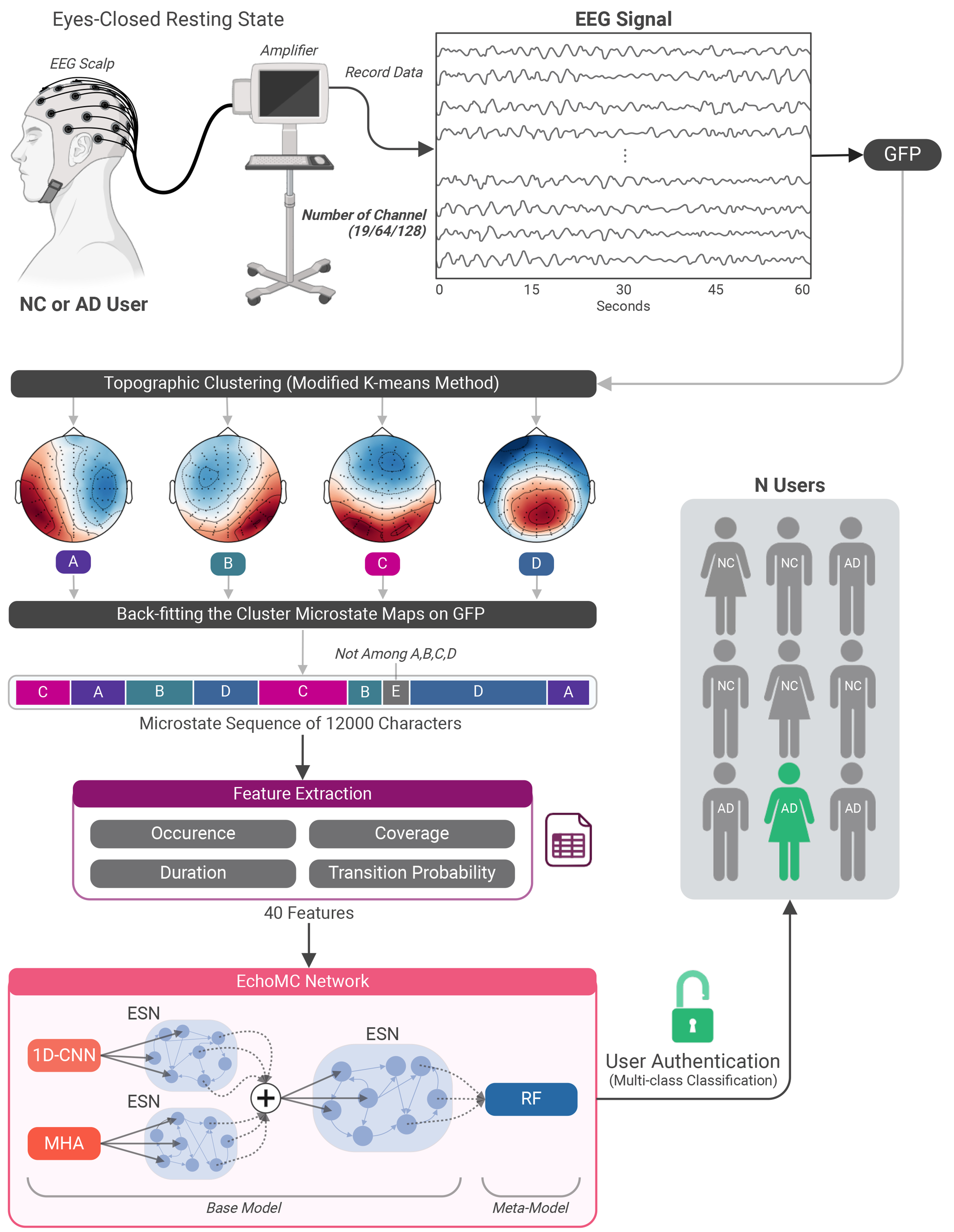
Figure 1. Bio-MEEG framework workflow. The icons used in Figure 1 are from MNE-Python (https://mne.tools/stable/credit.html) and BioRender (https://www.biorender.com/) for public use. Created in BioRender. N, Q. (2025) https://biorender.com/s97t212. Bio-MEEG: Biometric using microstates of electroencephalography; EEG: electroencephalography; NC: normal control; AD: Alzheimer’s disease; GFP: global field power; ESN: echo state network; MHA: multi-head attention; 1D-CNN: one-dimensional convolutional neural network; RF: random forest.
where
where u and v are topographical maps, and GFPu and GFPv are their corresponding GFP values. Four standard microstates (A, B, C, D) are identified, associated with key neural networks: auditory, visual, salience, and attention[56]. These microstates were then used to reconstruct the original EEG signal, forming the input sequence for the proposed model. It results in a sequence of 12,000 characters with A, B, C, D, or E (a small number of topographical maps that are unclassified among A, B, C, or D).
The microstate approach does not explicitly decompose EEG activity into anatomical brain regions (e.g., frontal vs. temporal). Instead, region-specific information is implicitly encoded in the topographic shape of each microstate: a frontally dominant topographic pattern will contribute positively to frontal-electrode GFP values and will be assigned to whichever microstate cluster best captures that spatial distribution. The four canonical microstates (A-D) are each associated with distinct distributed brain networks: auditory, visual, salience, and dorsal attention, respectively[57], which inherently involve different combinations of cortical regions. This approach allows the model to operate consistently across different numbers of EEG channels: the same microstate labels and feature set can be derived regardless of whether 19, 64, or 128 electrodes are used, at the cost of not providing region-specific interpretability.
A key property of the microstate pipeline is its natural reconciliation of heterogeneous channel configurations. Unlike conventional approaches that require a fixed-size input tensor corresponding to a specific electrode montage, the microstate framework operates as follows: GFP is computed across all available electrodes [Equation (1)] at each timepoint, whether 19, 64, or 128. Topographic clustering then identifies the dominant spatial patterns within each dataset’s electrode space independently. The resulting microstate sequence (A, B, C, D, E) is invariant to the number of input channels because it describes temporal patterns of dominant topography rather than specific electrode amplitudes. The 40 extracted features are therefore structurally identical across all four datasets, enabling joint model training and evaluation despite the heterogeneous hardware configurations.
As shown in Figure 1, this research utilises four essential EEG microstate properties as authenticating features: occurrence, coverage, duration, and transition probabilities. Occurrence represents the average frequency at which a particular microstate class is observed per second. Coverage denotes the proportion of time, expressed as a percentage, that a specific microstate class occupies within a second. Duration corresponds to the mean length of time a particular microstate class persists during a single occurrence. Transition probabilities measure the likelihood of shifting from one microstate class to another, capturing the dynamic changes and interactions between different brain states over time. To illustrate, consider microstate A. It is characterised by three primary features, occurrence, coverage, and duration, alongside its transition probabilities, which include transitions from A to A, A to B, A to C, A to D, and A to E. Together, these yield eight distinct features for microstate A. When extended to all four microstates (A, B, C, D) and E, this results in a total of 40 features serving as inputs for user authentication.
4.2. EchoMC network
4.2.1. Ensemble learning
Ensemble learning with stacking is utilised in this research to develop the proposed EchoMC network. Stacking is an ensemble learning technique that combines models, where the output of a base model(s) serves as input to another model, referred to as a meta-model, to make the final prediction of user authentication (multi-class classification), as depicted in Figure 1. This approach is adopted in this study due to its proven effectiveness in pattern recognition tasks[58].
4.2.2. MHA
The mechanism operates using three matrices: the query matrix (Q), the key matrix (K), and the value matrix (V). The result is a weighted sum of the values, where the attention mechanism determines the weights. The formula for scaled dot-product attention, originally introduced by Vaswani et al.[59], is Attention(Q, K, V) = softmax(
where each head headi is defined as:
The parameter matrices are specified as WiQ ∈
4.2.3. 1D-CNN
1D-CNN is an important component of the EchoMC network. It is chosen as a vital part because its effectiveness in understanding patterns of this technique has been proven in many studies, including AI models using EEG as input. In this research, with the input of 40 features, the input can be represented as a vector [x1, x2, …, x40], where each element corresponds to a unique feature. Following the standard convolutional formulation[60], a kernel (or filter) in 1D-CNN slides over this vector, identifying patterns and interactions between neighbouring features. The kernel is represented as a one-dimensional array of size k, with k defining the number of consecutive features processed at each step of the convolution. The kernel’s receptive field refers to the specific segment of k consecutive features it processes at a given position. As the kernel moves along the feature vector, it captures localised information by aggregating data from these adjacent features. For an input vector x and a kernel w, the convolution operation at a specific position t is calculated as:
In this context, x represents the input vector containing features, while w refers to the kernel applied during the convolution operation. The size of the kernel k determines the number of consecutive elements considered during each step. Specifically, x(t + i) represents the value of the input vector at position t + i, and w(i) corresponds to the value of the kernel at position i.
4.2.4. ESN
ESN[25] plays a key role in the proposed EchoMC network. As a prominent part of the reservoir computing paradigm[61], ESNs contribute significantly to the model’s capability to efficiently handle and process data. In the present EchoMC implementation, the ESN, like the 1D-CNN and MHA base learners, operates on the 40-dimensional microstate feature vector rather than directly on the 12,000-character microstate sequence. The ESN therefore functions as a randomly initialised non-linear projection in the reservoir-computing sense, whose high-dimensional internal state provides a rich representation that benefits downstream classification even when the input is non-sequential. While ESN is primarily recognised for its success in sequential data processing, they have also demonstrated strong performance in non-sequential classification tasks[62]. An ESN is defined by the tuple (Win, W, α), where Win and W are random matrices initialized based on predetermined parameters. The leaking rate α, an adjustable hyperparameter, is critical for optimising the network’s performance. When α = 1, leaky integration is disabled, resulting in the updated state
Unlike traditional deep learning models or fully connected layers, which involve training multiple layers of weights, ESN only adjusts the output weights Wout. During training, the network’s internal responses to the input are captured in a matrix R, referred to as the reservoir state matrix, where each column represents the state at a specific time step. The target outputs are stored in a matrix D. To compute the output weights Wout, ridge regression is applied:
where λ is the regularization parameter, and I represents the identity matrix. The inclusion of λ ensures that the output weights Wout are well-regularised, avoiding large values and enhancing the robustness of the model.
4.2.5. Meta-model
The random forest (RF) classifier is the meta-model in the EchoMC network to predict the outcome of user classification based on the output of the base model. RF is chosen for its effectiveness in pattern recognition[63] and its notable results in Section 6.1. RF employs weighted voting, where each decision tree’s contribution is scaled by an assigned weight wt, reflecting its accuracy. For an input x, each tree t produces a prediction ht(x), and the final class
5. EXPERIMENTS
5.1. Experimental pipeline
Firstly, regarding the validation approach, as described in Section 3, the dataset consists of 1,015 samples collected from 203 participants, with each participant contributing 5 samples. To illustrate, these can be denoted as S1, S2, S3, S4, and S5. For instance, participant I1 has his/her own S1, S2, S3, S4, and S5, and similarly for all other participants. We use ten validation splits so that all samples are evaluated.
In each split, two of the five samples from every participant are used for training, while the remaining three samples are reserved for testing. This ensures that the testing set in each split contains three of the five samples from every participant. Importantly, the assignment of samples to training or testing need not be identical across all participants. However, the ten splits must ensure that the training and testing samples for each participant differ across splits. For example, in the first split, S1 and S2 might be used for training while S3, S4, and S5 are used for testing. In subsequent splits, this allocation changes, maintaining the consistent 2:3 ratio while introducing diversity.
Each split’s testing phase has three test sets: one using normal samples and two additional sets generated through adversarial attacks. Model performance metrics are explained in Section 5.2, and fairness metrics (Section 5.3) are calculated for all test sets in every split. Finally, the results from all ten splits, the average and the standard deviation of the metrics, are reported to provide a comprehensive evaluation of model performance and fairness.
The adversarial robustness evaluation targets a white-box feature-space attack scenario. Specifically, the threat model assumes an adversary who: (a) has full knowledge of the trained EchoMC meta-model and its parameters; (b) operates at the feature level, i.e., perturbs the extracted 40-dimensional microstate feature vectors rather than raw EEG signals; and (c) aims to cause misclassification by applying minimal perturbations within an ℓ∞ ball of radius ϵ = 0.01, using fast gradient sign method (FGSM) and projected gradient descent (PGD). This simulates an attack targeting the feature representation rather than raw signals. Importantly, this threat model does not cover physical-domain attacks or hardware-level signal corruption. Non-adversarial stress tests (e.g., channel dropout, noise injection, site shift) were not conducted in this study but represent important future directions for validating robustness under realistic hardware variability.
5.2. Model performance evaluation metrics
To evaluate the developed model, five important metrics are employed: Accuracy, Recall (macro), Precision (macro), F1-score (macro), and expected calibration error (ECE) with a bin number of 10, following the reference studies[64]. Their values range from 0 to 1. Higher values indicate better models, except for ECE, where a lower value means a better model.
5.3. Fairness evaluation metrics
Rather than simply calculating metrics across the entire test set and reporting average results, fairness evaluation focuses on the demographic characteristics of the samples within the test sets. These demographic attributes, referred to as sensitive attributes[65], play a crucial role in assessing model fairness. In our research, sensitive attributes include Gender (male and female) and AD status (NC and AD), as we target to generalise the model for NC and AD users and gender-related biases in biometric model predictions are frequently observed[21]. This issue is particularly evident in AI-driven BCI systems using EEG[22].
To enable a more granular fairness evaluation, we move beyond examining a single sensitive attribute, such as comparing male vs. female or NC vs. AD independently. Instead, we consider multiple sensitive attributes simultaneously[65], considering combinations of these attributes. The comparisons are structured into eight groups within each test set and across each split: G1 compares NC and AD; G2 distinguishes between Male and Female participants; G3 contrasts Male NC with Male AD; G4 examines Male NC against Female NC; G5 compares Male NC with Female AD; G6 differentiates Male AD from Female AD; G7 contrasts Female NC with Male AD; and G8 examines Female NC vs. Female AD.
For transparency, the approximate subgroup sample sizes per split test set (3 samples per participant × number of participants) are as follows: Male NC participants: approximately 201 (67 participants × 3), Female NC participants: approximately 240 (80 participants × 3), Male AD participants: approximately 63 (21 participants × 3), and Female AD participants: approximately 105 (35 participants × 3). Note that exact counts vary slightly across splits due to the randomised 2:3 sample allocation. These counts inform the interpretation of overall accuracy equality (OAE) and calibration using ECE (ΔECE) values, as smaller subgroup sizes yield wider variance in the reported metrics, reflected in the standard deviations of the fairness results reported in Section 6.1.
About the fairness metrics, OAE and ΔECE are utilised for comprehensive evaluation. For example, consider a scenario where the results of model predictions for a specific split are available. These results include the sample index, ground truth labels, predicted labels, confidence scores, gender (male or female), and AD status (NC or AD). For group comparison G1, which compares sub-group A (NC) and sub-group B (AD), we first filter the data to calculate the Accuracy and ECE (as detailed in Section 5.2) for each sub-group separately. Next, we conduct a fairness evaluation by calculating the ratio of the difference between these two sub-groups using the following equations with results ranging from 0 to 1:
Lower OAE and ΔECE are better in fairness. This study adopts an acceptance threshold γ of 0.2, established by the “80% rule”[66] specifying that the performance of one group must reach at least 80% of the performance achieved by the other group.
5.4. Experimental setups
The hyperparameters of the EchoMC network, along with its meta-models, are detailed in Table 1. Notably, the hyperparameters for the meta-models and the models trained without the base model remain consistent across all methods used in this research. The selected meta-models were chosen based on their proven effectiveness in the literature[5]. Regarding the adversarial attacks, ϵ is set at 0.01. The software and libraries used in this study include the following: EEG microstate extraction was performed using the Pycrostates library[67]. Data visualisation was carried out using Matplotlib and Seaborn, while t-distributed stochastic neighbour embedding (t-SNE) was implemented using the scikit-learn library. To ensure full reproducibility, all hyperparameters for both base models and meta-models are reported in Table 1, and all software libraries used are listed above. No additional components beyond those described are required to replicate the experimental pipeline.
Models’ hyperparameters
| Model | Hyperparameter | Value |
| EchoMC Base Model | 1D-CNN filters | 8 |
| 1D-CNN kernel size | 3 | |
| 1D-CNN activation | relu | |
| MHA num heads | 4 | |
| MHA key dimension | 8 | |
| ESN layer 1 and 2 units | 32 | |
| ESN layer 1 and 2 ridge λ | 0.1 | |
| Final ESN units | 203 | |
| Final ESN ridge λ | 0.1 | |
| RF | n_estimators | 100 |
| criterion | gini | |
| max_depth | None | |
| min_samples_split | 2 | |
| min_samples_leaf | 1 | |
| XGBoost | eval_metric | logloss |
| use_label_encoder | False | |
| learning_rate | 0.3 | |
| max_depth | 6 | |
| n_estimators | 100 | |
| objective | binary:logistic | |
| DT | criterion | gini |
| splitter | best | |
| max_depth | None | |
| min_samples_split | 2 | |
| min_samples_leaf | 1 | |
| CatBoost | iterations | 1000 |
| learning_rate | 0.03 | |
| depth | 6 | |
| verbose | 0 | |
| loss_function | Logloss | |
| Gaussian NB | var_smoothing | 1e-09 |
| GBM | loss | log_loss |
| learning_rate | 0.1 | |
| n_estimators | 100 | |
| subsample | 1.0 | |
| criterion | friedman_mse | |
| max_depth | 3 | |
| k-NN | n_neighbors | 5 |
| weights | uniform | |
| algorithm | auto | |
| leaf_size | 30 | |
| p | 2 | |
| LightGBM | boosting_type | gbdt |
| num_leaves | 31 | |
| learning_rate | 0.1 | |
| n_estimators | 100 | |
| LR | penalty | l2 |
| dual | False | |
| tol | 1e-4 | |
| C | 1.0 | |
| fit_intercept | True | |
| max_iter | 1000 | |
| SVM | C | 1.0 |
| Kernel | rbf | |
| Degree | 3 | |
| Gamma | Scale | |
| Probability | True |
5.5. Statistical analysis
Detection of variations accounting for repeated measures
To assess changes in feature distributions across time points (irrespective of AD status), we applied the non-parametric Friedman test, which is well-suited for repeated measures without assuming normality. This allowed for the identification of temporal effects across sessions at the group level. To control for the multiplicity of comparisons and assess the significance of broader feature domains, we grouped related features into four categories, consisting of occurrence, coverage, duration, and transition - and combined P-values within each group using established statistical techniques.
Three methods were used for P-value combination: Fisher’s method[68], which aggregates P-values using the sum of their logarithms under the assumption of independence, yielding a chi-squared statistic; Stouffer’s method[69], which transforms P-values into z-scores and combines them within the standard normal distribution framework; and the Bonferroni correction[70], a conservative adjustment that scales individual P-values by the number of tests to control the family-wise error rate in the presence of potential dependencies.
Detection of variations based on AD status
To further investigate differences within each group, we stratified the data by AD status and repeated the same analysis for each subgroup (AD and NC). This stratified evaluation enabled the identification of intra-group temporal variations and facilitated a clearer understanding of how each group individually evolves.
Detection of variations over time and between AD and NC
To examine both time-dependent changes and group-specific effects simultaneously, we conducted a two-way repeated-measures analysis of variance (ANOVA) with one within-subjects factor (time) and one between-subjects factor (AD status). This analysis assessed the main effects of time, group, and their interaction, providing insight into whether temporal trends differed significantly between AD and NC groups. P-values resulting from these ANOVAs were again combined within the four predefined feature groups using Fisher’s, Stouffer’s, and Bonferroni’s methods, as described above. All analyses were implemented in Python using the scipy.stats and pingouin libraries[71].
To supplement statistical significance, effect sizes, specifically Kendall’s W for the Friedman tests and partial eta-squared (ηp2) for the two-way repeated measures ANOVA, are recommended as complementary measures of practical significance. Reporting these alongside the presented P-values in future extensions of this work would provide a standardised indication of effect magnitude independent of sample size, following best practice in statistical reporting[72].
Global hypothesis testing
The objective of the P-value combination strategies was to test the global null hypothesis {H0: ∩i=1kH0i}, which assumes that all individual null hypotheses H0i are true. Each pi corresponds to a feature-specific hypothesis.
Fisher’s method combines P-values assuming pi ~
where X2 ~ χ2(2k) under H0. The combined P-value is obtained as pc = 1 - F(X2, 2k), where F(·, 2k) denotes the cumulative distribution function of the chi-squared distribution with 2k degrees of freedom.
Stouffer’s method combines P-values by converting them into z-scores:
where Φ-1 is the inverse of the standard normal CDF, and z ~
Bonferroni’s method adjusts for multiple testing by conservatively scaling the smallest P-value:
This approach does not assume independence and effectively controls Type I error in the presence of correlated tests.
To supplement statistical significance, effect sizes are reported alongside P-values. For the two-way repeated measures ANOVA, partial eta-squared (ηp2) is computed as:
where values of 0.01, 0.06, and 0.14 correspond to small, medium, and large effects respectively. For the Friedman tests, Kendall’s W is reported as a measure of concordance across repeated samples, ranging from 0 (no agreement) to 1 (complete agreement). These effect size measures provide a standardised indication of practical significance independent of sample size.
5.6. Interpreting results of two-way repeated measures ANOVA
To interpret the results of the two-way repeated measures ANOVA, we focused primarily on the interaction effect between time and AD status. A significant interaction indicates that the effect of time on feature distributions differs between the AD and NC groups. In such cases, interpreting the main effects independently may be misleading, as group differences may be driven by divergent temporal patterns.
If the interaction term was not significant, we interpreted the main effects separately. A significant main effect of time suggests that feature values changed consistently over time across both groups. A significant main effect of group (AD vs. NC) indicates an overall difference in feature values between the two groups, averaged across time points.
This analytic framework allows us to disentangle group effects, temporal dynamics, and their interactions, facilitating a nuanced understanding of how cognitive status modulates changes in EEG-derived features over time.
6. RESULTS
6.1. Model performance and fairness
Regarding performance, Table 2 presents the results of various meta-models for the proposed EchoMC network. Among them, RF, along with XGBoost, DT, CatBoost, and LightGBM, achieved the highest accuracy and recall, both reaching 0.8446. Regarding F1-score, LightGBM leads with a score of 0.8820, indicating balanced performance across precision and recall. Notably, DT outperforms other models in precision, with a value of 0.9724, and achieves the lowest ECE of 5.92e-19, reflecting its high calibration performance. The most limited method is SVM, which has lower metrics than the others. However, it is vital to note that the gap between RF results and DT and LightGBM, achieving the highest precision and F1-score, is just 0.01% for both. When testing with adversarial attacks, with results in Table 3, the EchoMC network remains largely unaffected by these attacks.
EchoMC network performance: metrics with different meta-models across all splits on the normal test set
| Model | Accuracy ↑ | Precision ↑ | Recall ↑ | F1-Score ↑ | ECE ↓ |
| RF | 0.8446 ± 0.0383 | 0.9706 ± 0.0122 | 0.8446 ± 0.0383 | 0.8807 ± 0.0272 | 0.1371 ± 0.0068 |
| XGBoost | 0.8446 ± 0.0383 | 0.9706 ± 0.0135 | 0.8446 ± 0.0383 | 0.8810 ± 0.0280 | 0.2758 ± 0.0121 |
| DT | 0.8446 ± 0.0383 | 0.9724 ± 0.0109 | 0.8446 ± 0.0383 | 0.8814 ± 0.0279 | 5.92e-19 ± 1.17e-18 |
| CatBoost | 0.8422 ± 0.0376 | 0.9691 ± 0.0125 | 0.8422 ± 0.0376 | 0.8781 ± 0.0270 | 0.4974 ± 0.0151 |
| GNB | 0.4679 ± 0.0349 | 0.4704 ± 0.0607 | 0.4679 ± 0.0349 | 0.4464 ± 0.0425 | 0.5071 ± 0.0315 |
| GBM | 0.8446 ± 0.0383 | 0.9716 ± 0.0117 | 0.8446 ± 0.0383 | 0.8812 ± 0.0277 | 1.04e-06 ± 3.24e-07 |
| k-NN | 0.3399 ± 0.0203 | 0.2856 ± 0.0247 | 0.3399 ± 0.0203 | 0.2834 ± 0.0213 | 0.0661 ± 0.0151 |
| LightGBM | 0.8446 ± 0.0383 | 0.9697 ± 0.0123 | 0.8446 ± 0.0383 | 0.8820 ± 0.0276 | 0.0014 ± 0.0003 |
| LR | 0.4449 ± 0.0454 | 0.4627 ± 0.0748 | 0.4449 ± 0.0454 | 0.4264 ± 0.0564 | 0.3005 ± 0.0264 |
| SVM | 0.2840 ± 0.0307 | 0.2282 ± 0.0362 | 0.2840 ± 0.0307 | 0.2295 ± 0.0357 | 0.2742 ± 0.0313 |
EchoMC network performance: metrics with different meta-models across all splits on test sets with adversarial attacks (FGSM, PGD)
| Model | Test set | Accuracy ↑ | Precision ↑ | Recall ↑ | F1-Score ↑ | ECE ↓ |
| RF | PGD | 0.8446 ± 0.0383 | 0.9707 ± 0.0121 | 0.8446 ± 0.0383 | 0.8806 ± 0.0272 | 0.1370 ± 0.0069 |
| FGSM | 0.8446 ± 0.0383 | 0.9707 ± 0.0122 | 0.8446 ± 0.0383 | 0.8806 ± 0.0272 | 0.1371 ± 0.0069 | |
| XGBoost | PGD | 0.8446 ± 0.0383 | 0.9708 ± 0.0128 | 0.8446 ± 0.0383 | 0.8815 ± 0.0276 | 0.2748 ± 0.0128 |
| FGSM | 0.8446 ± 0.0383 | 0.9703 ± 0.0124 | 0.8446 ± 0.0383 | 0.8812 ± 0.0277 | 0.2756 ± 0.0125 | |
| DT | PGD | 0.8449 ± 0.0383 | 0.9724 ± 0.0109 | 0.8449 ± 0.0383 | 0.8816 ± 0.0279 | 5.92e-19 ± 1.17e-18 |
| FGSM | 0.8449 ± 0.0383 | 0.9724 ± 0.0109 | 0.8449 ± 0.0383 | 0.8816 ± 0.0279 | 5.92e-19 ± 1.17e-18 | |
| CatBoost | PGD | 0.8426 ± 0.0384 | 0.9691 ± 0.0128 | 0.8426 ± 0.0384 | 0.8786 ± 0.0278 | 0.4981 ± 0.0175 |
| FGSM | 0.8426 ± 0.0384 | 0.9690 ± 0.0130 | 0.8426 ± 0.0384 | 0.8784 ± 0.0278 | 0.4994 ± 0.0167 | |
| GNB | PGD | 0.4679 ± 0.0349 | 0.4704 ± 0.0607 | 0.4679 ± 0.0349 | 0.4464 ± 0.0425 | 0.5071 ± 0.0315 |
| FGSM | 0.4679 ± 0.0349 | 0.4704 ± 0.0607 | 0.4679 ± 0.0349 | 0.4464 ± 0.0425 | 0.5071 ± 0.0315 | |
| GBM | PGD | 0.8446 ± 0.0383 | 0.9715 ± 0.0117 | 0.8446 ± 0.0383 | 0.8814 ± 0.0277 | 1.04e-06 ± 3.26e-07 |
| FGSM | 0.8446 ± 0.0383 | 0.9716 ± 0.0117 | 0.8446 ± 0.0383 | 0.8812 ± 0.0277 | 1.04e-06 ± 3.21e-07 | |
| k-NN | PGD | 0.3399 ± 0.0203 | 0.2856 ± 0.0246 | 0.3399 ± 0.0203 | 0.2834 ± 0.0213 | 0.0661 ± 0.0151 |
| FGSM | 0.3399 ± 0.0203 | 0.2854 ± 0.0247 | 0.3399 ± 0.0203 | 0.2834 ± 0.0213 | 0.0661 ± 0.0151 | |
| LightGBM | PGD | 0.8446 ± 0.0383 | 0.9700 ± 0.0121 | 0.8446 ± 0.0383 | 0.8821 ± 0.0276 | 0.0014 ± 0.0003 |
| FGSM | 0.8446 ± 0.0383 | 0.9697 ± 0.0123 | 0.8446 ± 0.0383 | 0.8820 ± 0.0276 | 0.0014 ± 0.0003 | |
| LR | PGD | 0.4448 ± 0.0459 | 0.4633 ± 0.0737 | 0.4448 ± 0.0459 | 0.4266 ± 0.0560 | 0.3000 ± 0.0269 |
| FGSM | 0.4456 ± 0.0448 | 0.4648 ± 0.0723 | 0.4456 ± 0.0448 | 0.4277 ± 0.0548 | 0.3004 ± 0.0256 | |
| SVM | PGD | 0.2840 ± 0.0307 | 0.2282 ± 0.0362 | 0.2840 ± 0.0307 | 0.2295 ± 0.0357 | 0.2740 ± 0.0316 |
| FGSM | 0.2840 ± 0.0307 | 0.2282 ± 0.0362 | 0.2840 ± 0.0307 | 0.2295 ± 0.0357 | 0.2738 ± 0.0305 |
It is important to be precise about what Table 4 demonstrates and what it does not. Table 4 shows that meta-models trained directly on the 40 microstate features, without the EchoMC base model, achieve accuracy below 0.35 across all meta-models, confirming that the stacked ensemble structure is essential and that neither the meta-model choice nor the microstate features alone are sufficient for strong performance. This provides evidence that the gain is attributable to the learned intermediate representations produced by the EchoMC base model. However, Table 4 does not isolate: (a) the contribution of microstate features relative to conventional EEG features such as band-power or connectivity measures; (b) the individual contributions of MHA, 1D-CNN, and ESN as standalone classifiers; or (c) the stacked architecture relative to a non-stacked deep baseline of equivalent capacity. These ablations are necessary to fully attribute the observed gains and are committed to as future work.
Machine learning models’ performance without a base model (ensemble learning)
| Model | Accuracy ↑ | Precision ↑ | Recall ↑ | F1-Score ↑ | ECE ↓ |
| RF | 0.3266 ± 0.0155 | 0.3266 ± 0.0155 | 0.3266 ± 0.0155 | 0.3266 ± 0.0155 | 0.1056 ± 0.0172 |
| XGBoost | 0.2538 ± 0.0205 | 0.2538 ± 0.0205 | 0.2538 ± 0.0205 | 0.2538 ± 0.0205 | 0.0735 ± 0.0203 |
| DT | 0.2023 ± 0.0245 | 0.2023 ± 0.0245 | 0.2023 ± 0.0245 | 0.2023 ± 0.0245 | 0.6548 ± 0.0400 |
| CatBoost | 0.3147 ± 0.0132 | 0.3147 ± 0.0132 | 0.3147 ± 0.0132 | 0.3147 ± 0.0132 | 0.2508 ± 0.0127 |
| GNB | 0.0993 ± 0.0122 | 0.0993 ± 0.0122 | 0.0993 ± 0.0122 | 0.0993 ± 0.0122 | 0.8489 ± 0.0245 |
| GBM | 0.1298 ± 0.0065 | 0.1298 ± 0.0065 | 0.1298 ± 0.0065 | 0.1298 ± 0.0065 | 0.4329 ± 0.0204 |
| k-NN | 0.1469 ± 0.0104 | 0.1469 ± 0.0104 | 0.1469 ± 0.0104 | 0.1469 ± 0.0104 | 0.1321 ± 0.0100 |
| LightGBM | 0.2077 ± 0.0157 | 0.2077 ± 0.0157 | 0.2077 ± 0.0157 | 0.2077 ± 0.0157 | 0.2557 ± 0.0331 |
| LR | 0.3080 ± 0.0243 | 0.3080 ± 0.0243 | 0.3080 ± 0.0243 | 0.3080 ± 0.0243 | 0.1690 ± 0.0475 |
| SVM | 0.1996 ± 0.0194 | 0.1996 ± 0.0194 | 0.1996 ± 0.0194 | 0.1996 ± 0.0194 | 0.1886 ± 0.0192 |
About fairness, as observed in Table 5 and Figure 2, all meta-models demonstrate fairness with the OAE metric, except GNB, k-NN, LR, and SVM. This trend is the same regardless of testing on regular or adversarial attacks [Table 6]. These four models exhibit the lowest performance metrics, as shown in Table 2. This suggests a potential relationship between lower predictive performance and increased unfairness in model outcomes. However, when evaluating fairness using calibration (ΔECE) with normal and adversarial attacks, as detailed in Table 7 with Figure 3 and Table 8, respectively, it reveals that only RF achieves fairness across all groups, with no group exceeding the acceptance threshold γ of 0.2. Therefore, although RF does not achieve the highest performance metrics, its ability to maintain fairness while delivering competitive performance results makes it the preferred meta-model among those evaluated as the meta-model for the proposed EchoMC network.
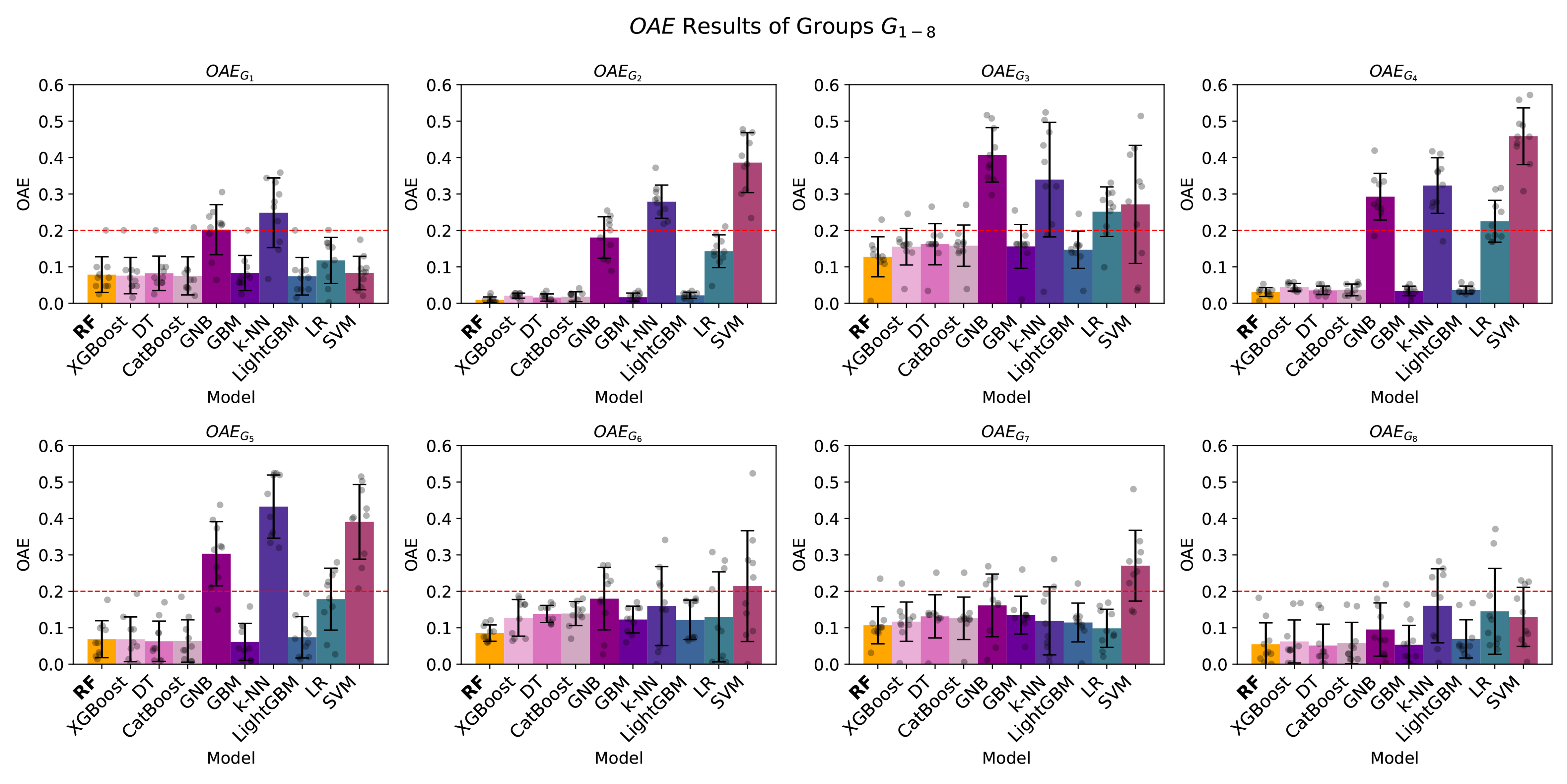
Figure 2. EchoMC network fairness visualisation: OAE with groups G1-8 of different meta-models across all splits. Error bars represent the standard deviation of OAE across the n = 10 validation splits. The dashed red line indicates the acceptance threshold γ = 0.2. OAE: Overall accuracy equality; RF: random forest; XGBoost: eXtreme gradient boosting; DT: decision tree; CatBoost: categorical boosting; GNB: Gaussian naive Bayes; GBM: gradient boosting machine; k-NN: k-nearest neighbors; LightGBM: light gradient boosting machine; LR: logistic regression; SVM: support vector machine.
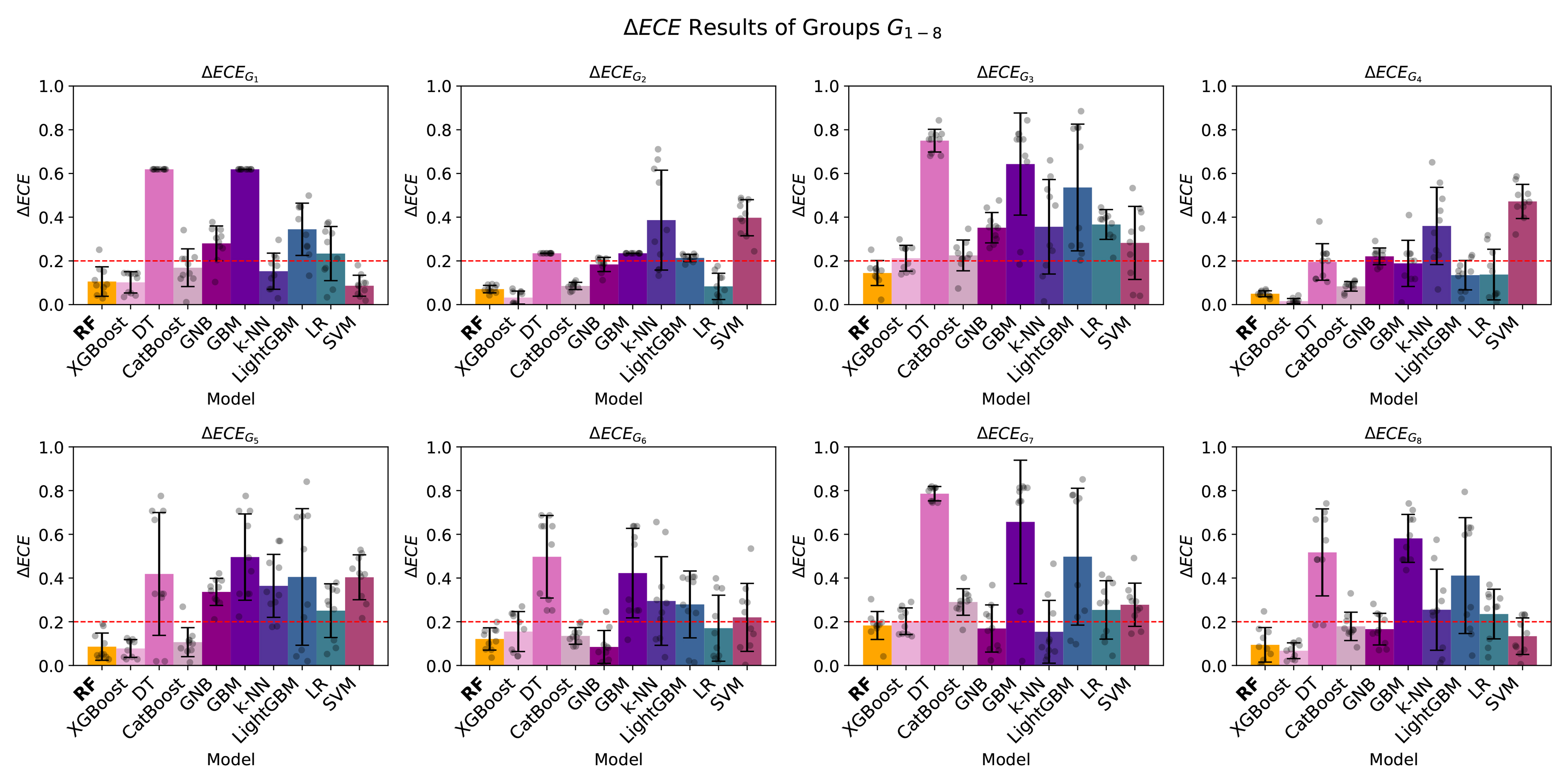
Figure 3. EchoMC network fairness visualisation: ΔECE with groups G1-8 of different meta-models across all splits. Error bars represent the standard deviation of ΔECE across the n = 10 validation splits. The dashed red line indicates the acceptance threshold γ = 0.2. ΔECE: Calibration using expected calibration error; RF: random forest; XGBoost: eXtreme gradient boosting; DT: decision tree; CatBoost: categorical boosting; GNB: Gaussian naive Bayes; GBM: gradient boosting machine; k-NN: k-nearest neighbors; LightGBM: light gradient boosting machine; LR: logistic regression; SVM: support vector machine.
EchoMC network fairness: OAE with groups G1-8: different meta-models across all splits on the normal test set
| Model | | | | | | | | |
| RF | 0.079 ± 0.049 | 0.010 ± 0.008 | 0.128 ± 0.055 | 0.031 ± 0.012 | 0.069 ± 0.051 | 0.085 ± 0.022 | 0.107 ± 0.051 | 0.055 ± 0.059 |
| XGBoost | 0.076 ± 0.050 | 0.021 ± 0.007 | 0.155 ± 0.050 | 0.044 ± 0.011 | 0.068 ± 0.061 | 0.127 ± 0.050 | 0.117 ± 0.054 | 0.062 ± 0.059 |
| DT | 0.082 ± 0.047 | 0.016 ± 0.010 | 0.162 ± 0.057 | 0.035 ± 0.012 | 0.063 ± 0.055 | 0.138 ± 0.024 | 0.131 ± 0.059 | 0.051 ± 0.059 |
| CatBoost | 0.075 ± 0.052 | 0.018 ± 0.014 | 0.158 ± 0.057 | 0.037 ± 0.016 | 0.064 ± 0.058 | 0.139 ± 0.033 | 0.126 ± 0.058 | 0.058 ± 0.057 |
| GNB | 0.202 ± 0.069 | 0.181 ± 0.057 | 0.407 ± 0.075 | 0.293 ± 0.064 | 0.303 ± 0.088 | 0.180 ± 0.086 | 0.161 ± 0.086 | 0.095 ± 0.073 |
| GBM | 0.083 ± 0.048 | 0.017 ± 0.011 | 0.156 ± 0.060 | 0.034 ± 0.013 | 0.061 ± 0.051 | 0.123 ± 0.037 | 0.135 ± 0.052 | 0.053 ± 0.053 |
| k-NN | 0.248 ± 0.096 | 0.279 ± 0.046 | 0.340 ± 0.157 | 0.323 ± 0.076 | 0.433 ± 0.087 | 0.160 ± 0.108 | 0.119 ± 0.093 | 0.160 ± 0.102 |
| LightGBM | 0.074 ± 0.052 | 0.022 ± 0.009 | 0.147 ± 0.051 | 0.037 ± 0.011 | 0.074 ± 0.057 | 0.122 ± 0.054 | 0.114 ± 0.053 | 0.069 ± 0.052 |
| LR | 0.118 ± 0.063 | 0.143 ± 0.045 | 0.251 ± 0.068 | 0.225 ± 0.057 | 0.178 ± 0.084 | 0.129 ± 0.123 | 0.098 ± 0.052 | 0.145 ± 0.117 |
| SVM | 0.083 ± 0.046 | 0.386 ± 0.082 | 0.271 ± 0.162 | 0.459 ± 0.078 | 0.391 ± 0.103 | 0.214 ± 0.152 | 0.270 ± 0.097 | 0.130 ± 0.081 |
EchoMC network OAE with groups G1-8: different meta-models across all splits on test sets with adversarial attacks (FGSM, PGD)
| Model | Test set | | | | | | | | |
| RF | PGD | 0.075 ± 0.049 | 0.011 ± 0.007 | 0.134 ± 0.064 | 0.036 ± 0.010 | 0.061 ± 0.049 | 0.097 ± 0.029 | 0.111 ± 0.054 | 0.051 ± 0.049 |
| FGSM | 0.080 ± 0.047 | 0.008 ± 0.006 | 0.133 ± 0.058 | 0.035 ± 0.011 | 0.068 ± 0.052 | 0.089 ± 0.015 | 0.108 ± 0.049 | 0.047 ± 0.058 | |
| XGBoost | PGD | 0.075 ± 0.050 | 0.019 ± 0.007 | 0.153 ± 0.050 | 0.042 ± 0.009 | 0.065 ± 0.062 | 0.126 ± 0.047 | 0.116 ± 0.054 | 0.060 ± 0.060 |
| FGSM | 0.076 ± 0.050 | 0.017 ± 0.009 | 0.158 ± 0.050 | 0.041 ± 0.011 | 0.064 ± 0.061 | 0.135 ± 0.045 | 0.122 ± 0.053 | 0.064 ± 0.057 | |
| DT | PGD | 0.083 ± 0.047 | 0.016 ± 0.010 | 0.162 ± 0.057 | 0.035 ± 0.012 | 0.063 ± 0.055 | 0.137 ± 0.023 | 0.131 ± 0.059 | 0.050 ± 0.059 |
| FGSM | 0.083 ± 0.047 | 0.016 ± 0.010 | 0.162 ± 0.057 | 0.035 ± 0.012 | 0.063 ± 0.055 | 0.137 ± 0.023 | 0.131 ± 0.059 | 0.050 ± 0.059 | |
| CatBoost | PGD | 0.073 ± 0.050 | 0.018 ± 0.011 | 0.154 ± 0.059 | 0.037 ± 0.012 | 0.061 ± 0.052 | 0.135 ± 0.039 | 0.122 ± 0.062 | 0.058 ± 0.050 |
| FGSM | 0.075 ± 0.052 | 0.019 ± 0.013 | 0.155 ± 0.065 | 0.036 ± 0.014 | 0.062 ± 0.053 | 0.136 ± 0.036 | 0.127 ± 0.063 | 0.056 ± 0.053 | |
| GNB | PGD | 0.202 ± 0.069 | 0.181 ± 0.057 | 0.407 ± 0.075 | 0.293 ± 0.064 | 0.303 ± 0.088 | 0.180 ± 0.086 | 0.161 ± 0.086 | 0.095 ± 0.073 |
| FGSM | 0.202 ± 0.069 | 0.181 ± 0.057 | 0.407 ± 0.075 | 0.293 ± 0.064 | 0.303 ± 0.088 | 0.180 ± 0.086 | 0.161 ± 0.086 | 0.095 ± 0.073 | |
| GBM | PGD | 0.087 ± 0.047 | 0.016 ± 0.009 | 0.165 ± 0.055 | 0.035 ± 0.012 | 0.067 ± 0.055 | 0.133 ± 0.032 | 0.134 ± 0.059 | 0.061 ± 0.051 |
| FGSM | 0.082 ± 0.046 | 0.013 ± 0.010 | 0.159 ± 0.056 | 0.034 ± 0.009 | 0.063 ± 0.051 | 0.131 ± 0.030 | 0.129 ± 0.061 | 0.050 ± 0.057 | |
| k-NN | PGD | 0.248 ± 0.096 | 0.279 ± 0.046 | 0.340 ± 0.157 | 0.323 ± 0.076 | 0.433 ± 0.087 | 0.160 ± 0.108 | 0.119 ± 0.093 | 0.160 ± 0.102 |
| FGSM | 0.248 ± 0.096 | 0.279 ± 0.046 | 0.340 ± 0.157 | 0.323 ± 0.076 | 0.433 ± 0.087 | 0.160 ± 0.108 | 0.119 ± 0.093 | 0.160 ± 0.102 | |
| LightGBM | PGD | 0.075 ± 0.051 | 0.021 ± 0.008 | 0.148 ± 0.051 | 0.037 ± 0.010 | 0.072 ± 0.058 | 0.121 ± 0.053 | 0.114 ± 0.053 | 0.068 ± 0.053 |
| FGSM | 0.074 ± 0.052 | 0.021 ± 0.008 | 0.148 ± 0.051 | 0.038 ± 0.010 | 0.073 ± 0.057 | 0.122 ± 0.054 | 0.114 ± 0.053 | 0.070 ± 0.053 | |
| LR | PGD | 0.113 ± 0.053 | 0.146 ± 0.044 | 0.247 ± 0.052 | 0.224 ± 0.059 | 0.171 ± 0.093 | 0.117 ± 0.114 | 0.082 ± 0.050 | 0.139 ± 0.105 |
| FGSM | 0.115 ± 0.054 | 0.147 ± 0.043 | 0.245 ± 0.064 | 0.223 ± 0.056 | 0.174 ± 0.097 | 0.131 ± 0.107 | 0.086 ± 0.050 | 0.137 ± 0.108 | |
| SVM | PGD | 0.083 ± 0.046 | 0.386 ± 0.082 | 0.271 ± 0.162 | 0.459 ± 0.078 | 0.391 ± 0.103 | 0.214 ± 0.152 | 0.270 ± 0.097 | 0.130 ± 0.081 |
| FGSM | 0.083 ± 0.046 | 0.386 ± 0.082 | 0.271 ± 0.162 | 0.459 ± 0.078 | 0.391 ± 0.103 | 0.214 ± 0.152 | 0.270 ± 0.097 | 0.130 ± 0.081 |
EchoMC network fairness: ΔECE with groups G1-8: different meta-models across all splits on the normal test set
| Model | | | | | | | | |
| RF | 0.106 ± 0.067 | 0.071 ± 0.017 | 0.145 ± 0.057 | 0.050 ± 0.014 | 0.086 ± 0.062 | 0.121 ± 0.051 | 0.183 ± 0.064 | 0.094 ± 0.079 |
| XGBoost | 0.102 ± 0.049 | 0.032 ± 0.030 | 0.212 ± 0.059 | 0.016 ± 0.012 | 0.078 ± 0.041 | 0.155 ± 0.091 | 0.202 ± 0.061 | 0.067 ± 0.036 |
| DT | 0.619 ± 0.000 | 0.235 ± 0.000 | 0.750 ± 0.052 | 0.195 ± 0.084 | 0.419 ± 0.281 | 0.497 ± 0.189 | 0.786 ± 0.033 | 0.517 ± 0.199 |
| CatBoost | 0.169 ± 0.086 | 0.085 ± 0.017 | 0.225 ± 0.070 | 0.083 ± 0.022 | 0.107 ± 0.066 | 0.135 ± 0.038 | 0.290 ± 0.061 | 0.179 ± 0.065 |
| GNB | 0.280 ± 0.080 | 0.184 ± 0.033 | 0.352 ± 0.069 | 0.221 ± 0.038 | 0.337 ± 0.062 | 0.085 ± 0.075 | 0.169 ± 0.108 | 0.166 ± 0.072 |
| GBM | 0.619 ± 0.000 | 0.235 ± 0.000 | 0.643 ± 0.234 | 0.189 ± 0.106 | 0.496 ± 0.197 | 0.423 ± 0.205 | 0.657 ± 0.282 | 0.581 ± 0.110 |
| k-NN | 0.153 ± 0.083 | 0.387 ± 0.229 | 0.356 ± 0.216 | 0.360 ± 0.177 | 0.364 ± 0.144 | 0.295 ± 0.203 | 0.154 ± 0.144 | 0.255 ± 0.185 |
| LightGBM | 0.345 ± 0.120 | 0.214 ± 0.016 | 0.536 ± 0.290 | 0.135 ± 0.067 | 0.405 ± 0.313 | 0.279 ± 0.153 | 0.498 ± 0.313 | 0.411 ± 0.265 |
| LR | 0.233 ± 0.123 | 0.083 ± 0.060 | 0.366 ± 0.068 | 0.137 ± 0.115 | 0.250 ± 0.122 | 0.170 ± 0.151 | 0.251 ± 0.133 | 0.235 ± 0.113 |
| SVM | 0.086 ± 0.048 | 0.397 ± 0.083 | 0.282 ± 0.167 | 0.472 ± 0.078 | 0.403 ± 0.103 | 0.220 ± 0.156 | 0.278 ± 0.099 | 0.134 ± 0.084 |
EchoMC network ΔECE with groups G1-8: different meta-models across all splits on test sets with adversarial attacks (FGSM, PGD)
| Model | Test set | | | | | | | | |
| RF | PGD | 0.101 ± 0.053 | 0.076 ± 0.019 | 0.157 ± 0.068 | 0.055 ± 0.029 | 0.073 ± 0.051 | 0.134 ± 0.031 | 0.194 ± 0.080 | 0.093 ± 0.059 |
| FGSM | 0.109 ± 0.056 | 0.083 ± 0.019 | 0.146 ± 0.060 | 0.060 ± 0.022 | 0.065 ± 0.059 | 0.140 ± 0.026 | 0.195 ± 0.066 | 0.089 ± 0.061 | |
| XGBoost | PGD | 0.102 ± 0.049 | 0.033 ± 0.027 | 0.212 ± 0.053 | 0.016 ± 0.012 | 0.087 ± 0.049 | 0.144 ± 0.091 | 0.201 ± 0.060 | 0.078 ± 0.044 |
| FGSM | 0.103 ± 0.048 | 0.033 ± 0.027 | 0.227 ± 0.055 | 0.016 ± 0.011 | 0.085 ± 0.047 | 0.165 ± 0.079 | 0.217 ± 0.054 | 0.074 ± 0.041 | |
| DT | PGD | 0.619 ± 0.000 | 0.235 ± 0.000 | 0.751 ± 0.052 | 0.192 ± 0.083 | 0.426 ± 0.279 | 0.495 ± 0.187 | 0.786 ± 0.033 | 0.521 ± 0.199 |
| FGSM | 0.619 ± 0.000 | 0.235 ± 0.000 | 0.751 ± 0.052 | 0.192 ± 0.083 | 0.426 ± 0.279 | 0.495 ± 0.187 | 0.786 ± 0.033 | 0.521 ± 0.199 | |
| CatBoost | PGD | 0.166 ± 0.084 | 0.082 ± 0.020 | 0.221 ± 0.079 | 0.081 ± 0.018 | 0.112 ± 0.083 | 0.127 ± 0.032 | 0.285 ± 0.067 | 0.181 ± 0.075 |
| FGSM | 0.167 ± 0.090 | 0.088 ± 0.023 | 0.224 ± 0.090 | 0.083 ± 0.015 | 0.100 ± 0.083 | 0.140 ± 0.053 | 0.289 ± 0.083 | 0.174 ± 0.074 | |
| GNB | PGD | 0.280 ± 0.080 | 0.184 ± 0.033 | 0.352 ± 0.069 | 0.221 ± 0.038 | 0.336 ± 0.062 | 0.085 ± 0.075 | 0.169 ± 0.108 | 0.166 ± 0.072 |
| FGSM | 0.280 ± 0.080 | 0.184 ± 0.033 | 0.352 ± 0.069 | 0.221 ± 0.038 | 0.336 ± 0.062 | 0.085 ± 0.075 | 0.169 ± 0.108 | 0.166 ± 0.072 | |
| GBM | PGD | 0.619 ± 0.000 | 0.235 ± 0.000 | 0.747 ± 0.073 | 0.175 ± 0.133 | 0.556 ± 0.239 | 0.415 ± 0.216 | 0.792 ± 0.039 | 0.623 ± 0.197 |
| FGSM | 0.619 ± 0.000 | 0.235 ± 0.000 | 0.707 ± 0.157 | 0.177 ± 0.115 | 0.454 ± 0.279 | 0.477 ± 0.197 | 0.756 ± 0.112 | 0.542 ± 0.211 | |
| k-NN | PGD | 0.153 ± 0.083 | 0.387 ± 0.229 | 0.356 ± 0.216 | 0.360 ± 0.177 | 0.364 ± 0.144 | 0.295 ± 0.203 | 0.154 ± 0.144 | 0.255 ± 0.185 |
| FGSM | 0.153 ± 0.083 | 0.387 ± 0.229 | 0.356 ± 0.216 | 0.360 ± 0.177 | 0.364 ± 0.144 | 0.295 ± 0.203 | 0.154 ± 0.144 | 0.255 ± 0.185 | |
| LightGBM | PGD | 0.331 ± 0.115 | 0.216 ± 0.016 | 0.535 ± 0.286 | 0.132 ± 0.063 | 0.403 ± 0.306 | 0.279 ± 0.153 | 0.496 ± 0.312 | 0.409 ± 0.263 |
| FGSM | 0.341 ± 0.121 | 0.216 ± 0.016 | 0.534 ± 0.287 | 0.132 ± 0.063 | 0.403 ± 0.306 | 0.279 ± 0.153 | 0.496 ± 0.311 | 0.409 ± 0.263 | |
| LR | PGD | 0.226 ± 0.131 | 0.089 ± 0.055 | 0.363 ± 0.049 | 0.136 ± 0.118 | 0.241 ± 0.140 | 0.148 ± 0.147 | 0.252 ± 0.114 | 0.229 ± 0.109 |
| FGSM | 0.228 ± 0.133 | 0.090 ± 0.053 | 0.360 ± 0.064 | 0.135 ± 0.112 | 0.244 ± 0.144 | 0.166 ± 0.136 | 0.251 ± 0.117 | 0.234 ± 0.108 | |
| SVM | PGD | 0.086 ± 0.049 | 0.398 ± 0.083 | 0.282 ± 0.168 | 0.472 ± 0.079 | 0.403 ± 0.104 | 0.220 ± 0.156 | 0.278 ± 0.098 | 0.135 ± 0.083 |
| FGSM | 0.086 ± 0.049 | 0.398 ± 0.083 | 0.283 ± 0.168 | 0.473 ± 0.079 | 0.404 ± 0.104 | 0.220 ± 0.155 | 0.278 ± 0.098 | 0.134 ± 0.083 |
In comparison to existing studies, Table 9 provides a comprehensive summary of the proposed Bio-MEEG framework with existing methods. Although our framework may not achieve the highest accuracy, its reliability is strengthened by several key factors. As shown in Table 9, no prior study simultaneously includes both fairness evaluation and AD participants. Previous studies overlook AD users despite their differences from NC users (explained in Section 6.2). In contrast, our EchoMC network, a core component of Bio-MEEG, is trained on 203 NC and AD participants from diverse datasets across multiple countries, supporting multi-dataset evaluation across diverse acquisition settings, though subject-independent evaluation remains to be demonstrated. Thirdly, Bio-MEEG achieves fairness within acceptable thresholds in predictions using multiple sensitive attributes, making it a fair AI model for NC and AD participants. Additionally, adversarial attack assessments have demonstrated Bio-MEEG robustness, with results remaining almost unchanged under attacks.
Comparison of the Bio-MEEG framework with other studies in the literature
| Method | Participants | Channels | Accuracy | Fairness Eval. | AD included |
| Bio-MEEG (Ours) | 203 | Hybrid 19/64/128 | 84.50% | Yes | Yes |
| RSVP[29] | 29 | 28 | 87.80% | No | No |
| Face-RSVP[30] | 45 | 16 | 91.61% | No | No |
| Photos-FE[31] | 10 | 2 | 87.30% | No | No |
| RSVP-ERP-CNN[32] | 40 | 16 | 97.60% | No | No |
| PSD[33] | 109 | 19 | 90.00% | No | No |
| HDCA[74] | 45 | 16 | 88.88% | No | No |
| BLSTM-NN[34] | 58 | 14 | 97.57% | No | No |
| DFT[35] | 7 | 6 | 92.89% | No | No |
| AEPs[36] | 40 | 40 | 96.46% | No | No |
| QDA[37] | 10 | 10 | 97.00% | No | No |
| Simplified EEG-BCI[8] | 4 | 1 | 83.33% | No | No |
| PCA-WST[75] | 13 | 14 | 100% | No | No |
| CNN-TL[38] | 30 | 12 | 99.90% | No | No |
| FSST-ICA[76] | 7 | 19 | 99.54% | No | No |
| ICA-CNN[77] | 106 | 14 | 99.86% | No | No |
| FFT-CAF[42] | 106 | 14 | 99.67% | No | No |
| CNN-BiLSTM[43] | 52 | 62 | 98.9% | No | No |
| 1D-CNN[40] | 20 | 64 | 91.75% | No | No |
Furthermore, while Bio-MEEG demonstrates promising authentication performance, its real-world deployment faces several practical constraints. First, resting-state EEG acquisition with wet electrodes requires trained personnel for electrode placement and gel application, typically taking 20-45 min per session. Second, the eyes-closed resting-state paradigm requires approximately 60 s of cooperative signal acquisition, significantly longer than fingerprint- or face-based authentication. Third, EEG systems with 19-128 channels represent clinical-grade equipment that is neither portable nor consumer-accessible in current form. For AD users specifically, the primary motivation for this framework, these constraints are partially mitigated by the clinical context: EEG systems are already present in neurological care facilities where AD patients regularly attend. Consumer-facing deployment would require adaptation to low-channel-count, dry-electrode, portable systems, for which the microstate approach is architecturally suited, given its channel-count agnosticism, but it would require dedicated validation.
6.2. Statistical feature analysis
The statistical feature analysis revealed several key findings. First, significant differences were observed across the five intra-participant samples (i.e., repeated measures), with all P-values for occurrence, coverage, and duration features consistently below 0.001 [Table 10]. Furthermore, 18 out of 25 transition features demonstrated P-values below 0.05. These results were further validated through P-value combination techniques applied to grouped features, confirming strong overall significance across feature categories [Table 11]. These findings suggest that samples collected from the same participant are not always stable, underscoring the necessity of accounting for intra-participant variability when designing and training models.
Results of non-parametric Friedman tests with features
| Feature | Intra-participant | NC Samples | AD Samples |
| Occurrence A | < 0.01 | < 0.001 | < 0.01 |
| Coverage A | < 0.001 | < 0.001 | 0.058 |
| Duration A | < 0.001 | < 0.001 | < 0.001 |
| Occurrence B | < 0.001 | < 0.001 | < 0.01 |
| Coverage B | < 0.001 | < 0.001 | 0.095 |
| Duration B | < 0.001 | < 0.001 | 0.697 |
| Occurrence C | < 0.01 | < 0.01 | < 0.001 |
| Coverage C | < 0.001 | < 0.001 | 0.361 |
| Duration C | < 0.001 | < 0.001 | 0.202 |
| Occurrence D | < 0.001 | < 0.01 | < 0.01 |
| Coverage D | < 0.001 | < 0.001 | 0.200 |
| Duration D | < 0.001 | < 0.001 | 0.926 |
| Occurrence E | < 0.01 | < 0.001 | < 0.01 |
| Coverage E | < 0.001 | < 0.001 | < 0.001 |
| Duration E | < 0.001 | < 0.001 | < 0.001 |
| Transition A→A | < 0.001 | < 0.001 | < 0.05 |
| Transition A→B | 0.079 | 0.070 | 0.086 |
| Transition A→C | 0.305 | < 0.05 | < 0.01 |
| Transition A→D | 0.085 | 0.475 | < 0.01 |
| Transition A→E | < 0.001 | < 0.001 | 0.406 |
| Transition B→A | 0.301 | 0.105 | 0.109 |
| Transition B→B | < 0.001 | < 0.001 | 0.139 |
| Transition B→C | < 0.05 | 0.887 | < 0.01 |
| Transition B→D | < 0.001 | < 0.01 | < 0.001 |
| Transition B→E | < 0.01 | < 0.05 | 0.558 |
| Transition C→A | 0.303 | < 0.05 | < 0.01 |
| Transition C→B | < 0.01 | 0.351 | < 0.01 |
| Transition C→C | < 0.001 | < 0.001 | 0.493 |
| Transition C→D | 0.341 | 0.712 | < 0.01 |
| Transition C→E | < 0.05 | < 0.05 | 0.406 |
| Transition D→A | < 0.05 | < 0.05 | 0.386 |
| Transition D→B | < 0.01 | < 0.05 | < 0.01 |
| Transition D→C | 0.342 | 0.254 | < 0.001 |
| Transition D→D | < 0.001 | < 0.001 | 0.339 |
| Transition D→E | < 0.001 | < 0.001 | 0.406 |
| Transition E→A | < 0.001 | < 0.001 | < 0.001 |
| Transition E→B | < 0.001 | < 0.001 | < 0.001 |
| Transition E→C | < 0.001 | < 0.001 | < 0.001 |
| Transition E→D | < 0.001 | < 0.001 | < 0.001 |
| Transition E→E | < 0.001 | < 0.001 | < 0.001 |
Combined results of non-parametric Friedman tests with feature groups
| Feature group | Group test | Fisher | Stouffer | Bonferroni |
| Occurrence | Intra-participant Samples | < 0.001 | < 0.001 | < 0.05 |
| NC Samples | < 0.001 | < 0.001 | < 0.05 | |
| AD Samples | < 0.001 | < 0.001 | < 0.05 | |
| Coverage | Intra-participant Samples | < 0.001 | < 0.001 | < 0.001 |
| NC Samples | < 0.001 | < 0.001 | < 0.001 | |
| AD Samples | < 0.001 | < 0.001 | < 0.001 | |
| Duration | Intra-participant Samples | < 0.001 | < 0.001 | < 0.001 |
| NC Samples | < 0.001 | < 0.001 | < 0.001 | |
| AD Samples | < 0.001 | < 0.001 | < 0.001 | |
| Transition | Intra-participant Samples | < 0.001 | < 0.001 | < 0.001 |
| NC Samples | < 0.001 | < 0.001 | < 0.001 | |
| AD Samples | < 0.001 | < 0.001 | < 0.001 |
When stratifying the data by AD status, statistically significant differences were also observed within both the AD and NC groups. Across key feature types of occurrence, coverage, duration, and transitions, individual and grouped P-values consistently indicated significant within-group temporal variability [Table 11]. This highlights that even within homogeneous clinical groups, temporal fluctuations in EEG-derived features are evident and relevant for downstream model performance.
Considering both intra-subject variability (time) and inter-subject differences (AD status), results from the two-way repeated measures ANOVA [Table 12] identified several significant interaction effects. These findings indicate that changes in feature distributions over time were modulated by clinical group, i.e., AD and NC participants exhibited distinct temporal trajectories. When P-values were combined across grouped features [Table 13], interaction effects remained significant for coverage, duration, and transition features, demonstrating that AD status meaningfully shaped the observed longitudinal patterns.
Results of two-way repeated measures analysis of variance with features
| Feature | AD status | Time | Interaction |
| Occurrence A | 0.803 | 0.149 | < 0.001 |
| Coverage A | < 0.001 | < 0.001 | 0.113 |
| Duration A | 0.003 | < 0.001 | 0.003 |
| Occurrence B | 0.703 | 0.183 | 0.005 |
| Coverage B | 0.002 | < 0.001 | 0.029 |
| Duration B | 0.246 | 0.001 | 0.210 |
| Occurrence C | 0.750 | 0.220 | 0.024 |
| Coverage C | 0.342 | < 0.001 | 0.004 |
| Duration C | 0.171 | 0.010 | 0.701 |
| Occurrence D | 0.789 | 0.041 | 0.337 |
| Coverage D | 0.146 | < 0.001 | 0.144 |
| Duration D | 0.292 | 0.007 | 0.425 |
| Occurrence E | 0.803 | 0.149 | < 0.001 |
| Coverage E | < 0.001 | < 0.001 | < 0.001 |
| Duration E | < 0.001 | < 0.001 | < 0.001 |
| Transition A→A | < 0.001 | < 0.001 | 0.103 |
| Transition A→B | 0.567 | 0.307 | 0.175 |
| Transition A→C | 0.878 | 0.836 | 0.049 |
| Transition A→D | 0.970 | 0.211 | 0.595 |
| Transition A→E | 0.029 | < 0.001 | 0.041 |
| Transition B→A | 0.552 | 0.168 | 0.151 |
| Transition B→B | < 0.001 | < 0.001 | 0.020 |
| Transition B→C | 0.842 | 0.500 | 0.058 |
| Transition B→D | 0.818 | 0.002 | 0.319 |
| Transition B→E | 0.714 | 0.008 | 0.990 |
| Transition C→A | 0.777 | 0.711 | 0.199 |
| Transition C→B | 0.937 | 0.295 | 0.091 |
| Transition C→C | 0.412 | < 0.001 | 0.005 |
| Transition C→D | 0.605 | 0.580 | 0.390 |
| Transition C→E | 0.425 | 0.028 | 0.424 |
| Transition D→A | 0.848 | 0.016 | 0.303 |
| Transition D→B | 0.666 | 0.071 | 0.392 |
| Transition D→C | 0.655 | 0.401 | 0.529 |
| Transition D→D | 0.171 | < 0.001 | 0.153 |
| Transition D→E | 0.098 | < 0.001 | 0.124 |
| Transition E→A | 0.020 | < 0.001 | < 0.001 |
| Transition E→B | 0.821 | < 0.001 | < 0.001 |
| Transition E→C | 0.631 | < 0.001 | 0.007 |
| Transition E→D | 0.084 | < 0.001 | < 0.001 |
| Transition E→E | < 0.001 | < 0.001 | < 0.001 |
Combined results of two-way repeated measures analysis of variance with feature groups
| Feature group | Effect | Fisher | Stouffer | Bonferroni |
| Occurrence | AD status | 0.989 | 0.952 | 1.000 |
| Time | 0.025 | 0.007 | 0.203 | |
| Interaction | < 0.001 | < 0.001 | < 0.001 | |
| Coverage | AD status | < 0.001 | < 0.001 | < 0.001 |
| Time | < 0.001 | < 0.001 | < 0.001 | |
| Interaction | < 0.001 | < 0.001 | < 0.001 | |
| Duration | AD status | < 0.001 | < 0.001 | < 0.001 |
| Time | < 0.001 | < 0.001 | < 0.001 | |
| Interaction | < 0.001 | < 0.001 | < 0.001 | |
| Transition | AD status | < 0.001 | 0.055 | < 0.001 |
| Time | < 0.001 | < 0.001 | < 0.001 | |
| Interaction | < 0.001 | < 0.001 | < 0.001 |
These results collectively demonstrate that temporal changes in EEG-based features cannot be interpreted independently of AD status. The significant interaction effects confirm that group-specific neurophysiological dynamics influence how features evolve. Therefore, when building classification or regression models, it is critical to account for both within-subject variability and between-group differences, as ignoring either factor could obscure meaningful patterns or lead to overfitting. The feature distribution visualisations in Figures 4-6 further illustrate the within-participant diversity and between-group separation across the extracted EEG features.
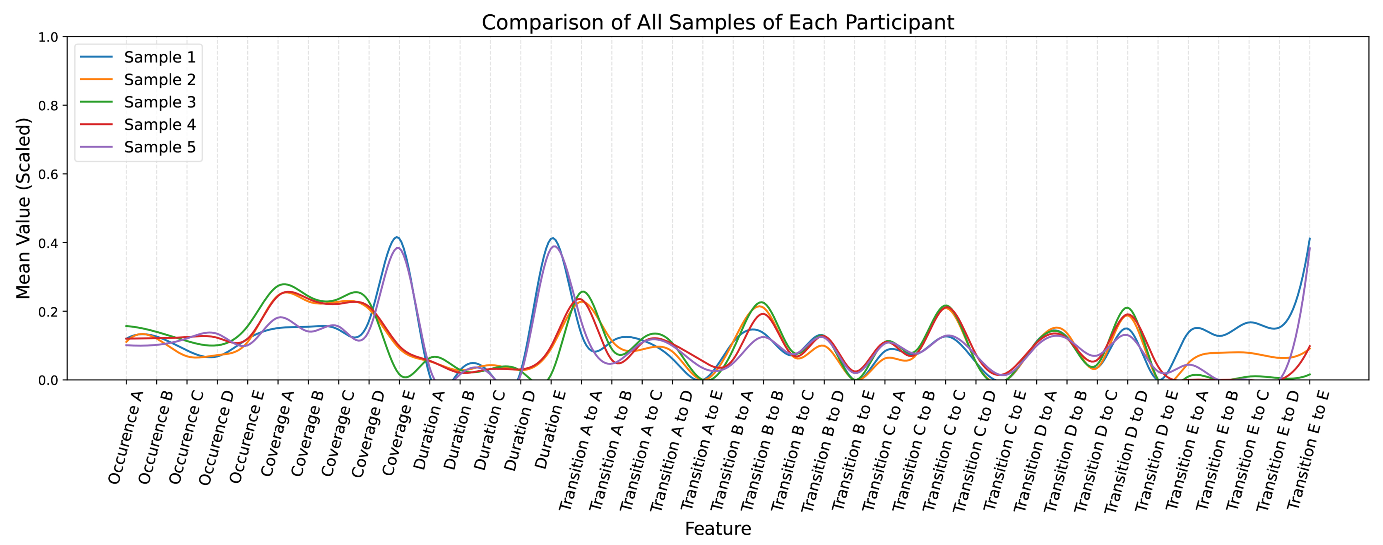
Figure 4. Comparison of feature distributions across all samples grouped by participant (intra-subject variability).
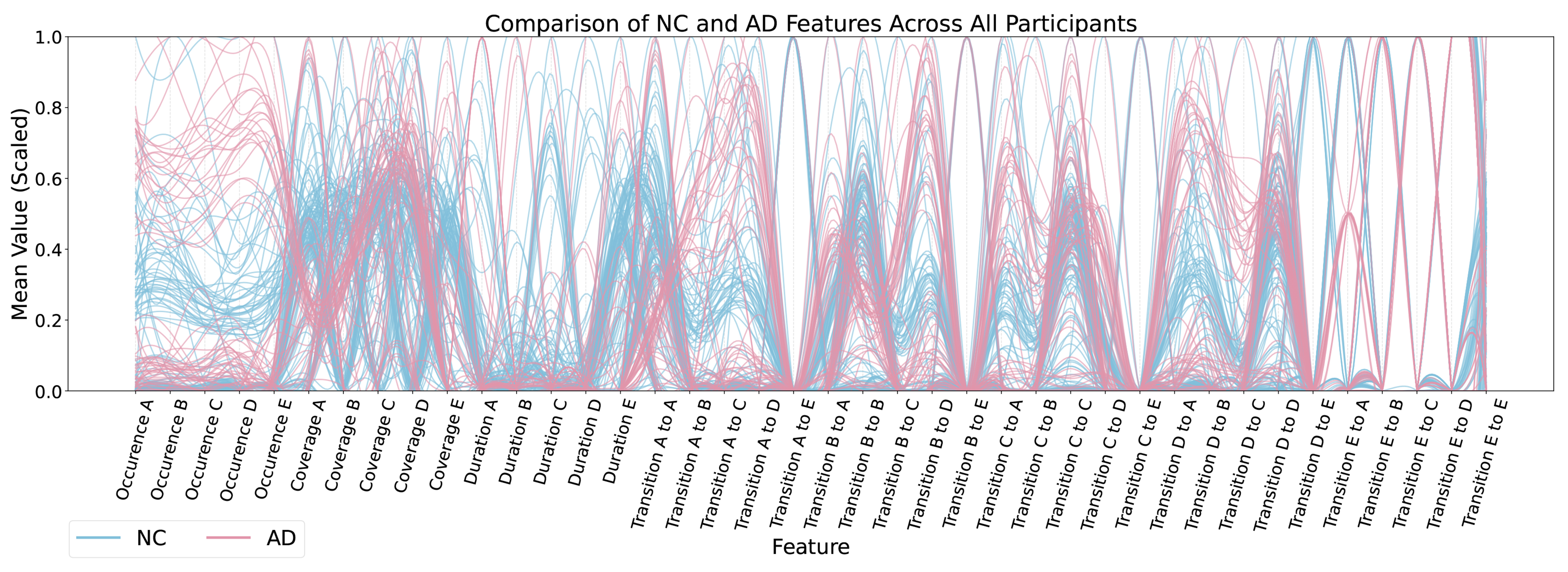
Figure 5. Comparison of feature distributions between NC and AD participants (inter-group variability). NC: Normal control; AD: Alzheimer’s disease.
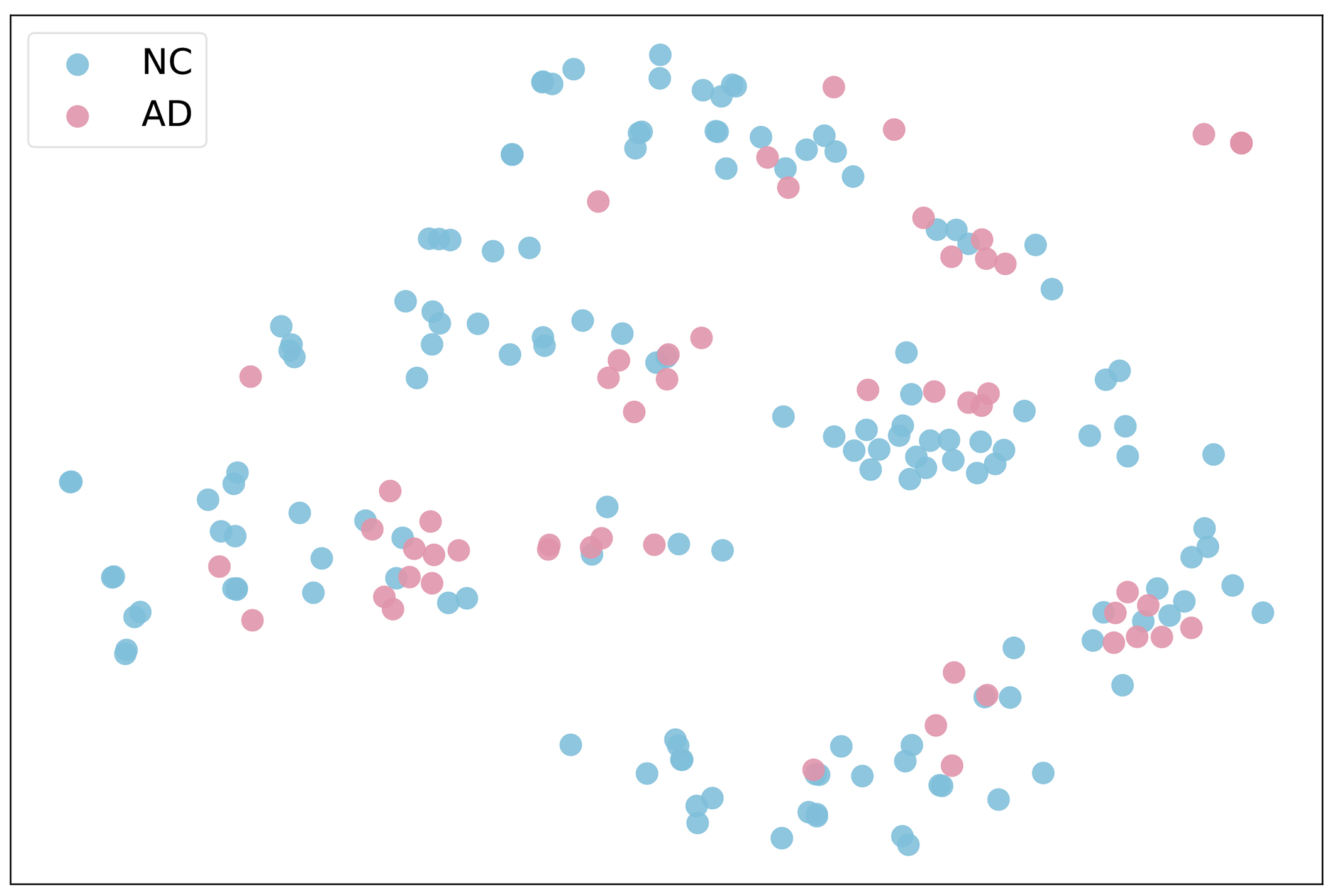
Figure 6. t-SNE projection of NC and AD samples by participant ID, illustrating feature-level clustering by group. t-SNE: t-Distributed stochastic neighbour embedding; NC: normal control; AD: Alzheimer’s disease.
7. LIMITATIONS
First, the repeated-sample cross-validation protocol adopted in this study reflects a closed-set evaluation scenario in which participants may appear in both the training and testing partitions across different folds. This design aligns with the study objective of assessing robustness to session variability; however, it should not be interpreted as a subject-independent evaluation. Excluding test participants entirely from the training set would transform the problem into an open-set biometric verification task, requiring alternative modelling strategies, such as metric-learning frameworks, Siamese architectures, or threshold-based rejection mechanisms, together with evaluation metrics centred on EER rather than classification accuracy. A leave-one-dataset-out protocol could provide a more stringent assessment of cross-device and cross-cohort generalisation. Nevertheless, the relatively small sample sizes of several constituent datasets (e.g., n = 19 for CHBMP) limit the statistical stability of such evaluations without access to additional data. Similarly, dataset-specific and channel-configuration-specific analyses were not conducted owing to limited sample availability. Future work will investigate stratified evaluations with bootstrapped confidence intervals, with particular attention to the impact of channel density (19, 64, and 128 channels) on biometric performance.
From a methodological perspective, the ablation study presented in Table 4 demonstrates the importance of the stacked ensemble strategy but does not fully disentangle the contribution of individual architectural components. Additional experiments comparing microstate-derived features with conventional EEG representations, such as spectral band-power features, would provide further insight into the discriminative value of the proposed feature space. Likewise, evaluating the MHA, 1D-CNN, and ESN modules independently against the complete EchoMC architecture would clarify the contribution of each design choice. These analyses are planned for future investigation.
Furthermore, the current implementation of EchoMC applies the ESN to the aggregated 40-dimensional microstate feature representation rather than to the original microstate symbolic sequence comprising approximately 12,000 samples. Although this configuration yielded favourable empirical results and benefits from the reservoir’s non-linear projection properties, it does not fully exploit the temporal modelling capabilities typically associated with reservoir computing. Direct processing of the microstate sequence by the ESN, together with a systematic comparison against the current feature-level formulation, represents a natural extension of the present work.
The fairness analysis relies on OAE and ΔECE, both established metrics in the broader algorithmic fairness literature. However, biometric systems are more commonly assessed using group-specific FAR, FRR, and EER measures, particularly in verification settings where threshold selection is critical. Future work will therefore incorporate these biometric fairness metrics and report confidence intervals to complement the split-level standard deviations presented in this study.
Finally, several practical considerations may limit near-term deployment. Conventional wet-electrode EEG acquisition typically requires trained personnel, preparation times ranging from approximately 20 to 45 min, and a period of sustained user cooperation during the resting-state recording protocol. In addition, clinical-grade EEG systems with 19-128 channels remain costly and are not widely accessible outside specialised environments. For individuals with AD, these limitations may be partially mitigated by the fact that EEG equipment is routinely available within neurological care settings. In such contexts, Bio-MEEG may be considered as a potential password-free authentication mechanism for accessing electronic medical records. Broader deployment beyond clinical environments would require validation on portable and dry-electrode EEG system[73], which are more suitable for daily use. Although the proposed microstate-based framework can, in principle, be applied across different EEG montages, its robustness to variations in channel count and hardware configuration remains to be established empirically.
8. CONCLUSIONS
Bio-MEEG was developed to address several limitations commonly observed in the EEG-based authentication literature, including limited cross-dataset evaluation, variation in EEG acquisition configurations, and the relatively infrequent consideration of algorithmic fairness. The proposed framework combines EEG microstate analysis with the EchoMC stacking ensemble, comprising MHA, 1D-CNN, and ESN base learners and a RF meta-classifier. Evaluation was conducted on 203 participants, including both cognitively NC individuals and individuals with AD, drawn from four datasets acquired using 19-, 64-, and 128-channel EEG systems.
Among the meta-models examined, RF was the only approach that consistently satisfied the predefined ΔECE fairness criterion across all eight demographic subgroup comparisons while maintaining competitive classification performance. In addition, the statistical analyses indicate that the extracted microstate features contain subject-discriminative information and exhibit a degree of within-subject consistency across recording sessions, supporting their suitability for biometric modelling.
The inclusion of participants with AD extends evaluation beyond the populations typically considered in EEG-based authentication studies. Given the challenges that cognitive impairment may pose for conventional credential-based authentication, this population represents a potentially relevant application context. The present results suggest that microstate-based EEG biometrics warrant further investigation in this setting; however, the findings should be interpreted within the constraints of the current experimental design. Practical deployment would require validation on portable and dry-electrode EEG systems, as well as assessment under real-world operating conditions involving users with AD.
DECLARATIONS
Authors’ contributions
Made substantial contributions to conception and design of the study and performed data analysis and interpretation: Nguyen, Q. T.; Zhang, C.
Performed data acquisition, as well as provided administrative, technical, and material support: Le, L.; King, D. W.; Vo, L.; Murris, J.; Zhang, S.; Trung, N. D.
Availability of data and materials
This study analysed four publicly available EEG datasets, all of which are accessible from their original repositories: the CHBMP dataset[44] (https://portal.conp.ca/dataset?id=projects/CHBMP), the DS004504 dataset[45] (https://openneuro.org/datasets/ds004504/versions/1.0.9), the BrainLat dataset[46] (https://www.synapse.org/Synapse:syn51549340/wiki/624187), and the PEARL-Neuro Database[47] (https://openneuro.org/datasets/ds004796/versions/1.1.0). No new data were generated in this study. The processed feature matrices and source code used to reproduce the experiments are available from the corresponding author upon reasonable request.
AI and AI-assisted tools statement
During the preparation of this manuscript, the AI tools ChatGPT (version 4o), Claude (version Sonnet 4.5), and Gemini (version 2.0 Flash) were used solely for language editing. The tools did not influence the study design, data collection, analysis, interpretation, or the scientific content of the work. All authors take full responsibility for the accuracy, integrity, and final content of the manuscript.
Financial support and sponsorship
None.
Conflicts of interest
All authors declare that they are bound by confidentiality agreements that prevent them from disclosing their conflicts of interest in this work.
Ethical approval and consent to participate
Not applicable.
Consent for publication
Not applicable.
Copyright
The Author(s) 2026.
REFERENCES
1. Lassak, L.; Markert, P.; Golla, M.; Stobert, E.; Dürmuth, M. A comparative long-term study of fallback authentication schemes. In Proceedings of the 2024 CHI Conference on Human Factors in Computing Systems. Association for Computing Machinery: 2024; pp. 1-19.
2. Constantinides, A.; Belk, M.; Fidas, C.; et al. Security and usability of a personalized user authentication paradigm: insights from a longitudinal study with three healthcare organizations. ACM. Trans. Comput. Healthc. 2023, 4, 1-40.
3. He, H.; Liao, R.; Li, Y. MSAFNet: a novel approach to facial expression recognition in embodied AI systems. Intell. Robot. 2025, 5, 313-32.
4. Nakamura, T.; Goverdovsky, V.; Mandic, D. P. In-ear EEG biometrics for feasible and readily collectable real-world person authentication. IEEE. Trans. Inf. Forensics. Secur. 2018, 13, 648-61.
5. Aldayel, M.; Alsedairy, N.; Al-Nafjan, A.; Alsenan, S. Systematic review of brain-computer interface based user authentication system: trends, challenges, and directions. IEEE. Access. 2024, 12, 96848-61.
6. Seyfizadeh, A.; Peach, R. L.; Tovote, P.; Isaias, I. U.; Volkmann, J.; Muthuraman, M. Enhancing security in brain–computer interface applications with deep learning: electroencephalogram-based user identification. Expert. Syst. Appl. 2024, 253, 124218.
7. Colafiglio, T.; Lofù, D.; Sorino, P.; et al. EmoSynth real time emotion-driven sound texture synthesis via brain-computer interface. In Adjunct Proceedings of the 32nd ACM Conference on User Modeling, Adaptation and Personalization (UMAP). Association for Computing Machinery: 2024; pp. 616-21.
8. Białas, K.; Kedziora, M.; Chałupnik, R.; Song, H. H. Multifactor authentication system using simplified EEG brain–computer interface. IEEE. Trans. Hum. Mach. Syst. 2022, 52, 867-76.
9. Peng, Y.; Jiang, Y.; Zuo, Z.; Gu, S.; Wang, Z.; Tian, Z. A rehabilitation design concept based on brain–computer interface and McKibben artificial muscle. Healthc. Rehabil. 2026, 2, 100066.
10. Bidgoly, A. J.; Bidgoly, H. J.; Arezoumand, Z. A survey on methods and challenges in EEG based authentication. Comput. Secur. 2020, 93, 101788.
11. Jin, J.; Chen, Z.; Cai, H.; Pan, J. Affective EEG-based person identification with continual learning. IEEE. Trans. Instrum. Meas. 2024, 73, 1-16.
12. Chaurasia, A. K.; Fallahi, M.; Strufe, T.; Terhörst, P.; Cabarcos, P. A. NeuroIDBench: an open-source benchmark framework for the standardization of methodology in brainwave-based authentication research. J. Inf. Secur. Appl. 2024, 85, 103832.
13. Nguyen, Q. T.; Le, L.; Williams-King, D.; Tang, Q. H.; Duong-Trung, N. Explainable AI for dementia detection using EEG microstates. In Companion Proceedings of the 31st International Conference on Intelligent User Interfaces. Association for Computing Machinery: 2026; pp. 39-42.
14. Adebisi, A. T.; Lee, H. W.; Veluvolu, K. C. EEG-based brain functional network analysis for differential identification of dementia-related disorders and their onset. IEEE. Trans. Neural. Syst. Rehabil. Eng. 2024, 32, 1198-209.
15. Hogges, J.; Shahriar, H.; Sneha, S.; Ahamed, S. A two-step password authentication system for Alzheimer patients. In 2020 IEEE 44th Annual Computers, Software, and Applications Conference (COMPSAC), Madrid, Spain, July 13-17, 2020. IEEE: 2020; pp. 1444-8.
16. Raivio, M. M.; Mäki-Petäjä-Leinonen, A. P.; Laakkonen, M. L.; Tilvis, R. S.; Pitkälä, K. H. The use of legal guardians and financial powers of attorney among home-dwellers with Alzheimer’s disease living with their spousal caregivers. J. Med. Ethics. 2008, 34, 882-6.
17. Gaikwad, S.; Senapati, S.; Haque, M. A.; Kayed, R. Senescence, brain inflammation, and oligomeric tau drive cognitive decline in Alzheimer’s disease: evidence from clinical and preclinical studies. Alzheimers. Dement. 2024, 20, 709-27.
18. Hughes, J.; Pastrana, S.; Hutchings, A.; et al. The art of cybercrime community research. ACM. Comput. Surv. 2024, 56, 1-26.
19. Lassi, M.; Fabbiani, C.; Mazzeo, S.; et al. Degradation of EEG microstates patterns in subjective cognitive decline and mild cognitive impairment: early biomarkers along the Alzheimer’s disease continuum? NeuroImage. Clin. 2023, 38, 103407.
20. Huber, M.; Luu, A. T.; Boutros, F.; Kuijper, A.; Damer, N. Bias and diversity in synthetic-based face recognition. In Proceedings of the IEEE/CVF Winter Conference on Applications of Computer Vision (WACV). 2024; pp. 6215-26.
21. Drozdowski, P.; Rathgeb, C.; Dantcheva, A.; Damer, N.; Busch, C. Demographic bias in biometrics: a survey on an emerging challenge. IEEE. Trans. Technol. Soc. 2020, 1, 89-103.
22. Pappula, M.; Anwar, S. M. An ADHD diagnostic interface based on EEG spectrograms and deep learning techniques. In 2024 20th International Symposium on Medical Information Processing and Analysis (SIPAIM), Antigua, Guatemala, Nov 13-15, 2024. IEEE: 2024; p. 1-4.
23. Haider, C. M. R.; Clifton, C.; Zhou, Y. Unfair AI: it isn’t just biased data. In 2022 IEEE International Conference on Data Mining (ICDM), Orlando, USA, Nov 28 - Dec 01, 2022. IEEE: 2022; pp. 957-62.
24. Sun, J.; Sun, Y.; Shen, A.; Li, Y.; Gao, X.; Lu, B. An ensemble learning model for continuous cognition assessment based on resting-state EEG. NPJ. Aging. 2024, 10, 1.
25. Sun, C.; Song, M.; Cai, D.; Zhang, B.; Hong, S.; Li, H. A systematic review of echo state networks from design to application. IEEE. Trans. Artif. Intell. 2024, 5, 23-37.
26. Wang, Z.; Sun, J. TransTab: learning transferable tabular transformers across tables. Adv. Neural. Inf. Process. Syst. 2022, 35, 2902-15.
27. Shwartz-Ziv, R.; Armon, A. Tabular data: deep learning is not all you need. Inf. Fusion. 2022, 81, 84-90.
28. Goetz, L.; Seedat, N.; Vandersluis, R.; van der Schaar, M. Generalization - a key challenge for responsible AI in patient-facing clinical applications. NPJ. Digit. Med. 2024, 7, 126.
29. Chen, Y.; Atnafu, A. D.; Schlattner, I.; et al. A high-security EEG-based login system with RSVP stimuli and dry electrodes. IEEE. Trans. Inf. Forensics. Secur. 2016, 11, 2635-47.
30. Wu, Q.; Yan, B.; Zeng, Y.; Zhang, C.; Tong, L. Anti-deception: reliable EEG-based biometrics with real-time capability from the neural response of face rapid serial visual presentation. BioMed. Eng. OnLine. 2018, 17, 55.
31. Mu, Z.; Hu, J.; Min, J. EEG-based person authentication using a fuzzy entropy-related approach with two electrodes. Entropy 2016, 18, 432.
32. Wu, Q.; Zeng, Y.; Zhang, C.; Tong, L.; Yan, B. An EEG-based person authentication system with open-set capability combining eye blinking signals. Sensors 2018, 18, 335.
33. Thomas, K. P.; Vinod, A. P. EEG-based biometric authentication using gamma band power during rest state. Circuits. Syst. Signal. Process. 2018, 37, 277-89.
34. Kumar, P.; Saini, R.; Kaur, B.; Roy, P. P.; Scheme, E. Fusion of neuro-signals and dynamic signatures for person authentication. Sensors 2019, 19, 4641.
35. Zeynali, M.; Seyedarabi, H. EEG-based single-channel authentication systems with optimum electrode placement for different mental activities. Biomed. J. 2019, 42, 261-7.
36. Seha, S. N. A.; Hatzinakos, D. EEG-based human recognition using steady-state AEPs and subject-unique spatial filters. IEEE. Trans. Inf. Forensics. Secur. 2020, 15, 3901-10.
37. Rathi, N.; Singla, R.; Tiwari, S. A novel approach for designing authentication system using a picture based P300 speller. Cogn. Neurodyn. 2021, 15, 805-24.
38. Yap, H. Y.; Choo, Y. H.; Mohd Yusoh, Z. I.; Khoh, W. H. An evaluation of transfer learning models in EEG-based authentication. Brain. Inform. 2023, 10, 19.
39. Alsumari, W.; Hussain, M.; Alshehri, L.; Aboalsamh, H. A. EEG-based person identification and authentication using deep convolutional neural network. Axioms 2023, 12, 74.
40. Ferdi, A. Y.; Ghazli, A. Authentication with a one-dimensional CNN model using EEG-based brain-computer interface. Comput. Methods. Biomech. Biomed. Eng. 2025, 28, 1969-80.
41. Bolouri, S.; Shukla, D. An EEG-based user authentication system using event-related potentials and ensemble learning. In 2024 Cyber Awareness and Research Symposium (CARS), Grand Forks, USA, Oct 28-29, 2024. IEEE: 2024; p. 1-6.
42. Gong, Y.; Wang, M.; Zhang, Y.; Zhang, W.; Pang, S. A unified deep learning-based EEG biometric authentication system for cross-session scenarios. In International Conference on Advanced Data Mining and Applications. Springer: 2024; pp. 48-62.
43. Mishra, A. R.; Kumar, R.; Saini, R. Performance enhancement of EEG signatures for person authentication using CNN BiLSTM method. J. Univ. Comput. Sci. 2024, 30, 1755-79.
44. Valdes-Sosa, P. A.; Galan-Garcia, L.; Bosch-Bayard, J.; et al. The Cuban Human Brain Mapping Project, a young and middle age population-based EEG, MRI, and cognition dataset. Sci. Data. 2021, 8, 45.
45. Miltiadous, A.; Tzimourta, K. D.; Afrantou, T.; et al. A dataset of scalp EEG recordings of Alzheimer’s disease, frontotemporal dementia and healthy subjects from routine EEG. Data 2023, 8, 95.
46. Prado, P.; Medel, V.; Gonzalez-Gomez, R.; et al. The BrainLat project, a multimodal neuroimaging dataset of neurodegeneration from underrepresented backgrounds. Sci. Data. 2023, 10, 889.
47. Dzianok, P.; Kublik, E. PEARL-Neuro Database: EEG, fMRI, health and lifestyle data of middle-aged people at risk of dementia. Sci. Data. 2024, 11, 276.
48. Chu, C.; Zhang, Z.; Song, Z.; et al. An enhanced EEG microstate recognition framework based on deep neural networks: an application to Parkinson’s disease. IEEE. J. Biomed. Health. Inform. 2023, 27, 1307-18.
49. Antonova, E.; Holding, M.; Suen, H. C.; Sumich, A.; Maex, R.; Nehaniv, C. EEG microstates: functional significance and short-term test-retest reliability. Neuroimage. Rep. 2022, 2, 100089.
50. Nguyen, Q. T. Standardising number of EEG sensors for AI-driven dementia detection. IEEE. Sens. Lett. 2025, 9, 1-4.
51. Nguyen, Q. T.; Le, L.; Tran, X. T. et. al. Transforming brainwaves into language: EEG microstates meet text embedding models for dementia detection. In The 63rd Annual Meeting of the Association for Computational Linguistics, Vienna, Austria. Association for Computational Linguistics: 2025; pp. 186-202.
52. Tarailis, P.; Koenig, T.; Michel, C. M.; Griškova-Bulanova, I. The functional aspects of resting EEG microstates: a systematic review. Brain. Topogr. 2024, 37, 181-217.
53. Khanna, A.; Pascual-Leone, A.; Farzan, F. Reliability of resting-state microstate features in electroencephalography. PloS. One. 2014, 9, e114163.
54. Koenig, T.; Kottlow, M.; Stein, M.; Melie-García, L. Ragu: a free tool for the analysis of EEG and MEG event-related scalp field data using global randomization statistics. Comput. Intell. Neurosci. 2011, 2011, 938925.
55. Pascual-Marqui, R. D.; Michel, C. M.; Lehmann, D. Segmentation of brain electrical activity into microstates: model estimation and validation. IEEE. Trans. Biomed. Eng. 1995, 42, 658-65.
56. Bagdasarov, A.; Roberts, K.; Bréchet, L.; Brunet, D.; Michel, C. M.; Gaffrey, M. S. Spatiotemporal dynamics of EEG microstates in four-to eight-year-old children: age-and sex-related effects. Dev. Cogn. Neurosci. 2022, 57, 101134.
57. Valt, C.; Tavella, A.; Berchio, C.; et al. MEG microstates: an investigation of underlying brain sources and potential neurophysiological processes. Brain. Topogr. 2024, 37, 993-1009.
58. Zhao, X.; Li, Z.; Zhao, C.; Fu, R.; Wang, C. Distraction-level recognition based on stacking ensemble learning for IVIS secondary tasks. Expert. Syst. Appl. 2024, 244, 122849.
59. Vaswani, A.; Shazeer, N.; Parmar, N.; et al. Attention is all you need. In Advances in Neural Information Processing Systems 30: Annual Conference on Neural Information Processing Systems 2017, Long Beach, USA, Dec 4-9, 2017. 2017; pp. 5998-6008. https://proceedings.neurips.cc/paper/2017/hash/3f5ee243547dee91fbd053c1c4a845aa-Abstract.html. (accessed 2026-06-25).
61. Yan, M.; Huang, C.; Bienstman, P.; Tino, P.; Lin, W.; Sun, J. Emerging opportunities and challenges for the future of reservoir computing. Nat. Commun. 2024, 15, 2056.
62. Wootton, A. J.; Taylor, S. L.; Day, C. R.; Haycock, P. W. Optimizing echo state networks for static pattern recognition. Cogn. Comput. 2017, 9, 391-9.
63. Amin, E.; Elgammal, Y. M.; Zahran, M. A.; Abdelsalam, M. M. Alzheimer’s disease: new insight in assessing of amyloid plaques morphologies using multifractal geometry based on Naive Bayes optimized by random forest algorithm. Sci. Rep. 2023, 13, 18568.
64. Yuan, Y.; Wang, W.; Guo, Q.; Xiong, Y.; Shen, C.; He, P. Does ChatGPT know that it does not know? Evaluating the black-box calibration of ChatGPT. In Proceedings of the 2024 Joint International Conference on Computational Linguistics, Language Resources and Evaluation (LREC-COLING 2024). ELRA and ICCL: 2024; pp. 5191-201. https://aclanthology.org/2024.lrec-main.462/. (accessed 2026-06-25).
66. Pessach, D.; Shmueli, E. A review on fairness in machine learning. ACM. Comput. Surv. 2022, 55, 1-44.
67. Férat, V.; Scheltienne, M.; Brunet, D.; Ros, T.; Michel, C. Pycrostates: a Python library to study EEG microstates. J. Open. Source. Softw. 2022, 7, 4564.
68. Fisher, R. A. Statistical methods for research workers. 1934. https://archive.org/details/in.ernet.dli.2015.205971. (accessed 2026-06-25).
69. Stouffer, S. A.; Suchman, E. A.; DeVinney, L. C.; Star, S. A.; Williams, R. M. The American soldier: adjustment during army life. 1949. https://gwern.net/doc/psychology/1949-stouffer-theamericansoldier-v1-adjustmentduringarmylife.pdf. (accessed 2026-06-25).
70. Goeman, J. J.; Solari, A. Multiple hypothesis testing in genomics. Stat. Med. 2014, 33, 1946-78.
73. Nguyen, Q. T.; Huiru, Z.; Tazin, T.; et al. Emotion recognition using text embedding models: wearable and wireless EEG without fixed EEG channel configurations. In Adjunct Proceedings of the 33rd ACM Conference on User Modeling, Adaptation and Personalization. Association for Computing Machinery: 2025; pp. 476-88.
74. Zeng, Y.; Wu, Q.; Yang, K.; et al. EEG-based identity authentication framework using face rapid serial visual presentation with optimized channels. Sensors 2018, 19, 6.
75. Ortega-Rodríguez, J.; Gómez-González, J. F.; Pereda, E. Selection of the minimum number of EEG sensors to guarantee biometric identification of individuals. Sensors 2023, 23, 4239.
76. Gorur, K.; Olmez, E.; Ozer, Z.; Cetin, O. EEG-driven biometric authentication for investigation of fourier synchrosqueezed transform-ICA robust framework. Arab. J. Sci. Eng. 2023, 48, 10901-23.
Cite This Article
How to Cite
Download Citation
Export Citation File:
Type of Import
Tips on Downloading Citation
Citation Manager File Format
Type of Import
Direct Import: When the Direct Import option is selected (the default state), a dialogue box will give you the option to Save or Open the downloaded citation data. Choosing Open will either launch your citation manager or give you a choice of applications with which to use the metadata. The Save option saves the file locally for later use.
Indirect Import: When the Indirect Import option is selected, the metadata is displayed and may be copied and pasted as needed.
About This Article
Copyright

Data & Comments
Data
0


Comments
Comments must be written in English. Spam, offensive content, impersonation, and private information will not be permitted. If any comment is reported and identified as inappropriate content by OAE staff, the comment will be removed without notice. If you have any queries or need any help, please contact us at [email protected].