Learning-based cooperative decision-making and control for multiple autonomous vehicles in unsignalized intersections
Abstract
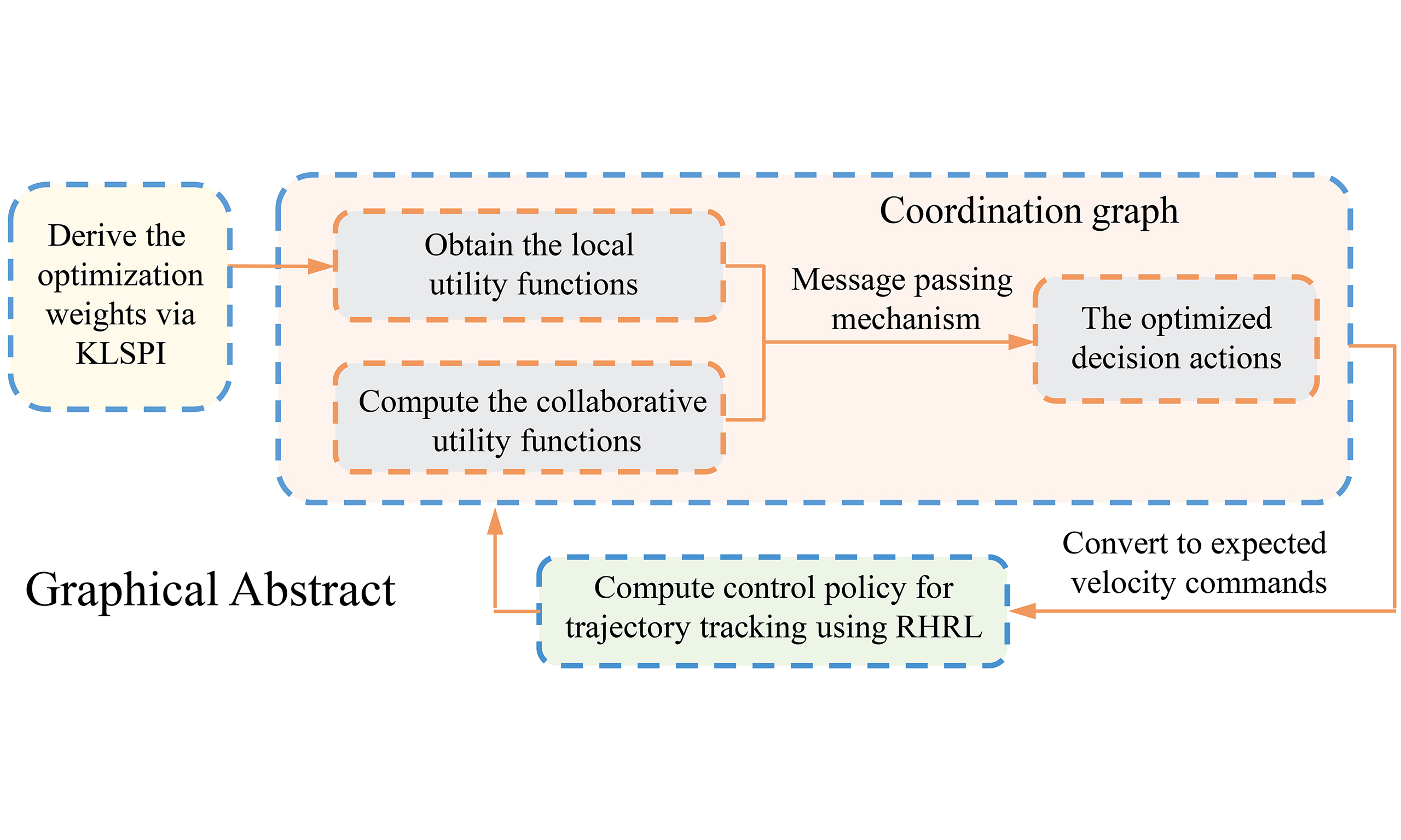
Cooperative navigation of multiple autonomous vehicles (MAVs) at unsignalized intersections remains a core challenge in intelligent transportation systems. This paper proposes a learning-based cooperative decision-making and control (LCDMC) method for MAVs, which improves policy learning efficiency and ensures safe and efficient cooperative navigation. In the proposed LCDMC algorithm, the global value function is decomposed into two components: a local utility function and a joint-action utility function among vehicles, which incorporates both the offline policy learning phase and the online deployment phase. During the offline phase, the kernel-based least-squares policy iteration method is employed to learn localized decision-making policies from high-dimensional samples. In the online deployment phase, a coordination graph for MAVs is developed, and a collaborative utility function characterizing joint action performance is designed. To solve optimized decision actions, the local utility function is integrated with a message propagation mechanism, and then the decision actions are converted into velocity commands. Furthermore, a receding-horizon reinforcement learning approach is designed to achieve trajectory tracking control of the autonomous vehicles in MAVs. Finally, to verify the effectiveness of the proposed method, numerical simulations of MAVs are performed, and the results demonstrate that the proposed LCDMC method exhibits superior performance in both traffic efficiency and safety for cooperative navigation of MAVs at unsignalized intersections.
Keywords
1. INTRODUCTION
Autonomous driving technology is advancing at an unprecedented pace and demonstrating significant application potential in real-world traffic scenarios[1,2]. Although autonomous vehicles (AVs) perform well in structured environments such as highways, their deployment in urban road settings still faces numerous challenges. Urban road environments are intricate and complex, containing a multitude of uncertainties. This uncertainty significantly increases the difficulty of decision-making for AVs[3]. Among these challenges, one of the most demanding scenarios is the unsignalized urban intersection. Relevant research indicates that even experienced human drivers often experience considerable pressure at such intersections, where momentary lapses can potentially lead to traffic accidents[4]. Therefore, enhancing the capability of autonomous driving systems to respond effectively in such high-risk scenarios is a critical research direction.
The cooperative navigation of multiple vehicles in unsignalized intersections poses key challenges, including high-dimensional nonlinear dynamics, incomplete-information Nash equilibrium, and uncertainty in neighboring vehicle behaviors, thus attracting extensive research attention[5,6]. In recent years, the cooperative navigation problem between AVs and multiple human-driven vehicles at intersection scenarios has been widely investigated, primarily focusing on AVs decision-making mechanisms[7,8], path planning[9], and social behavior modeling[10]. However, the aforementioned methods are inadequate for fully autonomous and cooperative intersection scenarios, which require further research on distributed negotiation mechanisms, multi-agent collaborative decision-making frameworks, and global traffic efficiency optimization strategies. Cooperative decision-making and control schemes for multi-vehicle systems have demonstrated potential to enhance traffic throughput efficiency and safety[11,12], particularly under dynamic and uncertain environments. The common coordination methods for multi-vehicle systems can be systematically categorized into the following classes: rule-based decision-making approaches, convex optimization-based methods[13], game-theoretic models[14,15], and learning-based decision-making frameworks[16].
Rule-based decision-making methods involve creating a rule database for vehicle behaviors in operational scenarios based on experience and predefined rules. These rules enable a deterministic mapping from vehicle states to behaviors, with typical approaches such as finite state machine (FSM)[17], first come first served (FCFS)[18], and longest queue first (LQF)[19]. Rule-based methods exhibit clear logic, operational stability, and strong practicality. However, their finite state representation may inadequately capture all operational conditions faced by AVs, and limited scenario coverage degrades decision-making performance in complex dynamic environments. Furthermore, Liu et al. designed a multi-agent game-theoretic attention-based deep deterministic policy gradient algorithm[20], which improves traffic flow efficiency at unsignalized intersections. Although game-theoretic methods offer theoretical advantages for multi-agent intersection coordination, they face scalability issues due to computational inefficiency and reduced accuracy in modeling vehicle dynamics in complex traffic scenarios.
Learning-based decision-making methods primarily include Bayesian inference[21,22], decision trees[23], and Markov decision processes[24]. In multi-agent systems, reinforcement learning (RL), particularly deep reinforcement learning (DRL), has become the primary approach for solving complex sequential decision-making problems [25]. Current research in multi-agent deep reinforcement learning (MDRL) is rapidly expanding into real-world traffic scenarios. The focus has shifted from fundamental tasks such as lane changing[26–28] and overtaking[29,30] to more complex collaborative decision-making on road systems. Chen et al. developed a curriculum learning-based decision-making framework for highway on-ramp merging to improve traffic flow efficiency and safety under mixed traffic conditions[31]. Guo et al. proposed a heuristic MDRL algorithm by combining the advantages of heuristic strategies and deep learning[32], which enhances the smoothness and safety of traffic flow at intersections. Zhao et al. presented a safety RL method based on multi-agent projection-constrained policy optimization [33], demonstrating superior coordination performance for AVs at unsignalized intersections. However, although the aforementioned methods have achieved considerable performance, they generally suffer from high algorithmic complexity and computational costs. Moreover, most of these methods are designed for specific scenarios and rely on idealized assumptions, which significantly limit their practicality. Additionally, non-stationarity and poor interpretability also make these methods difficult to apply in real-world scenarios. To tackle the issues of excessive parameter size and slow inference speed in AV decision-making models, a lightweight optimization approach based on Video Swin Transformer and DRL is proposed in Ref[34]. This method effectively reduced model parameters and memory requirements while improving inference efficiency for long-sequence tasks through parallel spatiotemporal feature extraction with risk assessment mechanisms and the adoption of double-softmax linear self-attention. However, this approach still exhibits limitations including difficulties in hyperparameter tuning and performance degradation on short-sequence tasks.
To address the above problem, the paper proposes a learning-based cooperative decision-making and control (LCDMC) method for multiple AVs (MAVs), improving policy learning efficiency while ensuring safe and efficient cooperative navigation. The LCDMC method decomposes the global value function of the system into two components: a local utility function and a collaborative utility function representing the joint actions among vehicles, thereby enhancing the representational capacity of value functions in multi-agent RL. Numerical simulations of MAVs demonstrate that the LCDMC method exhibits superior performance in both traffic efficiency and safety for cooperative navigation of MAVs at unsignalized intersections. The main contributions are listed as follows.
The subsequent sections of the paper are structured as follows. Section 2 analyzes the foundational concepts of Markov decision process modeling for MAVs and coordination graphs. In Section 3, a LCDMC approach for MAVs is proposed. Section 4 carries out simulation verification, while Section 5 draws conclusions.
2. PRELIMINARIES AND PROBLEM FORMULATION
2.1. MAVs Markov decision process modeling
The MAVs' cooperative decision-making at intersections is modeled as a decentralized partially observable Markov decision process (Dec-POMDP), which is given by the following tuple:
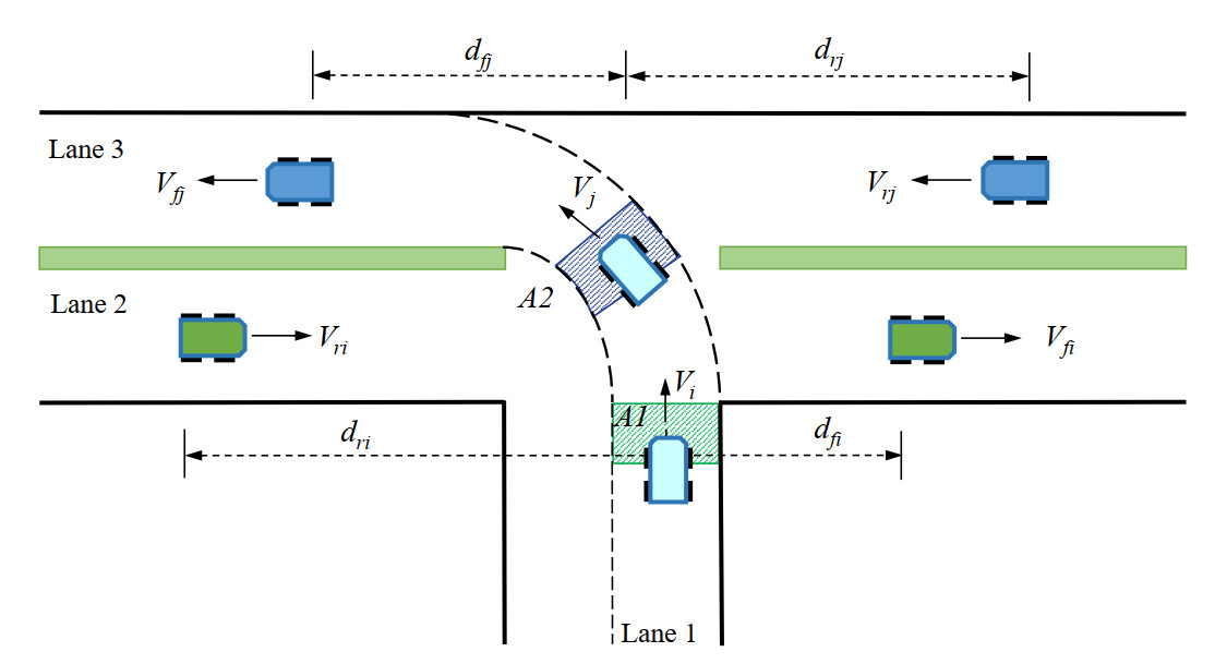
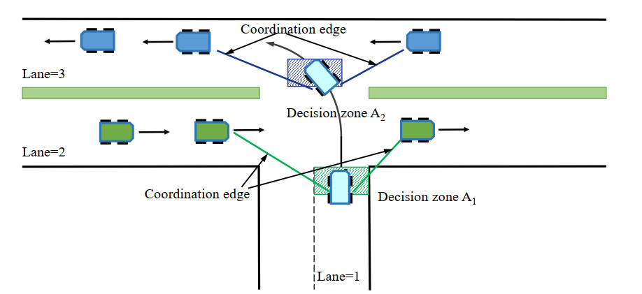
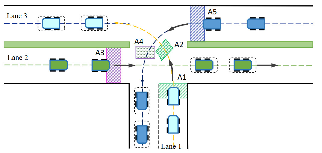
As shown in Figure 1, a T-junction without traffic signals involves six AVs requiring cooperative decision-making, including left-turning vehicles, right-going straight vehicles, and left-going straight vehicles. The state space of the
2.2. Coordination graphs
Probabilistic graphical model (PGM) integrates probability theory with graph theory and constitutes a pivotal research direction in machine learning[36]. PGM primarily focuses on the representation, inference, and learning of directed graphical models and undirected graphical models. A core objective in artificial intelligence is to extract implicit, fundamental knowledge from observed data, and PGM serves as a powerful methodology to achieve this goal. In MAVs systems, nodes of the probabilistic graph represent vehicles, while edges with connecting relationships describe the local performance of joint actions taken by adjacent vehicles, inferring the posterior distribution of joint actions based on current vehicle information. Probabilistic graph-based approaches can effectively model coupling relationships among MAVs, which facilitate the construction of large-scale artificial intelligence systems to address complex real-world problems.
The coordinated RL method introduces a coordination graph to establish connecting edges among agents with cooperative relationships[37]. The messages
where
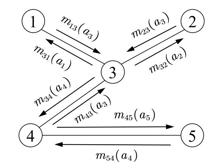
The Ref[36] demonstrates a direct duality between computing the maximum posteriori probability in PGM and solving the optimal joint action in coordination graphs. Consequently, the belief propagation algorithm, used for inference in PGM, is also applicable to multi-agent collaborative decision-making using coordination graphs. In Figure 2, agent
where
which indicates that the state-action value function of agent
Building upon the aforementioned mechanism, this paper proposes a LCDMC method for MAVs. The local utility function
3. LCDMC FOR MAVS
This section presents the LCDMC method for MAVs. The method employs KLSPI to solve the local utility function and integrates a message-passing mechanism via a cooperation graph to compute the optimized decision actions for AVs, which are then used as reference signals. Furthermore, a receding-horizon RL (RHRL) method is designed for trajectory tracking control of AVs.
3.1. The overall framework of the proposed method
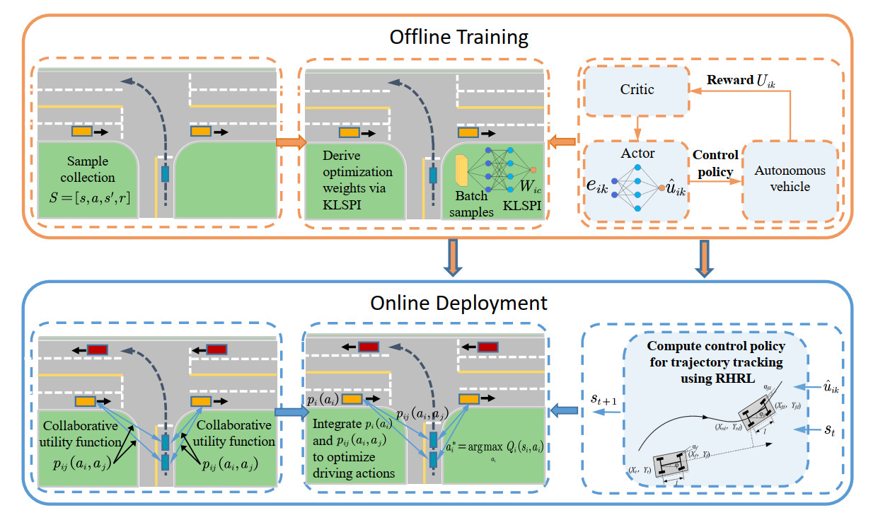
The proposed algorithm primarily consists of two stages: offline policy learning and online deployment implementation. The algorithmic framework is depicted in Figure 3. In the offline training phase, samples are collected using a random policy. An approximate linear dependency (ALD) analysis is employed to learn model features and construct the kernel dictionary from the high-dimensional state space, thereby reducing the dimensionality of the samples. Then, a sparse kernel-based least-squares RL method is adopted to learn the policy. During the online deployment phase, when AV
Figure 3. The block diagram of the proposed LCDMC algorithm. LCDMC: Learning-based cooperative decision-making and control.
Based on coordination graph theory, the global state-action value function is given by Equation (2). This formulation demonstrates that optimal decisions for MAVs can be computed in a distributed manner by iteratively exchanging messages along the coordination graph edges, thus avoiding exhaustive searches over the joint-action space. The proposed method contrasts with AV
3.2. Kernel-based efficient learning for local utility function
This section elaborates on the proposed LCDMC method for MAVs, which learns the local utility function via KLSPI. During the offline phase, extensive samples are pre-collected at unsignalized intersections. An optimized local decision-making policy is derived in a data-driven manner and subsequently deployed online for real-time decision-making.
In the coordinated traversal of multiple vehicles at the unsignalized intersection shown in Figure 1, the tuple for multi-vehicle cooperative decision-making modeling is defined in Equation (1). Under the current state
Sampling parameters of MAVs corresponding to the scenario displayed in Figure 1
| Lane of autonomous | Decision | Action | Front/rear vehicle | Front/rear vehicle | Front/rear vehicle |
| The scenario depicts an unsignalized T-junction where six AVs require cooperative decision-making, including left-turning vehicles in Lane 1, right-going vehicles in Lane 2, and left-going vehicles in Lane 3. MAVs: Multiple autonomous vehicles; AVs: autonomous vehicles. | |||||
| vehicles | zone (m) | space | lane | speed (m/s) | distance (m) |
| Lane 1 | {sd, kv, acc} | Lane 2 | [1,15] | [0, 50] | |
| Lane 2 | {sd, kv, acc} | Lane 1 | [1,15] | [0, 30] | |
| Lane 3 | {sd, kv, acc} | Lane 1 | [1,15] | [0, 30] | |
Upon acquiring a substantial set of samples, the KLSPI algorithm is employed for policy learning. This section extends sparse kernel-based feature representation methods[39] to cooperative decision-making in MAVs. In the proposed LCDMC framework, the local utility function of the AV is represented via basis functions constructed from feature vectors. A kernel sparsification technique is applied to extract features from the high-dimensional samples, yielding representative subsamples through ALD analysis. Assuming the kernel function
where
Then, the representative subsample is obtained using the ALD analysis technique. Sample sparsification is implemented via ALD in two steps. Firstly, the distance between sample
where
The feature construction module utilizes the subsampled points generated previously to construct the basis function for each original sample as
where
By combining Equation (9) and rewriting TD error, we have:
By multiplying both sides of Equation (10) by
where
Based on the above analysis, the KLSPI method is employed to learn local policies for AVs from collected high-dimensional samples. This method enables real-time derivation of the local utility function
3.3. Online decision-making using coordination graphs
In the proposed LCDMC method for MAVs, a cooperative relationship is established among vehicles across different lanes. The Max-plus message passing mechanism is utilized to iteratively propagate local joint-action rewards through cooperative communication edges, enabling optimized decision-making for MAVs.
The cooperative interactions among AVs are inherently dynamic due to the multi-vehicle traffic flow dynamics. At unsignalized intersections, an undirected edge between AVs
where
After AV
where
where
The term
The computational complexity of the coordination graph primarily stems from two components: coordination edge updates and message propagation. Coordination edge updates refer to the distance computation between vehicles during each path intersection detection, while message propagation denotes the iterative process of the Max-plus algorithm along each edge until convergence. The complexity is
The forming and dissolving of edges in the coordination graph are primarily determined by the vehicles' traversal tasks and spatial correlations. The specific rules are as follows. Edge forming triggered by paths intersect: each lane at an intersection has a designated decision zone. When a vehicle enters this zone, its onboard sensors detect the speed and position of leading and following vehicles in adjacent lanes. If the detected vehicles' trajectories spatially intersect, a coordination edge is established, indicating the need for cooperative decision-making. Edge dissolving triggered by complete traversal or distance threshold: the system removes the corresponding coordination edge when an AV either completes cooperative traversal or exits the decision zone, thereby reducing computational complexity.
3.4. RHRL controller for real-time trajectory tracking
A RHRL approach is designed to achieve trajectory tracking control of the AVs in this section, with the reference velocity profile determined through multi-vehicle cooperative decision-making. The kinematic model of an Ackermann-steering AV is given as
where
By combining Equations (16) and (17), the tracking error dynamics can be discretized as follows:
where
where
At the sampling instant
The costate of the value function is defined as
Then, the optimal control output is defined as
Due to the difficulty in obtaining analytical expressions of the control input for nonlinear systems, an actor-critic RL framework is adopted to learn the policy within the prediction horizon. This framework utilizes a value iteration approach, in which neural networks are employed to approximate the costate function and the optimal control input. The structure of the critic network is expressed as:
where
The critic network approximates the optimal costate by minimizing the error function
where
The actor network of the AV is a three-layer neural network that takes the tracking error
where
where
Employing the RHRL approach, an optimized control sequence is learned within the prediction horizon at time step
The online learning computational complexity of the RHRL approach stems from Equations (25) and (27), which is approximately
Based on the above analysis, the offline learning phase of the proposed method employs KLSPI to learn local policies from high-dimensional collected samples, which improve the computational efficiency and policy convergence. During the online deployment phase, when AV
Algorithm 1 The LCDMC Algorithm Require: maximum simulation step Ensure: Decision action Offline Phase 1: // Collect samples 2: for 3: Randomly initialize the vehicle's distance within the range 4: Randomly select an action 5: Determine the reward 6: end for // Train policy 7: Extract the sample features using Equation (7); 8: for 9: Construct the approximation structure of the local utility function via Equation (9); 10: Update the policy 11: if 12: 13: break; 14: end if 15: end for // Online Deployment 16: Compute the local collaborative utility function via Equation (14); 17: Determine the message value using Equation (3); 18: Calculate the state-action value function 19: Obtain the optimal decision action for the vehicle: 20: Update the state of the
4. SIMULATION VERIFICATIONS
This section validates the efficacy and superiority of the proposed LCDMC method for MAVs at unsignalized intersections. In these scenarios, AVs in each lane must monitor the trajectories of neighboring vehicles with potential conflicts and employ appropriate coordination mechanisms to ensure safe and efficient traversal to their target lanes. In the simulation, the lane width, vehicle length, and vehicle width are set as 3.75, 4, and 1.54
4.1. Scenario 1: MAVs coordination at an unsignalized T-shaped intersection
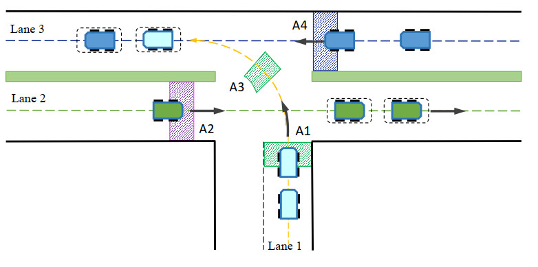
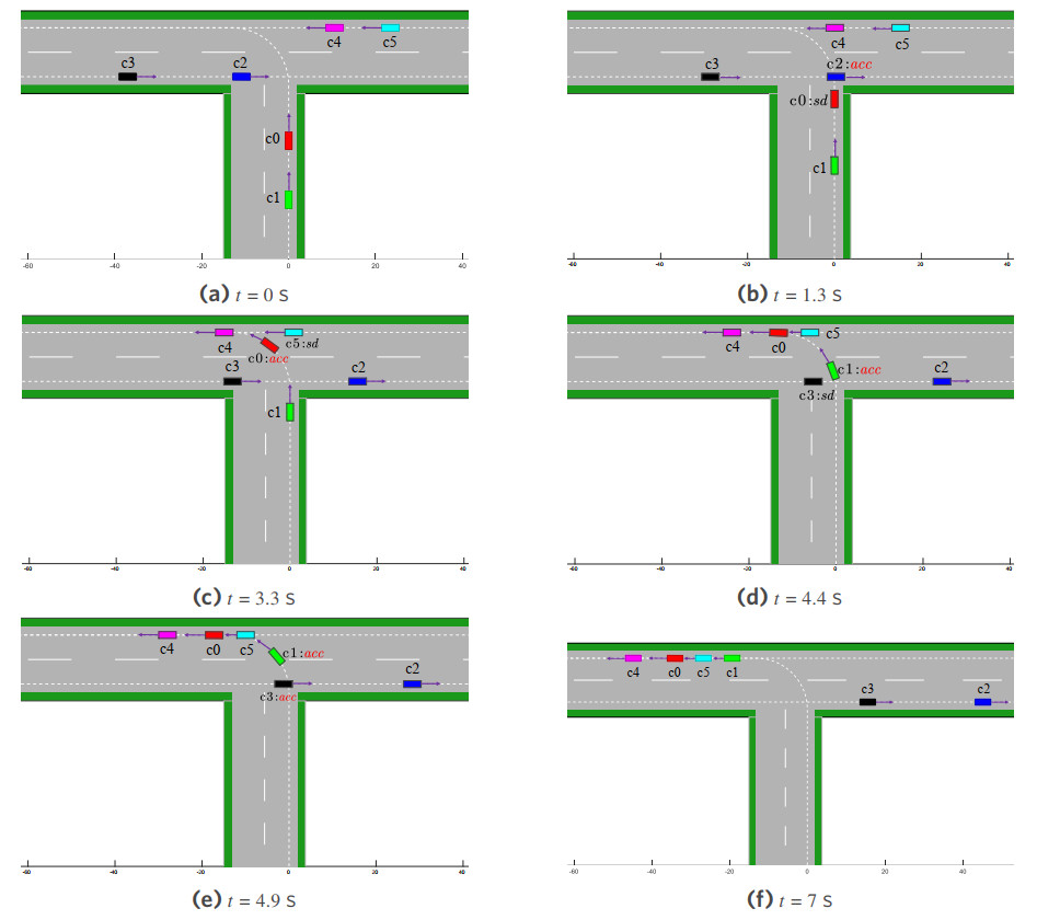
In scenario 1, AVs in Lane 1 perform left turns, while AVs in Lanes 2 and 3 continue straight, as depicted in Figure 5. During navigation, vehicles estimate the motion states of neighboring AVs. By establishing coordination edges with neighbors, they compute optimal actions for safe intersection traversal. The state definitions for AVs in scenario 1 are specified as follows: When an AV in Lane 1 enters decision zone
Figure 5. Illustration of MAVs intersection traversal scenario 1. MAVs: Multiple autonomous vehicles.
During the sampling phase for scenario 1, vehicle states are sampled according to the parameters in Table 1. Each vehicle randomly selects an action (acceleration, deceleration, or maintaining speed) and executes it for 5 s. The updated state vector
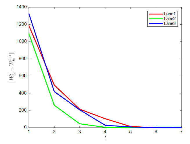
The parameters for local policy learning
| Lane | Kernel width | Iteration error threshold | ||
| Lane 1 | 0.95 | 20 | 0.6 | |
| Lane 2 | 0.95 | 30 | 0.5 | |
| Lane 3 | 0.95 | 5 | 0.5 |
Figure 6. Convergence process of local policy learning via KLSPI. KLSPI: Kernel-based least-squares policy iteration.
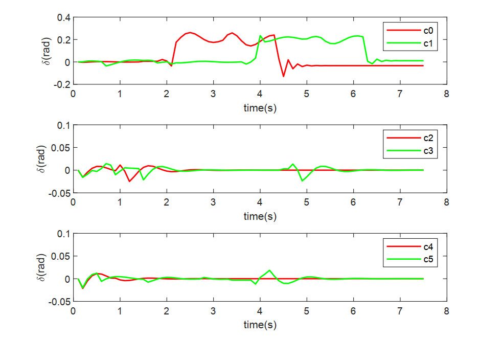
Figure 7. The steering angles of the leading and following AVs on different lanes in scenario 1. AVs: Autonomous vehicles.
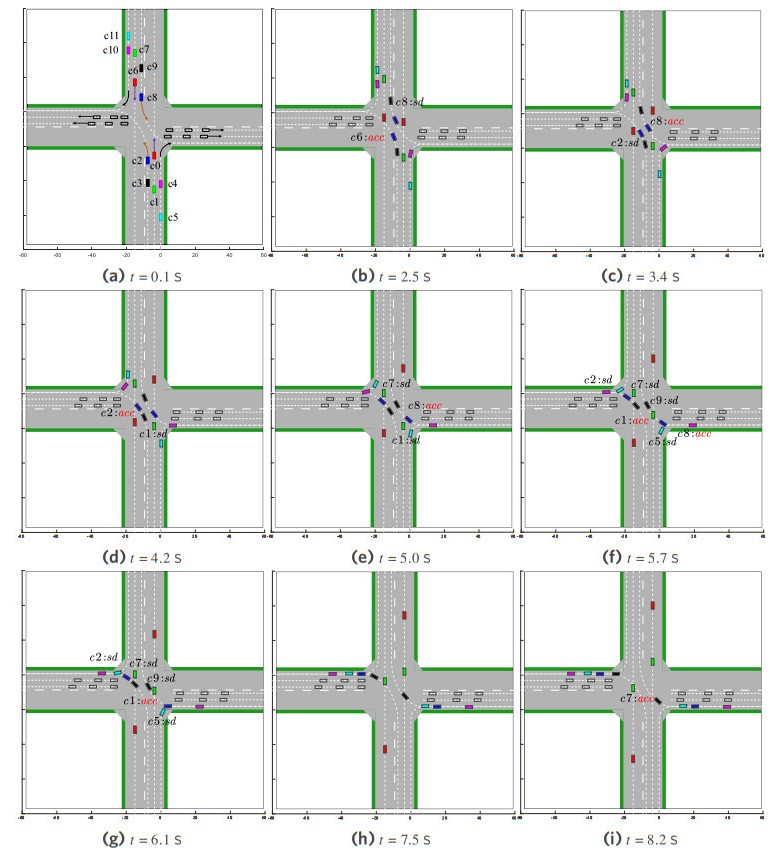
Figure 8 demonstrates the cooperative decision-making and motion trajectories at typical time instants in scenario 1, where sd and acc represent deceleration and acceleration, respectively. Initially, vehicles in each lane are randomly positioned within
Figure 8. The cooperative decision-making and motion trajectories of MAVs at typical time instants in scenario 1. MAVs: Multiple autonomous vehicles.
From Figures 7 and 8, it can be observed that the following vehicles dynamically adjust their acceleration based on the velocity and distance of the leading vehicles, while considering their own speed. This behavior is consistent with the car-following model[35] and effectively prevents collisions.
The performance metrics of the algorithms are statistically analyzed to demonstrate the superiority of the proposed approach. Each algorithm is evaluated over 1, 000 test trials. The performance metrics, including average execution time and its standard deviation, collision rate, failure rate, and comfort level, are presented in Table 3. Traversal time denotes the duration for all vehicles to completely pass the intersection and reach their target lanes. Collision rate counts the percentage of collision occurrences across 1, 000 trials. Failure rate represents the percentage of trials in which vehicles remain within the intersection after 10 s, failing to complete traversal. Comfort is quantified as the average root mean square (RMS) of vehicle accelerations, where lower values indicate higher comfort. Independent learning is a decentralized RL approach in which multiple agents independently learn their state-action value functions without coordination or communication[38], treating others as part of the environment and updating their functions based on individual observations and rewards. The independent learning method[38] deploys identical policies to those in the proposed LCDMC approach, it does not consider the performance of joint actions.
Performance metrics statistics for scenario 1
| Method | Travel time | Collision rate (%) | Failure rate (%) | Comfort | |
| Avg. Time (s) | Std. Dev. | ||||
| LCDMC: Learning-based cooperative decision-making and control. | |||||
| LCDMC | 7.3976 | 0.3340 | 0 | 0 | 0.4877 |
| Independent learning | 8.8453 | 0.8298 | 22.8 | 0.91 | 0.5435 |
As demonstrated in Table 3, the proposed LCDMC method achieves higher traffic throughput efficiency compared to independent learning approaches at unsignalized intersections. This improvement is attributed to LCDMC's cooperative decision-making mechanism, which evaluates joint-action performance through the Max-plus message propagation mechanism, facilitating timely and rational decisions that reduce traversal time. In contrast, in independent learning approaches, vehicles prioritize self-interest by maximizing individual
4.2. Scenario 2: MAVs coordination at a complex unsignalized T-shaped intersection
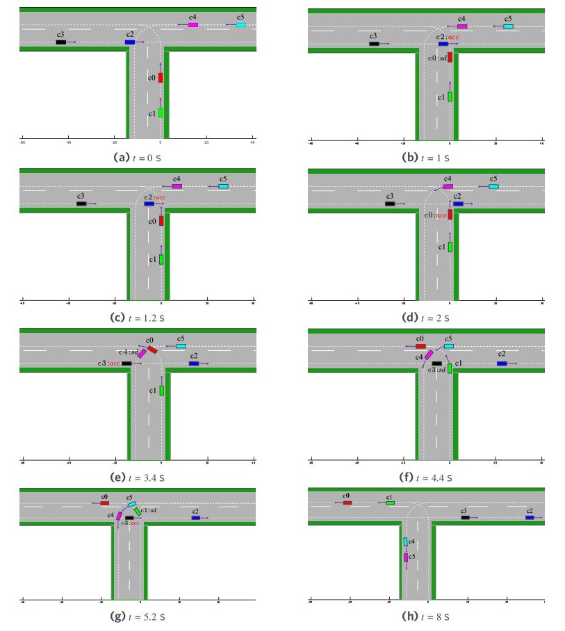
Scenario 2 extends scenario 1 by introducing more complexity in the intersection traffic conditions. In this scenario, AVs in Lane 2 proceed straight, while AVs in Lane 1 and Lane 3 perform left turns, as illustrated in Figure 9. During traversal, AVs in different lanes must consider the motion states of neighboring vehicles to establish cooperative relationships and make rational decisions for safe intersection crossing. The learned policy is deployed in the unsignalized T-junction scenario to evaluate the performance of the LCDMC algorithm. Figure 10 shows the coordinated decision-making and motion trajectories at typical timestamps in scenario 2.
Figure 9. Illustration of MAVs intersection traversal scenario 2. MAVs: Multiple autonomous vehicles.
Figure 10. The cooperative decision-making and motion trajectories of MAVs at typical time instants in scenario 2. MAVs: Multiple autonomous vehicles.
Similar to scenario 1, we conducted 1, 000 test trials for cooperative decision-making for MAVs in scenario 2 to validate the algorithm's superiority. Statistical results of performance metrics are listed in Table 4. The results demonstrate that LCDMC achieves higher traffic throughput efficiency than independent learning at unsignalized intersections. This improvement stems from LCDMC's coordinated decision-making mechanism, which evaluates joint-action performance during policy deployment and leverages message propagation to achieve time-optimal decisions, which reduce traversal time. In contrast, the vehicle action policy in independent learning prioritizes individual rewards, leading to aggressive maneuvers and frequent collisions. LCDMC mitigates this issue through a joint-action utility function that reflects the joint-action performance. Across 1, 000 trials, LCDMC achieved a lower collision rate compared to independent learning. It should be noted that LCDMC's collision avoidance strategy occasionally requires deceleration commands, resulting in slightly worse comfort metrics than independent learning. Overall, the results demonstrate LCDMC's superiority in multi-vehicle coordination efficiency and safety for complex intersection navigation.
Performance metrics statistics for scenario 2
| Method | Travel time | Collision rate (%) | Failure rate (%) | Comfort | |
| Avg. Time (s) | Std. Dev. | ||||
| LCDMC: Learning-based cooperative decision-making and control. | |||||
| LCDMC | 8.1132 | 0.4733 | 0 | 0.1 | 0.8572 |
| Independent learning | 8.9317 | 0.4618 | 27.2 | 4.1 | 0.6110 |
4.3. Scenario 3: MAVs coordination at an unsignalized cross intersection
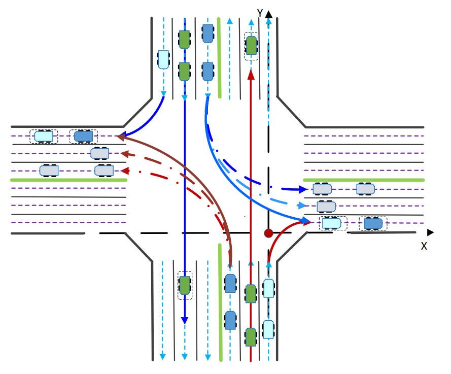
This subsection evaluates the proposed LCDMC algorithm for unsignalized cross intersections. The scenario is illustrated in Figure 11, where AVs perform straight-through, right-turn, and left-turn maneuvers in mixed traffic. Effective navigation requires cross-lane coordination mechanisms to enable optimized decision-making, ensuring safe and efficient crossing. Figure 12 depicts the coordinated decision-making process and resulting motion trajectories at typical time instants in scenario 3.
Figure 11. Illustration of MAVs intersection traversal scenario 3. MAVs: Multiple autonomous vehicles.
Figure 12. The cooperative decision-making and motion trajectories of MAVs at typical time instants in scenario 3. MAVs: Multiple autonomous vehicles.
Subsequently, the performance metrics of different algorithms are calculated to validate the superiority of the proposed approach. Each method undergoes 100 trials, and the performance metrics are recorded in Table 5. The results show that independent learning exhibits a higher standard deviation in traversal time compared to the proposed LCDMC algorithm. Independent learning yields a collision rate of
Performance metrics statistics for scenario 3
| Method | Travel time | Collision rate (%) | Failure rate (%) | Comfort | |
| Avg. Time (s) | Std. Dev. | ||||
| LCDMC: Learning-based cooperative decision-making and control. | |||||
| LCDMC | 11.0440 | 0.3063 | 0 | 0 | 0.7136 |
| Independent learning | 11.8831 | 0.9657 | 26 | 14.5 | 0.7260 |
The LCDMC algorithm integrates KLSPI to compute the local utility function
5. CONCLUSIONS
Aimed at the low traffic efficiency of multi-vehicle navigation at unsignalized intersections, a LCDMC method for MAVs is proposed. LCDMC approach enhances the representational capacity of value functions in multi-agent RL, thereby improving the coordination performance in decision-making and control. The LCDMC algorithm comprises an offline policy learning phase and an online deployment phase. It decomposes the system's global value function into two components: a local state-action value function and a utility function for the joint actions of vehicles. Unlike independent learning methods that solely focus on individual performance, the LCDMC method introduces a coordination graph during the policy deployment phase to effectively characterize the performance of joint actions among MAVs. The optimized policy is derived through iterative message passing among neighboring AVs with cooperative relationships. Moreover, a receding-horizon-based controller is designed, which can enhance the system's real-time performance. Finally, various simulation results demonstrate that the LCDMC method exhibits superior performance in both traffic efficiency and safety for cooperative navigation of MAVs at unsignalized intersections.
DECLARATIONS
Authors' contributions
Made equal contributions to conception and design of the study and simulation and interpretation: Zhang, R.; Xu, X.
Technical and material support, draft improvement: Lu, Y.
Conceptualization, supervision: Xu, X.; Zhang, X.
Supervision, draft improvement: Ma, Q.
Availability of data and materials
The data that support the findings of this study are available from the corresponding author upon reasonable request.
Financial support and sponsorship
None.
Conflicts of interest
Xu, X. (Xin Xu) is Associate Editor of the journal Intelligence & Robotics. Xu, X. (Xin Xu) was not involved in any steps of editorial processing, notably including reviewers' selection, manuscript handling and decision making. The other authors declare that there are no conflicts of interest.
Ethical approval and consent to participate
Not applicable.
Consent for publication
Not applicable.
Copyright
© The Author(s) 2025.
REFERENCES
1. Zhao, J.; Zhao, W.; Deng, B.; et al. Autonomous driving system: a comprehensive survey. Expert. Syst. Appl. 2024, 242, 122836.
2. Tampuu, A.; Matiisen, T.; Semikin, M.; Fishman, D.; Muhammad, N. A survey of end-to-end driving: architectures and training methods. IEEE. Trans. Neural. Netw. Learn. Syst. 2022, 33, 1364-84.
3. Zhang, R.; Sun, C.; Valiollahimehrizi, R.; Czarnecki, K.; Khajepour, A. An uncertainty-aware, dual-tiered decision-making method for safe autonomous driving. IEEE. Trans. Intell. Transport. Syst. 2025, 26, 691-702.
4. Zhao, J.; Knoop, V. L.; Wang, M. Microscopic traffic modeling inside intersections: interactions between drivers. Transp. Sci. 2022, 57, 135-55.
5. Spatharis, C.; Blekas, K. Multiagent reinforcement learning for autonomous driving in traffic zones with unsignalized intersections. J. Intell. Transp. Syst. 2024, 28, 103-19.
6. Reda, M.; Onsy, A.; Haikal, A. Y.; Ghanbari, A. Path planning algorithms in the autonomous driving system: a comprehensive review. Robot. Auton. Syst. 2024, 174, 104630.
7. Li, S.; Peng, K.; Hui, F.; Li, Z.; Wei, C.; Wang, W. A decision-making approach for complex unsignalized intersections by deep reinforcement learning. IEEE. Trans. Veh. Technol. 2024, 73, 16134-47.
8. Al-Sharman, M.; Dempster, R.; Daoud, M. A.; Nasr, M.; Rayside, D.; Melek, W. Self-learned autonomous driving at unsignalized intersections: a hierarchical reinforced learning approach for feasible decision-making. IEEE. Trans. Intell. Transp. Syst. 2023, 24, 12345-56.
9. Xu, Y.; Bao, R.; Zhang, L.; Wang, J.; Wang, S. Embodied intelligence in RO/RO logistic terminal: autonomous intelligent transportation robot architecture. Sci. China. Inform. Sci. 2025, 68, 150210.
10. Li, X.; Liu, K.; Tseng, H. E.; Girard, A.; Kolmanovsky, I. Decision-making for autonomous vehicles with interaction-aware behavioral prediction and social-attention neural network. IEEE. Trans. Control. Syst. Technol. 2025, 33, 1285-300.
11. Guan, Y.; Ren, Y.; Sun, Q.; et al. Integrated decision and control: toward interpretable and computationally efficient driving intelligence. IEEE. Trans. Cybern. 2023, 53, 859-73.
12. Peng, Z.; Wang, Y.; Zheng, L.; Ma, J. Bilevel multi-armed bandit-based hierarchical reinforcement learning for interaction-aware self-driving at unsignalized intersections. IEEE. Trans. Veh. Technol. 2025, 74, 8824-38.
13. Pan, X.; Chen, B.; Timotheou, S.; Evangelou, S. A. A convex optimal control framework for autonomous vehicle intersection crossing. IEEE. Trans. Intell. Transport. Syst. 2023, 24, 163-77.
14. Yuan, M.; Shan, J.; Mi, K. Deep reinforcement learning based game-theoretic decision-making for autonomous vehicles. IEEE. Robot. Autom. Lett. 2022, 7, 818-25.
15. Li, N.; Yao, Y.; Kolmanovsky, I.; Atkins, E.; Girard, A. R. Game-theoretic modeling of multi-vehicle interactions at uncontrolled intersections. IEEE. Trans. Intell. Transport. Syst. 2022, 23, 1428-42.
16. Rizk, Y.; Awad, M.; Tunstel, E. W. Decision making in multiagent systems: a survey. IEEE. Trans. Cogn. Dev. Syst. 2018, 10, 514-29.
17. Mozaffari, S.; Al-Jarrah, O. Y.; Dianati, M.; Jennings, P.; Mouzakitis, A. Deep learning-based vehicle behavior prediction for autonomous driving applications: a review. IEEE. Trans. Intell. Transp. Syst. 2022, 23, 33-47.
18. Wu, Y.; Chen, H.; Zhu, F. DCL-AIM: decentralized coordination learning of autonomous intersection management for connected and automated vehicles. Transp. Res. Part. C. Emerg. Technol. 2019, 103, 246-60.
19. Qian, X.; Altché, F.; Grégoire, J.; de La Fortelle, A. Autonomous intersection management systems: criteria, implementation and evaluation. IET. Intell. Transp. Syst. 2017, 11, 182-89.
20. Liu, J.; Hang, P.; Na, X.; Huang, C.; Sun, J. Cooperative decision-making for CAVs at unsignalized intersections: a MARL approach with attention and hierarchical game priors. IEEE. Trans. Intell. Transp. Syst. 2025, 26, 443-56.
21. Noh, S. Decision-making framework for autonomous driving at road intersections: safeguarding against collision, overly conservative behavior, and violation vehicles. IEEE. Trans. Ind. Electron. 2019, 66, 3275-86.
22. Ebert, J. T.; Gauci, M.; Mallmann-Trenn, F.; Nagpal, R. Bayes bots: collective Bayesian decision-making in decentralized robot swarms. In 2020 IEEE International Conference on Robotics and Automation (ICRA), Paris, France, May 31–Aug 31, 2020. IEEE, 2020. pp 7186–92.
23. EL Bourakadi, D.; Yahyaouy, A.; Boumhidi, J. Multi-agent system based sequential energy management strategy for micro-grid using optimal weighted regularized extreme learning machine and decision tree. Intell. Decis. Technol. 2019, 13, 479–94. https://www.researchgate.net/publication/339188003_Multi-agent_system_based_sequential_energy_management_strategy_for_Micro-Grid_using_optimal_weighted_regularized_extreme_learning_machine_and_decision_tree. (accessed 21 Aug 2025).
24. Gronauer, S.; Dieopold, K. Multi-agent deep reinforcement learning: a survey. Artif. Intell. Rev. 2022, 55, 895-943.
25. Tang, C.; Abbatematteo, B.; Hu, J.; Chandra, R.; Martín-Martín, R.; Stone, P. Deep reinforcement learning for robotics: a survey of real-world successes. Annu. Rev. Control. Robot. Auton. Syst. 2025, 8, 153-88.
26. Wang, S.; Wang, Z.; Jiang, R.; Zhu, F.; Yan, R.; Shang, Y. A multi-agent reinforcement learning-based longitudinal and lateral control of CAVs to improve traffic efficiency in a mandatory lane change scenario. Transp. Res. Part. C. Emerg. Technol. 2024, 158, 104445.
27. Zhang, J.; Chang, C.; Zeng, X.; Li, L. Multi-agent DRL-based lane change with right-of-way collaboration awareness. IEEE. Trans. Intell. Transp. Syst. 2023, 24, 854-69.
28. Wang, T.; Ma, M.; Liang, S.; Yang, J.; Wang, Y. Robust lane change decision for autonomous vehicles in mixed traffic: a safety-aware multi-agent adversarial reinforcement learning approach. Transp. Res. Part. C. Emerg. Technol. 2025, 172, 105005.
29. Hu, X.; Liu, Y.; Tang, B.; Yan, J.; Chen, L. Learning dynamic graph for overtaking strategy in autonomous driving. IEEE. Trans. Intell. Transp. Syst. 2023, 24, 11921-33.
30. Chen, S.; Wang, M.; Song, W.; Yang, Y.; Fu, M. Multi-agent reinforcement learning-based decision making for twin-vehicles cooperative driving in stochastic dynamic highway environments. IEEE. Trans. Veh. Technol. 2023, 72, 12615-27.
31. Chen, D.; Hajidavalloo, M. R.; Li, Z.; et al. Deep multi-agent reinforcement learning for highway on-ramp merging in mixed traffic. IEEE. Trans. Intell. Transp. Syst. 2023, 24, 11623-11638.
32. Guo, Z.; Wu, Y.; Wang, L.; Zhang, J. Heuristic-based multi-agent deep reinforcement learning approach for coordinating connected and automated vehicles at non-signalized intersection. IEEE. Trans. Intell. Transp. Syst. 2024, 25, 16235-48.
33. Zhao, R.; Wang, K.; Li, Y.; Fan, Y.; Gao, F.; Gao, Z. Centralized cooperative control for autonomous vehicles at unsignalized all-directional intersections: a multi-agent projection-based constrained policy optimization approach. Expert. Syst. Appl. 2025, 267, 126153.
34. Li, G.; Yan, J.; Qiu, Y.; et al. Lightweight strategies for decision-making of autonomous vehicles in lane change scenarios based on deep reinforcement learning. IEEE. Trans. Intell. Transport. Syst. 2025, 26, 7245-61.
36. Kok, J. R.; Vlassis, N. Collaborative multiagent reinforcement learning by payoff propagation. J. Mach. Learn. Res. 2006, 7, 1789–828. https://jmlr.org/papers/v7/kok06a.html. (accessed 21 Aug 2025).
37. Guestrin, C.; Lagoudakis, M.; Parr, R. Coordinated reinforcement learning. In Proceedings of the Nineteenth International Conference on Machine Learning, San Francisco, USA. 2002. pp. 227–34. https://cdn.aaai.org/Symposia/Spring/2002/SS-02-02/SS02-02-014.pdf. (accessed 21 Aug 2025).
38. Böhmer, W.; Kurin. V.; Whiteson. S. Deep coordination graphs. arXiv 2019, arXiv: 1910.00091. https://doi.org/10.48550/arXiv.1910.00091. (accessed 21 Aug 2025).
39. Liu, J.; Huang, Z.; Xu, X.; Zhang, X.; Sun, S.; Li, D. Multi-kernel online reinforcement learning for path tracking control of intelligent vehicles. IEEE. Trans. Syst. Man. Cybern. Syst. 2021, 51, 6962-75.
40. Troullinos, D.; Chalkiadakis, G.; Papamichail, I.; Papageorgiou, M. Collaborative multiagent decision making for lane-free autonomous driving. In AAMAS '21: Proceedings of the 20th International Conference on Autonomous Agents and MultiAgent Systems, Richland, USA. 2021. pp. 1335–43. https://dl.acm.org/doi/10.5555/3463952.3464106. (accessed 21 Aug 2025).
Cite This Article
How to Cite
Download Citation
Export Citation File:
Type of Import
Tips on Downloading Citation
Citation Manager File Format
Type of Import
Direct Import: When the Direct Import option is selected (the default state), a dialogue box will give you the option to Save or Open the downloaded citation data. Choosing Open will either launch your citation manager or give you a choice of applications with which to use the metadata. The Save option saves the file locally for later use.
Indirect Import: When the Indirect Import option is selected, the metadata is displayed and may be copied and pasted as needed.
About This Article
Copyright
Data & Comments
Data







Comments
Comments must be written in English. Spam, offensive content, impersonation, and private information will not be permitted. If any comment is reported and identified as inappropriate content by OAE staff, the comment will be removed without notice. If you have any queries or need any help, please contact us at [email protected].