



Morphological analysis and multimodal deep learning for impedance cardiography feature localization and hemodynamic parameter estimation
 0
0 
Abstract
Aim: This study aimed to reduce the susceptibility of impedance cardiography (ICG) feature-point localization to waveform variability, noise, and inter-individual differences by developing an Electrocardiography (ECG)-ICG-phonocardiography (PCG) multimodal framework for beat-to-beat estimation of left ventricular ejection time (LVET), stroke volume (SV), and cardiac output (CO).
Methods: Using the public HeartCycle multimodal dataset, ICG waveform polymorphism and class overlap were characterized using dynamic time warping, K-medoids clustering, and morphological classification. We then developed an end-to-end model with modality-specific one-dimensional convolutional encoders, Transformer-based temporal modeling, and event-query localization. ECG provided beat alignment, and the PCG envelope supplied mechanical-event timing information. Performance was compared with conventional rule-based methods, learning-based baselines, and ablation models under a unified evaluation framework, with paired analyses and leave-one-subject-out (LOSO) validation.
Results: Increasing clustering granularity increased morphological overlap and classification difficulty, indicating limitations of local ICG-only rules. On the primary test set, the PCG-integrated model achieved a mean absolute percentage error of 6.51% for SV and 7.35% for CO, lower than those of the conventional rule-based method and the deep-learning model without PCG. Subject-level paired analyses based on the 17-fold LOSO results demonstrated significant reductions in SV and CO estimation errors following PCG integration and further supported the feasibility of subject-independent beat-level estimation. The complete model also yielded lower errors than learning-based baselines and ablation models under current evaluation conditions. These findings reflect the performance of the integrated framework, while its generalizability warrants further validation.
Conclusion: ECG-ICG-PCG fusion provides a feasible strategy for more stable beat-to-beat LVET, SV, and CO estimation under the current evaluation conditions. Larger multicenter datasets, diverse patient populations, and prospective longitudinal studies are needed to establish reliable trend monitoring and within-subject tracking of hemodynamic changes.
Keywords
INTRODUCTION
In clinical settings such as critical care, perioperative management, and longitudinal follow-up of chronic cardiovascular disease, continuous hemodynamic monitoring is essential for assessing volume status, guiding circulatory support, and evaluating therapeutic efficacy. Compared with invasive approaches, including pulmonary artery catheterization, impedance cardiography (ICG) enables noninvasive, continuous, beat-to-beat hemodynamic assessment by tracking dynamic changes in thoracic electrical impedance throughout the cardiac cycle. Consequently, it has shown considerable promise for monitoring key parameters such as stroke volume (SV), cardiac output (CO), and left ventricular ejection time (LVET). Since the seminal work of Kubicek and colleagues, who introduced a method for estimating CO based on thoracic impedance variations, ICG has been extensively explored in both clinical research and engineering applications, and is increasingly regarded as a promising candidate for wearable, continuous cardiac function monitoring[1-6]. However, the physiological origins of the ICG signal are inherently complex. Its waveform reflects not only aortic blood flow dynamics but also the combined influence of large-vessel volume changes, blood acceleration, and variations in the conductive properties of thoracic tissues[7]. As a result, characteristic points in the ICG waveform do not consistently exhibit a stable one-to-one correspondence with specific mechanical cardiac events. This intrinsic variability renders the computation of ICG-derived hemodynamic parameters highly dependent on the accuracy and robustness of feature-point localization.
Existing studies on key feature points in the ICG waveform, particularly the B and X points associated with aortic valve opening (AVO) and closure, have largely relied on threshold-crossing rules, local extremum detection, template matching, or empirically defined constraints for event localization, from which LVET, SV, and CO are subsequently derived[8-12]. Although such approaches retain a degree of interpretability under ideal signal conditions, they are fundamentally predicated on the assumption that local waveform morphology maps reliably onto the underlying physiological events. In real-world settings, however, respiration, motion artifacts, postural changes, inter-individual variability, and measurement noise can all substantially distort the local structure of the ICG waveform, rendering the definitions of the B and X points increasingly ambiguous and thereby introducing temporal drift or even cross-beat misidentification. In recent years, a number of studies have sought to improve the stability of feature-point extraction by enhancing ICG denoising and signal decomposition through methods such as coherence analysis, canonical correlation analysis, ICEEMDAN, variational mode decomposition (VMD), and related refinements[13-17]. While these techniques can improve signal quality to some extent, most still follow a serial processing paradigm of denoising first, point detection second, and parameter estimation last, such that errors may accumulate progressively across intermediate steps. Moreover, in beat-to-beat estimation and cross-subject generalization, dependence on single-modality ICG waveforms and local morphological heuristics remains insufficient to resolve feature-point ambiguity at its source[18]. Therefore, in ICG analysis, it is not enough to assess whether detected points conform to morphological definitions alone; a more clinically meaningful perspective is to determine whether localization errors propagate downstream and ultimately compromise hemodynamic parameter estimation.
From a physiological perspective, a single-modality ICG signal provides only a limited representation of mechanical ejection events, whereas multimodal physiological signal integration offers a more comprehensive solution. Electrocardiography (ECG) provides a stable reference for the onset of cardiac electrical activity and can serve as a reliable anchor for beat segmentation and inter-cycle alignment. In contrast, phonocardiography (PCG) directly captures mechanical vibrations generated by valve closure and blood flow, with the first and second heart sounds exhibiting well-defined temporal relationships with key systolic mechanical events. As such, PCG has the potential to impose additional constraints on events associated with AVO and closure[19-25]. Compared with single-modality ICG analysis, joint modeling of ECG, ICG, and PCG enables the establishment of a more complete temporal correspondence across electrical activation, mechanical vibration, and impedance variation. This integrated representation can mitigate the uncertainties introduced by noise, morphological distortion, and inter-individual variability, thereby improving the robustness of feature interpretation and downstream hemodynamic assessment.
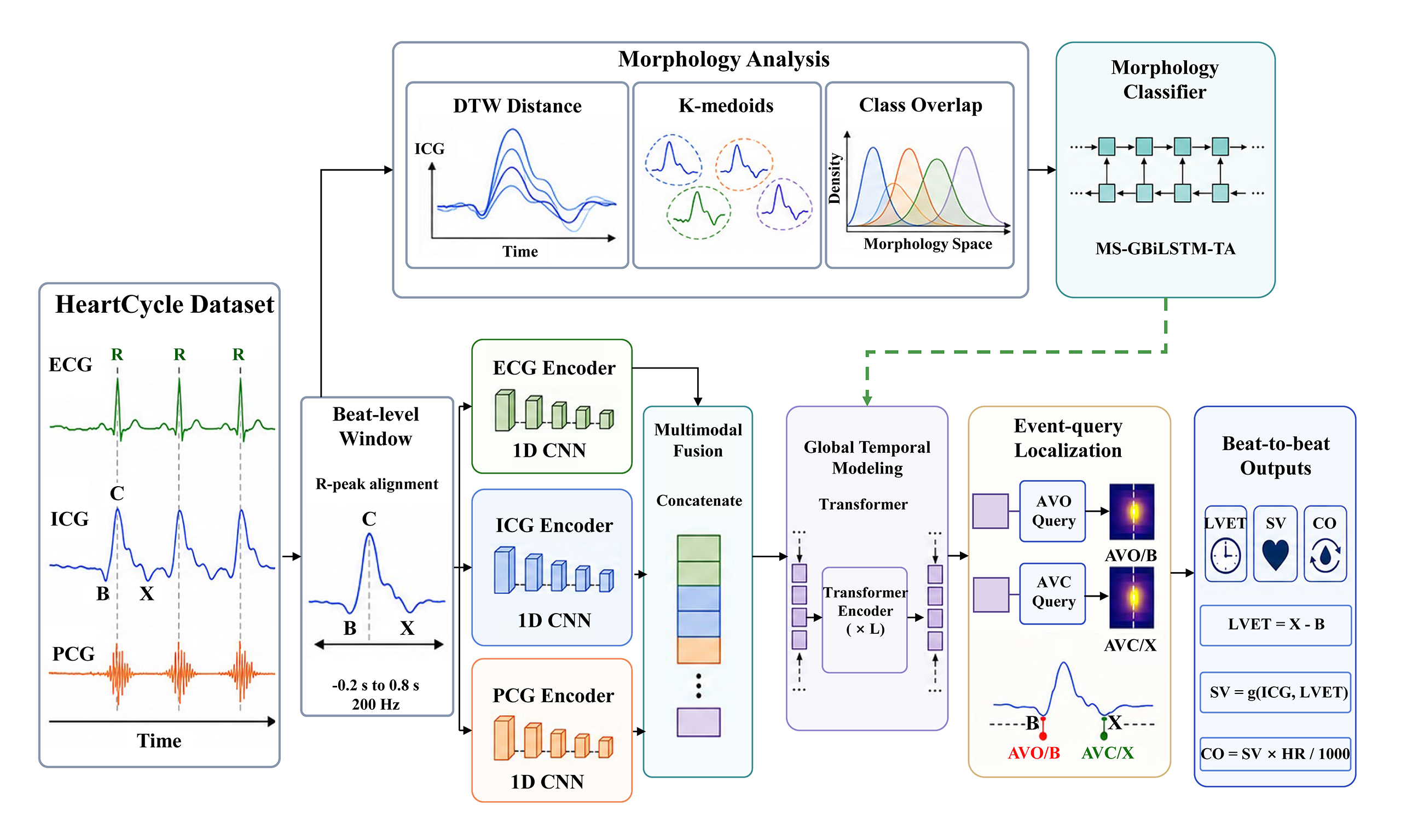
Building on the above considerations, this study establishes an integrated research framework that encompasses ICG waveform morphology analysis and multimodal deep fusion modeling. First, using the HeartCycle multimodal dataset, we conducted a quantitative investigation of ICG waveforms through unsupervised clustering and morphological classification, thereby revealing pronounced morphological heterogeneity and substantial overlap between waveform categories. These findings provide data-driven evidence for the intrinsic limitations of single-modality morphological rules. Second, we developed an end-to-end deep learning model that integrates ECG, ICG, and PCG. In this framework, the PCG envelope is used to provide temporal priors for mechanical cardiac events, while one-dimensional convolutional encoding, Transformer-based global temporal modeling, and an event-query mechanism are jointly leveraged to achieve robust localization of the onset and termination of cardiac ejection. Finally, by introducing an auxiliary regression branch to impose physiological consistency constraints, the localized feature points are further mapped to beat-to-beat estimates of LVET, SV, and CO, enabling a unified comparison between conventional rule-based approaches and multimodal deep learning methods across the entire analytical pipeline. Overall, this work seeks to advance ICG analysis from local morphology-based feature detection toward multimodal modeling optimized for functional parameter estimation, and to provide a methodological foundation for the development of continuous, noninvasive cardiac function monitoring.
MATERIALS AND METHODS
This study established a complete analytical pipeline for ICG feature-point localization and hemodynamic parameter estimation, comprising data preprocessing, waveform morphology analysis, feature-point detection, and parameter derivation. First, using the HeartCycle multimodal dataset, ECG, ICG, and PCG signals were synchronously preprocessed, segmented on a beat-by-beat basis, and normalized to construct a unified beat-level multimodal input. Next, unsupervised clustering and morphological classification were performed on the ICG waveforms to quantitatively characterize their morphological heterogeneity and category overlap. On this basis, the performance of conventional rule-based approaches and deep learning methods was further compared in both key feature-point localization and beat-to-beat hemodynamic parameter estimation. To highlight the contribution of multimodal information - particularly the temporal priors for mechanical events provided by PCG - the study design incorporated multiple comparative settings, including single-modality versus multimodality and rule-based versus learning-based approaches.
Data source and signal preprocessing
This study was conducted using the HeartCycle v1.0.0 multimodal dataset, which is publicly available through PhysioNet (https://physionet.org/content/heartcycle/1.0.0/)[26]. The dataset comprises synchronously acquired signals from 17 healthy subjects, including ECG, ICG, PCG, and ultrasound-derived reference information, as illustrated in Figure 1. These data provide a reliable basis for cardiac cycle-level event localization and hemodynamic parameter evaluation. Unlike studies relying solely on ICG, the HeartCycle dataset offers concurrent observations of electrical activity, mechanical vibration, and impedance variation, making it particularly well suited for multimodal temporal alignment and fusion modeling. All model training, validation, and testing in this study were performed exclusively on this dataset, without the inclusion of external data sources.
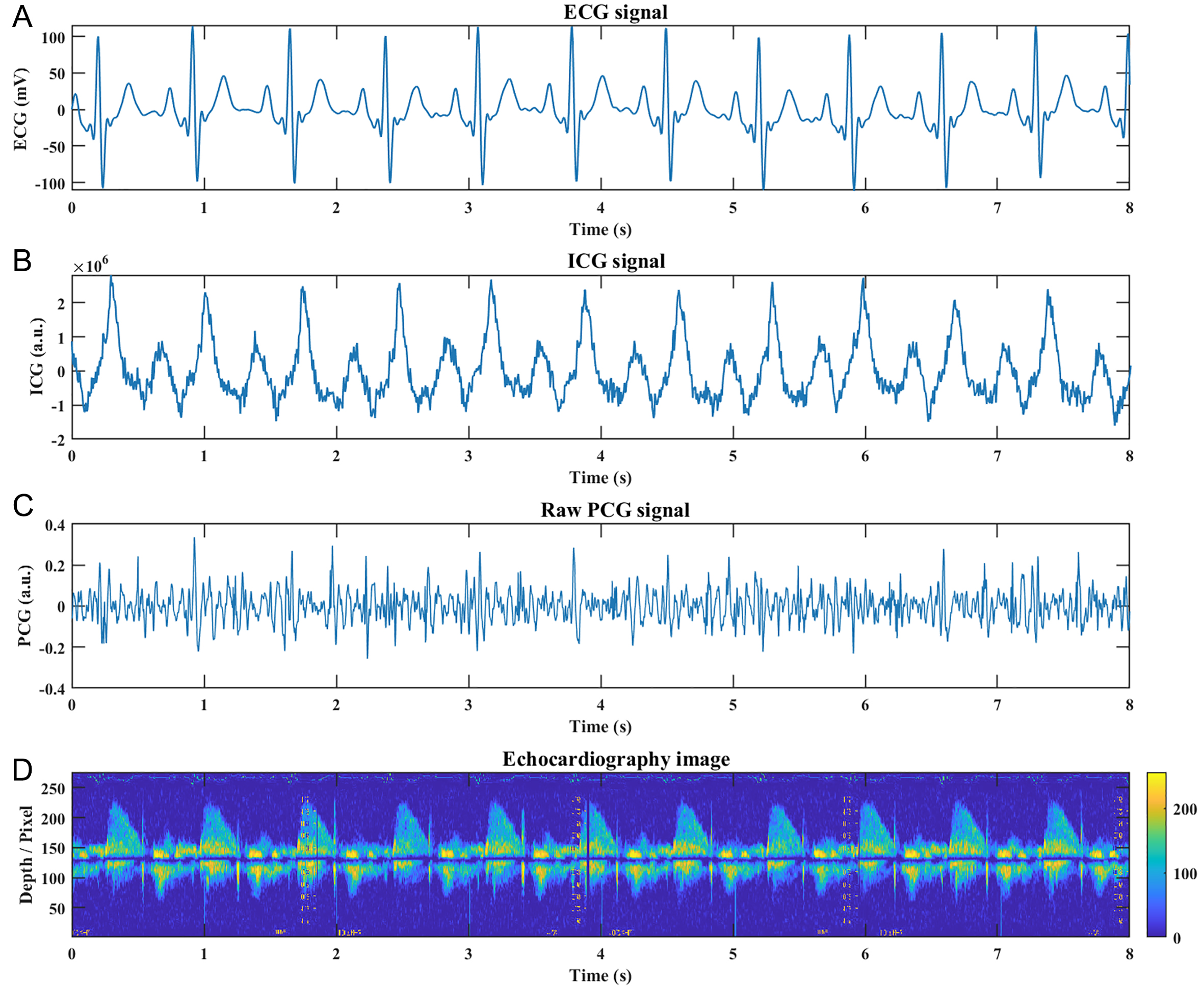
Figure 1. Example of synchronized raw multimodal segments in the HeartCycle dataset: (A) ECG; (B) ICG; (C) PCG; (D) echocardiography.
To preserve physiologically relevant components while suppressing noise, modality-specific preprocessing was performed. For ECG, the conventional rule-based analysis first used a 50 Hz notch filter to suppress power-line interference (Q = 30), followed by a fourth-order Butterworth 0.5-40 Hz band-pass filter to remove baseline wander and high-frequency electromyographic noise. In the deep learning model, ECG was resampled and standardized beat by beat as the temporal reference for electrical activation. For ICG, the conventional morphological analysis first applied a fourth-order Butterworth 0.7-20 Hz band-pass filter to the impedance signal Z, and then used a Savitzky-Golay filter to compute the first derivative dZ/dt[27]. The S-G differentiation window length was 11 samples (approximately 55 ms at 200 Hz), the polynomial order was 3, and the derivative step was delta = 1/200 s. A fourth-order Butterworth 25 Hz low-pass filter was subsequently applied to ICG to suppress residual high-frequency noise. In the deep learning model, the ICG channel was represented by the first gradient of the resampled impedance signal and standardized by z-score normalization within each beat window. For PCG, the conventional ECG + PCG-assisted pipeline used a fourth-order Butterworth 20-200 Hz band-pass filter and smoothed the downsampled amplitude envelope with a 15 Hz low-pass filter. In the deep learning model, PCG was resampled to 4,000 Hz when necessary, filtered using a fourth-order Butterworth 20-800 Hz band-pass filter, transformed into an analytic-signal amplitude envelope by the Hilbert transform[28,29], and resampled to 200 Hz for strict synchronization with ECG and ICG. After single-modality preprocessing, beat-level alignment and segmentation were performed using the ECG R peak as the temporal anchor. The main deep learning model used a fixed input window from 0.20 s before to 0.80 s after the R peak, with a unified sampling rate of 200 Hz, corresponding to 200 time points per beat, as shown in Figure 2. To further reduce the impact of amplitude differences among subjects on subsequent morphological analysis and model training, all segmented heartbeat segments underwent amplitude normalization or z-score standardization. After these steps, a multimodal beat-level input with strict temporal alignment, controlled noise levels, and clear physiological significance was obtained, laying a unified data foundation for subsequent ICG waveform morphological analysis and event localization based on multimodal constraints.
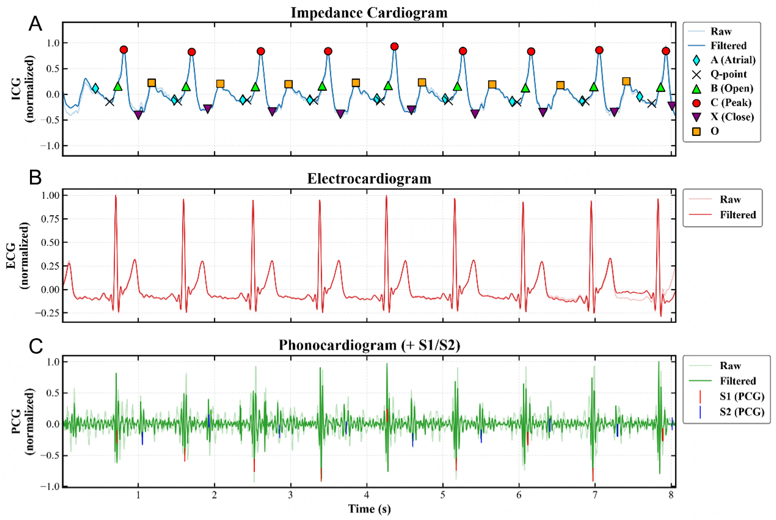
Figure 2. Example of ICG feature-point localization under multimodal denoising constraints: (A) ICG; (B) ECG; (C) PCG.
The reference time points for AVO and aortic valve closure (AVC) were obtained directly from the event annotations publicly released with the HeartCycle dataset rather than manually relabeled in this study. Specifically, the AVO and AVC event coordinates provided in the HeartCycle measurement files were used as the common reference standard for the onset and termination of ventricular ejection. The algorithmic B and X points reported in this study therefore denote feature locations predicted on the ICG waveform by rule-based or learning-based methods, whereas their supervised training and evaluation were based on the dataset-provided AVO and AVC reference labels.
Because the present work relies on public dataset annotations, potential label uncertainty may arise from ultrasound-derived event identification, multimodal synchronization, finite sampling resolution, beat matching, and small timing differences between waveform-derived ICG landmarks and true valvular mechanical events. Such uncertainty can affect feature-point localization and propagate into LVET estimation through the B-X interval. It may also influence downstream SV and CO estimates because these parameters are derived from LVET, heart rate, and ICG morphological descriptors. For this reason, the present study emphasizes parameter-level evaluation in addition to point-localization performance, and reports error distributions, confidence intervals, and paired statistical tests to characterize the impact of label and localization uncertainty on final hemodynamic estimates.
Unsupervised clustering and morphological classification of ICG waveforms
To systematically characterize morphological variation in ICG waveforms across cardiac cycles, unsupervised clustering and morphological classification analyses were performed on the valid preprocessed ICG beat segments. Given that physiological signals commonly exhibit local temporal stretching, phase shifts, and timing misalignment, dynamic time warping (DTW) distance was adopted to quantify waveform similarity and to construct the pairwise distance matrix. Compared with conventional point-to-point Euclidean distance, DTW is better suited for evaluating the overall similarity of ICG waveforms in the presence of temporal fluctuation[30].
Based on the resulting distance matrix, K-medoids clustering was applied to the ICG segments to identify latent waveform morphological subtypes[31]. To examine the distribution of waveform patterns under different levels of clustering granularity, the number of clusters, K, was set to 2, 3, 4, and 5, and the class composition and waveform differences under each clustering scheme were compared. It should be emphasized that the purpose of this analysis was not to establish a fixed clinical taxonomy, but rather to determine, from a data-driven perspective, whether single-modality ICG waveforms exhibit substantial morphological heterogeneity and feature overlap. This analysis also provides a basis for understanding the limitations of conventional rule-based methods in subsequent investigations.
To support both the discovery of ICG waveform morphologies and the evaluation of classification performance, this study conducts unsupervised morphological clustering and supervised classification at two separate levels. First, DTW-K-Medoids clustering is applied to all 1,908 valid ICG beat segments from 17 subjects to characterize the overall morphological heterogeneity of the ICG waveforms in the HeartCycle cohort, identify representative waveforms, and examine the class composition under different numbers of clusters. This step describes the morphological patterns present in the study cohort and defines candidate morphology classes for the subsequent classification tasks. On this basis, the supervised classification experiments adopt a fixed subject-level split to evaluate model generalization to unseen subjects. No subject overlap exists among the training, validation, and test sets, ensuring that multiple beat segments from the same subject do not appear in different data subsets. For each K value, the clustering prototypes, data standardization parameters, and class weights are determined exclusively from the training set. The validation and test sets are transformed, assigned labels, and evaluated using only the parameters obtained during training.
The same fixed subject-level data split is used for all classification tasks with K = 2, K = 3, K = 4, and K = 5 to ensure comparability across different numbers of clusters and model architectures. The training set contains 1,145 beat segments from 11 subjects, the validation set contains 381 beat segments from 3 subjects, and the test set contains 382 beat segments from 3 subjects. The three subsets are completely disjoint at the subject level, and all valid beat segments from each subject are assigned to only one subset. The fixed split comprising 11 training subjects, 3 validation subjects, and 3 test subjects is used exclusively for the ICG morphology classification experiments and is not applied to the subsequent LVET, SV, and CO estimation experiments. Morphology classification and hemodynamic parameter estimation use independent data construction and model training pipelines. Therefore, the subject composition and number of beat segments should be interpreted separately for the two tasks. To prevent information leakage from the test set into model training, all input standardization parameters are estimated using only the training set. Specifically, the mean μtrain(t) and standard deviation σtrain(t) are calculated at each time point t from the training data, and the same training-derived statistics are then used to standardize the training, validation, and test sets. For each K value, the K-Medoids clustering prototypes are fitted using only the training beat segments. Morphology labels for the validation and test segments are determined according to their DTW distances to the training-derived prototypes, with each segment assigned to the nearest prototype. Class weights are also calculated exclusively from the class frequencies in the training set. Let nc denote the number of training samples in class c, and Ntrain denote the total number of training samples. The initial weight for class c is defined as Ntrain/nc, after which all class weights are divided by their mean so that the normalized weights have an average value of 1. These weights are used only in the weighted cross-entropy loss during training, while the class frequencies in the validation and test sets are not involved in their calculation. The validation set is used only for model selection and for saving the model parameters associated with the best validation performance. The test set is evaluated only once after model training and parameter selection are complete.
To further justify the selection of the number of clusters, the clustering results obtained with K = 2, 3, 4, and 5 were evaluated in terms of validity and stability. Specifically, for each value of K, K-Medoids clustering was repeated using five different random seeds, and several clustering validity metrics were calculated, including the Silhouette score, Calinski-Harabasz index, Davies-Bouldin index, inter-/intra-cluster distance ratio, and minimum cluster proportion. To assess the sensitivity of the clustering results to random initialization, the adjusted Rand index (ARI) and normalized mutual information (NMI) were further used to evaluate label consistency across different random seeds. For each value of K, the five repeated clustering runs generated a total of 10 pairwise comparisons, which were used to quantify the consistency and stability of the cluster assignments under different random seeds.
Based on the clustering labels, we further developed an ICG morphology classification model, MS-GBiLSTM-TA, to evaluate the learnability of waveform features under different clustering granularities, as illustrated in Figure 3. The model takes a single ICG segment as input and employs a multi-branch convolutional architecture to extract local morphological features at different scales. A bidirectional long short-term memory network is then used to capture contextual dependencies along the temporal dimension. Subsequently, a temporal attention mechanism is introduced to adaptively weight informative time intervals, thereby enhancing discriminative capability for complex waveform patterns. Because the sample distribution was imbalanced across different clustering schemes, a weighted training strategy was adopted to mitigate the influence of class imbalance on classification performance. By comparing classification results across different clustering granularities, the inter-class separability of ICG waveforms and the clarity of their morphological boundaries could be further assessed.
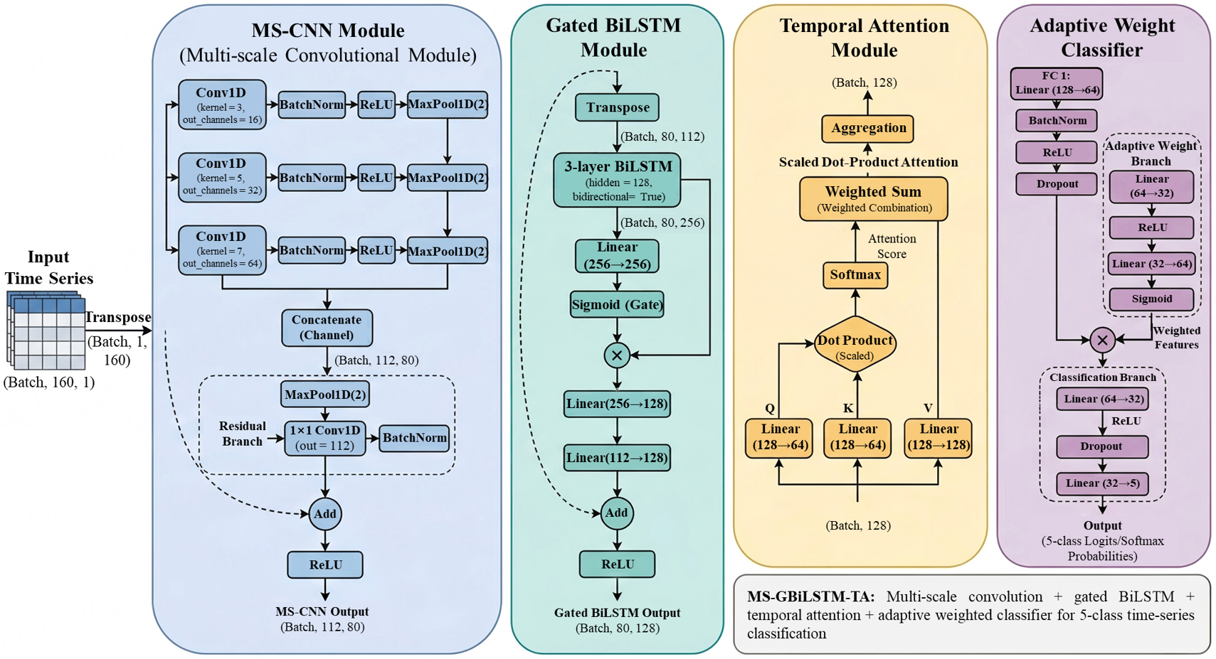
Figure 3. Architecture of the MS-GBiLSTM-TA classification model.
Multimodal feature localization and parameter estimation framework with PCG constraints
This study adopts a single cardiac cycle (beat) as the fundamental unit of analysis. This design is motivated by the intrinsic periodicity of key ICG waveform components, including the systolic upstroke, incisura, and diastolic decay. In both clinical and engineering practice, hemodynamic parameters - such as LVET, SV, and CO - are typically reported on a beat-to-beat basis or through sliding-window averaging. Accordingly, defining model inputs, performing feature-point localization, and deriving parameters at the beat level not only aligns with real-world application requirements but also mitigates the influence of inter-cycle drift on model performance and estimation stability.
For the b-th cardiac cycle, the synchronized multimodal input segment is defined as
where
This study compares four feature-point localization strategies, each formulated in a unified manner as a mapping from multimodal inputs to the temporal positions of key feature points. For the b-th cardiac cycle, the m-th localization strategy can be expressed as
where fm(·) denotes the m-th feature-point localization strategy, and
To avoid conceptual ambiguity, it should be clarified that the B and X points referred to in this study primarily represent the feature-point locations identified on the ICG waveform by the proposed model or rule-based method. Both supervised training and performance evaluation used the publicly available AVO and AVC event timestamps as reference labels in the HeartCycle dataset. Therefore, the algorithm-derived B and X points were not treated as independently annotated ground-truth labels. Instead, the AVO and AVC reference labels were used as unified reference standards for the onset and termination of ventricular ejection, respectively, against which ICG feature-point localization and LVET estimation were evaluated. It should be noted that there may be systematic deviations between the B/X annotation and the actual valve event. For example, changes in waveform morphology may lead to different algorithms having inconsistent definitions of point B. Accordingly, point-wise localization error alone is insufficient to fully capture the practical value of a given method. A more meaningful evaluation is to examine whether such localization errors materially affect the final hemodynamic estimates, which is precisely why this study places greater emphasis on parameter-level performance. After obtaining
Subsequently,
Finally, CO is computed from the corresponding heart rate HR(b) for that beat:
Specifically, the ICG morphological descriptor for each cardiac beat was defined as the absolute peak amplitude of the ICG signal at the systolic C point. Its detailed definition and parameter-calibration procedure are provided in Section “Parameter derivation and evaluation metrics”. To ensure a fair comparison across methods, all experiments employed the same parameter derivation function, g(·), thereby minimizing the influence of subsequent parameter-conversion procedures. Accordingly, performance differences between methods were intended to primarily reflect their ability to localize ICG fiducial points.
Conventional rule-based localization method
The conventional approach follows a rule-based ICG feature-point localization pipeline. Cardiac cycles are segmented at the beat level using the ECG R peak as the temporal anchor. The overall workflow is illustrated in Figure 4.
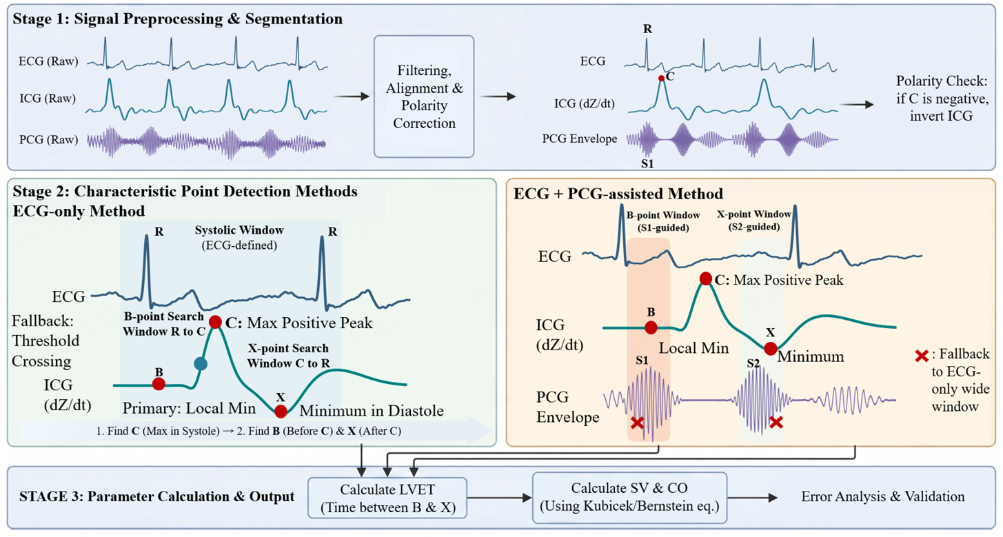
Figure 4. Workflow of the conventional rule-based feature-point localization method.
Within each cardiac cycle, the systolic dominant peak (C point) is first identified on the ICG waveform to establish the principal systolic morphology. Subsequently, the feature points associated with AVO and closure - the B point and X point, respectively - are searched within predefined intervals before and after the C point. The LVET is then obtained as the temporal difference between B and X, and is further used to derive SV and CO. To reduce the temporal ambiguity associated with localization based solely on ICG morphology, we design two conventional localization strategies. The first uses only the rhythm information provided by ECG to constrain the search windows for the B and X points. The second further incorporates the mechanical-event timing priors provided by S1 and S2 in the PCG to narrow the candidate search intervals for the B and X points, without directly treating S1 and S2 as the corresponding B and X points. These strategies reduce uncertainty in fiducial point searching and improve localization stability and robustness under noise interference, interindividual variability, and changes in waveform morphology.
ECG-only method
As a baseline for conventional feature-point localization, this approach relies exclusively on ECG-derived electrical activity as the physiological anchor to constrain the search space for ICG features. Specifically, R peaks are first detected from the ECG using a modified Pan-Tompkins algorithm[10], and the continuous recordings are segmented into individual cardiac cycles based on these fiducial points. Feature-point localization is then performed in a sequential manner within each beat.
The systolic dominant peak (C point), corresponding to the moment of maximal left ventricular ejection velocity, is first identified. The algorithm searches for the global maximum of the ICG waveform within a predefined systolic window following the R peak. Accurate localization of the C point establishes a reliable temporal and amplitude reference for subsequent steps. The B point, physiologically associated with AVO and marking the onset of ejection, is then determined. Given inter-individual variability in the pre-ejection period and the frequent distortion of the ICG upstroke due to baseline drift or superimposed noise, the algorithm first searches for a local minimum on the upstroke within an adaptive window between the R peak and the C point, selecting the trough closest to the leading edge of the C point. However, because morphological variability often renders such minima indistinct or absent, a robust threshold-crossing fallback strategy is introduced. When no stable minimum is detected, a fixed proportion of the C-point amplitude is used as an adaptive threshold, and the first upward crossing of this threshold along the rising limb is taken as a surrogate for the B point.
Finally, the X point, corresponding to AVC and the termination of ejection, is localized. In a typical ICG waveform, this point appears as a pronounced dicrotic notch spanning late systole to early diastole. The algorithm identifies the absolute minimum within the interval between the C point and the subsequent R peak. To prevent misclassification of later diastolic features - such as the O wave (associated with mitral valve opening) - or structures from the next cardiac cycle, a strict physiological constraint is imposed on the upper bound of the search window, thereby effectively reducing cross-cycle localization drift.
ECG + PCG-assisted method
Because localization based solely on single-modality ICG morphology is highly susceptible to temporal ambiguity under complex conditions, the ECG + PCG-assisted method incorporates PCG as prior information related to cardiac valve mechanical events. Heart sounds capture acoustic manifestations of valve closure and hemodynamic impact. The first heart sound, S1, occurs near the isovolumetric contraction phase and is temporally associated with the B point, corresponding to AVO. The second heart sound, S2, is primarily generated by the closure of the aortic and pulmonary valves and therefore provides an important mechanical timing cue for anchoring the X point, corresponding to AVC. To achieve temporal coordination across modalities, the PCG signal is first subjected to tailored preprocessing. After bandpass filtering to suppress respiratory sounds and low-frequency artifacts, the signal amplitude is converted to its absolute value and smoothed using a low-pass filter, or the Hilbert transform is applied to extract the heart sound energy envelope. Within each R-R interval, an adaptive peak detection algorithm is then used to identify the energy centers of S1 and S2. Spurious peaks caused by environmental noise are further removed using energy thresholds and empirically defined temporal windows.
The PCG signal is first processed using a 20-200 Hz fourth-order Butterworth bandpass filter. After taking the absolute amplitude, the signal is downsampled to approximately 1,000 Hz, and a 15 Hz fourth-order low-pass filter is applied to obtain a normalized energy envelope. The amplitude threshold for high-confidence heart sound peaks is defined as the envelope median plus six times the median absolute deviation. The lower bound of the S1 search window is set to 20 ms after the Q point. When the Q point is unavailable, the lower bound is set to 20 ms after the R peak. The upper bound is defined as min(200 ms after the R peak, 300 ms before the next R peak). The S2 search window extends from max(150 ms after S1, 200 ms after the R peak) to min(50 ms before the next R peak, 650 ms after the R peak, 0.75RR after the R peak). S1 or S2 is marked as a reliable event, and the corresponding temporal constraint is activated, only when the candidate peak exceeds the amplitude threshold. Otherwise, the constraint associated with that heart sound event is removed, and the algorithm reverts to the ECG-only search rules. When S1 is reliable, the B-point search window is defined from max(10 ms after the R peak, 10 ms after the Q point, 5 ms after S1) to min(350 ms after the R peak, 20 ms before the C point, 180 ms after S1), with the center of the temporal proximity score set to 60 ms after S1. For B-point candidate minima, the minimum separation is set to 30 ms, the prominence threshold is set to 0.04 times the standard deviation of the candidate interval, and the width of the temporal proximity score is set to 50 ms. If no valid local minimum is identified, the algorithm retains the threshold-crossing rule based on 15% of the C-point amplitude to detect the B point on the ascending limb. When S2 is reliable, the X-point search window is defined from max(50 ms after the C point, 80 ms before S2) to min(50 ms before the next R peak, 0.90RR after the R peak, 900 ms after the R peak, 160 ms after S2), with the center of the temporal proximity score set to 20 ms after S2. For X-point candidate minima, the minimum separation is set to 30 ms, the prominence threshold is set to 0.03 times the standard deviation of the candidate interval, and the width of the temporal proximity score is set to 80 ms. If no local minimum satisfies these criteria, the absolute minimum within the constrained interval is selected. When S1 or S2 is unreliable, localization of the corresponding B or X point automatically reverts to the wide-window ECG-only rules.
Multimodal event localization based on deep learning
This study reformulates the ICG fiducial point localization problem as a deep learning-based sequence modeling task. The proposed framework automatically learns the temporal patterns associated with AVO and closure events from multimodal signals, including ECG, ICG, and PCG, in a data-driven manner, thereby improving the stability of fiducial point localization under complex waveform conditions. The overall workflow is illustrated in Figure 5. The primary advantage of the deep learning approach lies in its ability to extract high-level representations directly from raw signals and to integrate complementary information across modalities within an end-to-end architecture, thereby reducing reliance on handcrafted rules and prior assumptions inherent to conventional methods. In this section, the proposed model is described in detail, including its input representation, network architecture, training strategy, and inference procedure.
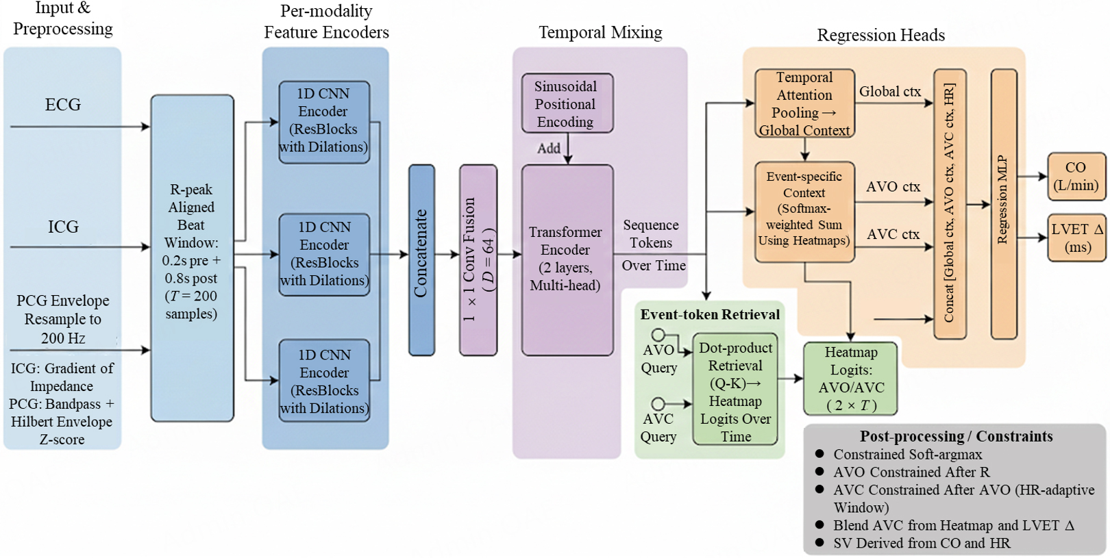
Figure 5. Workflow of the proposed deep learning-based method.
For each cardiac cycle, the ECG R peak was used as the temporal anchor, and multimodal signal segments from 0.20 s before to 0.80 s after the R peak were extracted to construct a fixed 1.00 s beat-level analysis window. This window covers the main physiological process from electrical activation to the end of mechanical systole and includes the typical temporal range of the B and X points. To ensure temporal consistency across modalities and reduce computational complexity, all signals were resampled to 200 Hz; therefore, each beat-level input sample contained 200 time points. The ECG signal was z-score standardized beat by beat after resampling and used as the electrical timing reference. The ICG signal was represented by its first derivative, computed as the temporal gradient of the resampled impedance signal and then z-score standardized within each beat, to emphasize rapid hemodynamic waveform changes. For PCG, when the original sampling rate was high, the signal was first resampled to 4,000 Hz, then filtered using a fourth-order Butterworth 20-800 Hz band-pass filter, transformed into an analytic-signal amplitude envelope using the Hilbert transform, resampled to 200 Hz, and standardized within each beat. Compared with the raw high-frequency PCG waveform, the envelope representation preserves key valvular acoustic events such as S1 and S2 while reducing training instability caused by high-frequency oscillations.
To fairly evaluate the contribution of PCG, two input configurations were evaluated: a trimodal setting (ECG + ICG + PCG) and a bimodal setting (ECG + ICG, with the PCG channel set to zero). The network architecture was kept identical between settings so that performance differences could be attributed to information content rather than model capacity. The proposed deep learning model consists of four core components: modality-specific encoders, a multimodal fusion and contextual modeling module, an event-query localization head, and an auxiliary regression constraint module. The model was designed to capture both local waveform morphology and global temporal dependencies, while introducing physiological consistency constraints into the localization task. To avoid mixing the different statistical properties of the modalities too early, an independent one-dimensional convolutional encoder was assigned to each modality. Each encoder maps a single-channel sequence to a high-dimensional feature representation:
Each encoder consists of an initial stem convolutional layer with kernel size 7, followed by stacked residual dilated convolutional blocks. The residual blocks use convolutions with kernel size 5 and a dilation-rate sequence of [1, 2, 4, 8, 16, 8, 4, 2], forming a multi-scale receptive field that captures millisecond-level local waveform details and broader morphological context over hundreds of milliseconds. The three modality-specific feature representations are then concatenated along the channel dimension and projected into a shared latent space with hidden dimension d = 64 through a convolutional layer, yielding the fused temporal representation:
The fused representation is transposed into a temporal-token sequence and combined with sinusoidal positional encoding to inject absolute timing information. The resulting sequence is passed to a module composed of two Transformer encoder layers, whose self-attention mechanism captures long-range dependencies across the entire cardiac window:
In the event localization head, an event-query retrieval mechanism was adopted to jointly exploit the complementary temporal information provided by ECG, ICG, and PCG signals. Specifically, the model defines two learnable event query vectors,
where s is a learnable scaling parameter and be is the event-specific bias term. This yields a logit heatmap
In addition to the primary localization task, the model incorporates an auxiliary regression branch to impose physiological consistency constraints. First, an additive temporal attention module is applied to H obtain a global context vector,
where σ corresponds to a temporal tolerance of approximately 18 ms (converted into sample points according to the sampling rate), which helps mitigate annotation jitter and provides more stable gradients during training. The heatmap localization loss is implemented using focal binary cross-entropy with logits to address the extreme class imbalance along the temporal axis between positive samples (event locations) and negative samples (non-event time points).
For the regression task, predictions of CO and ΔLVET were optimized using the Smooth L1 (Huber) loss, with missing labels masked during training. To further enforce internal physiological consistency, the model derived the predicted SV from the predicted mean
During inference, the heart rate used to calculate the RR interval is constrained to 30-220 beats/min. The AVO heatmap decoding window extends from 15 ms after the R peak to min(250 ms, 0.55RR) after the R peak. The lower bound of the AVC decoding window is set to 80 ms after AVO, and the upper bound is set to min(750 ms, 0.85RR) after AVO. Heatmap logits outside these intervals are masked, and the event positions from the heatmap branch are calculated within the constrained intervals using soft-argmax with a temperature parameter of τ = 0.35. The LVET predicted by the auxiliary regression branch is constrained to 120-650 ms and is used to construct a second AVC candidate, defined as the AVO position plus the auxiliary LVET. This candidate is further constrained to the same physiological AVC interval used by the heatmap branch. The AVC heatmap confidence is defined as the maximum probability obtained after temperature-based normalization with τ = 0.35 within the constrained AVC interval. The final AVC position is obtained by fusion according to AVCfinal = (1 - w)AVCheatmap + wAVCaux. When the heatmap confidence is below 0.18, the fusion weight w for the auxiliary LVET pathway is set to 0.45. When the confidence is at least 0.18, w is set to 0.20. The corresponding weights of the heatmap branch are therefore 0.55 and 0.80, respectively. These search ranges, thresholds, and fusion weights remain fixed across all training and test folds, and neither the validation set nor the test set is used to determine these values.
The primary hemodynamic parameter estimation experiment uses a fixed subject-disjoint data split. The training set includes CH08 and CH09, with 152 candidate beat segments in total, comprising 52 segments from CH08 and 100 from CH09. The validation set includes CH10 with 59 candidate beat segments, while the test set includes CH07 with 70 candidate beat segments. After filtering for complete reference labels, 61 valid test beats with reference values for LVET, SV, and CO are retained for unified beat-level performance evaluation in the main experiment. No subject overlap exists among the training, validation, and test sets. These 61 beats are used only to report beat-level performance on the fixed test set and are not treated as independent samples in the subsequent paired statistical analysis involving 17 subjects. Subject-level inference is conducted separately using independent test results obtained when each subject is completely held out in the 17-fold leave-one-subject-out (LOSO) evaluation.
To evaluate computational efficiency, the forward inference time and parameter number of the Proposed model are measured on a Windows 10 workstation. The evaluation environment includes an Intel Core i7-14650HX CPU, an NVIDIA GeForce RTX 4060 Laptop GPU, Python 3.11.14, and PyTorch 2.5.1. The Proposed model contains 395,270 parameters, and the checkpoint file size is approximately 1.65 MB. The model input is a beat-level multimodal signal segment with a length of 1 s, consisting of 200 temporal points and three channels. On the CPU, the average forward inference time for a single heartbeat window is 23.72 ± 3.69 ms with a batch size of 1, corresponding to 1.62 ms/beat with a batch size of 64. On the GPU, the average inference time is 6.24 ± 1.13 ms for batch size 1 and 0.15 ms/beat for batch size 64. These results indicate that the proposed model has a low computational burden and can support beat-level offline analysis and near-real-time processing.
To further compare the performance of different learning-based models, three baseline models, including CNN-only, BiLSTM, and ICG-only, are established using the same beat-level data partitioning, input modalities, preprocessing procedures, and evaluation metrics as the main experiment. The CNN-only baseline employs conventional one-dimensional residual convolution for feature extraction and heatmap localization without incorporating the event-token attention mechanism. The BiLSTM baseline uses bidirectional LSTM networks to model temporal dependencies and estimates LVET only from AVO/AVC heatmap localization results without an additional direct LVET regression head. Both learning-based baselines use ECG, ICG (dZ/dt), and PCG envelope as multimodal inputs and follow the same training epochs, validation-based model selection strategy, and test evaluation procedure. In addition, an ICG-only baseline model is introduced to investigate the limitations of single-channel ICG-based localization and parameter estimation. This model maintains the same data partitioning, R-peak alignment windows, preprocessing pipeline, training epochs, validation selection strategy, and test evaluation procedure as the main experiment. However, it only uses single-channel ICG signals as input and does not incorporate ECG waveform information, PCG envelope features, or the event-token attention mechanism. The ICG-only model directly predicts AVO/AVC heatmaps from the single-channel ICG representation, and LVET is calculated from the detected fiducial points. SV and CO are subsequently obtained using the same output conversion procedure as other learning-based models.
Parameter derivation and evaluation metrics
To ensure fair comparison among localization strategies, the same hemodynamic parameter derivation pipeline was used for all methods. Regardless of whether the method was rule-based (ECG-only or ECG + PCG-assisted) or deep learning-based (DL w/o PCG or DL + PCG), each method first produce the B-point and X-point locations for every valid cardiac cycle, and LVET, SV, and CO were then calculated using the same deterministic post-processing procedure. The auxiliary regression branch in the deep learning model was used only to impose physiological consistency during training and to assist decoding for low-confidence samples during inference; it was not used directly as the source of the final reported SV and CO results.
For the i-th valid cardiac cycle, if the B and X points output by the model are first represented as sample indices, they are converted to the physical time axis according to the sampling rate:
On this basis, left ventricular ejection time is defined as:
After obtaining
The absolute peak amplitude of ICG at the C point was then defined as:
Here, AC(b) denotes the only ICG morphological descriptor used in this study for SV derivation. No waveform integral, area-based measure, second-derivative feature, template similarity measure, or other manually engineered ICG morphological indices were used. The
As the HeartCycle dataset does not provide the complete subject-specific parameters required by conventional Kubicek or Sramek-Bernstein equations, including thoracic length, electrode spacing, baseline impedance, and blood resistivity, fixed constants reported in the literature were not directly adopted. Instead, the scaling coefficient KSV was robustly calibrated once within each training split using the VE reference sequence provided by HeartCycle. Specifically, the VE time series was first linearly interpolated at the timing of the current R peaks to obtain beat-wise reference SV values:
The reference ejection time was calculated from the public AVO and AVC reference events:
In the valid training-beat set
To reduce the influence of aberrant cardiac beats, outliers were first removed within the training set based on the median absolute deviation of logr(b), yielding the valid set
Accordingly, the predefined beat-level SV function g(∙) used in this study was:
Heart rate was obtained from adjacent R-R intervals:
Finally, CO was calculated as:
Here,
Let
Based on the above definitions, this study calculates the MAPE values for LVET, SV, and CO and evaluates ECG-only, ECG + PCG-assisted, DL w/o PCG, and DL + PCG using a unified parameter derivation procedure and consistent evaluation metric definitions. Because the number of valid beats available for parameter evaluation after filtering for complete reference labels differs across methods, cross-category comparisons between the conventional rule-based and deep learning methods are presented primarily as descriptive analyses. Method comparisons and statistical inference based on the same set of valid beats are conducted separately in the corresponding controlled experiments. MAPE was selected as the primary metric because the magnitudes of SV and CO can differ substantially among subjects; percentage error reduces the influence of scale differences on the overall statistics and better reflects the relative impact of feature-point localization errors on final functional parameter outputs.
RESULTS
Morphological clustering results and data distribution characteristics of ICG waveforms
To quantify the intrinsic complexity of ICG waveform morphology, unsupervised clustering was first performed on 1,908 valid ICG beat segments extracted from the HeartCycle dataset. The clustering results provide an intuitive representation of the morphological diversity of ICG waveforms as well as the distributional differences across clusters. In the waveform visualizations, solid lines represent the mean morphology of each cluster, while the shaded regions indicate the mean ± one standard deviation (±SD), thereby illustrating intra-class variability and the extent of feature overlap between different clusters. The corresponding visualization results are shown in Figure 6.
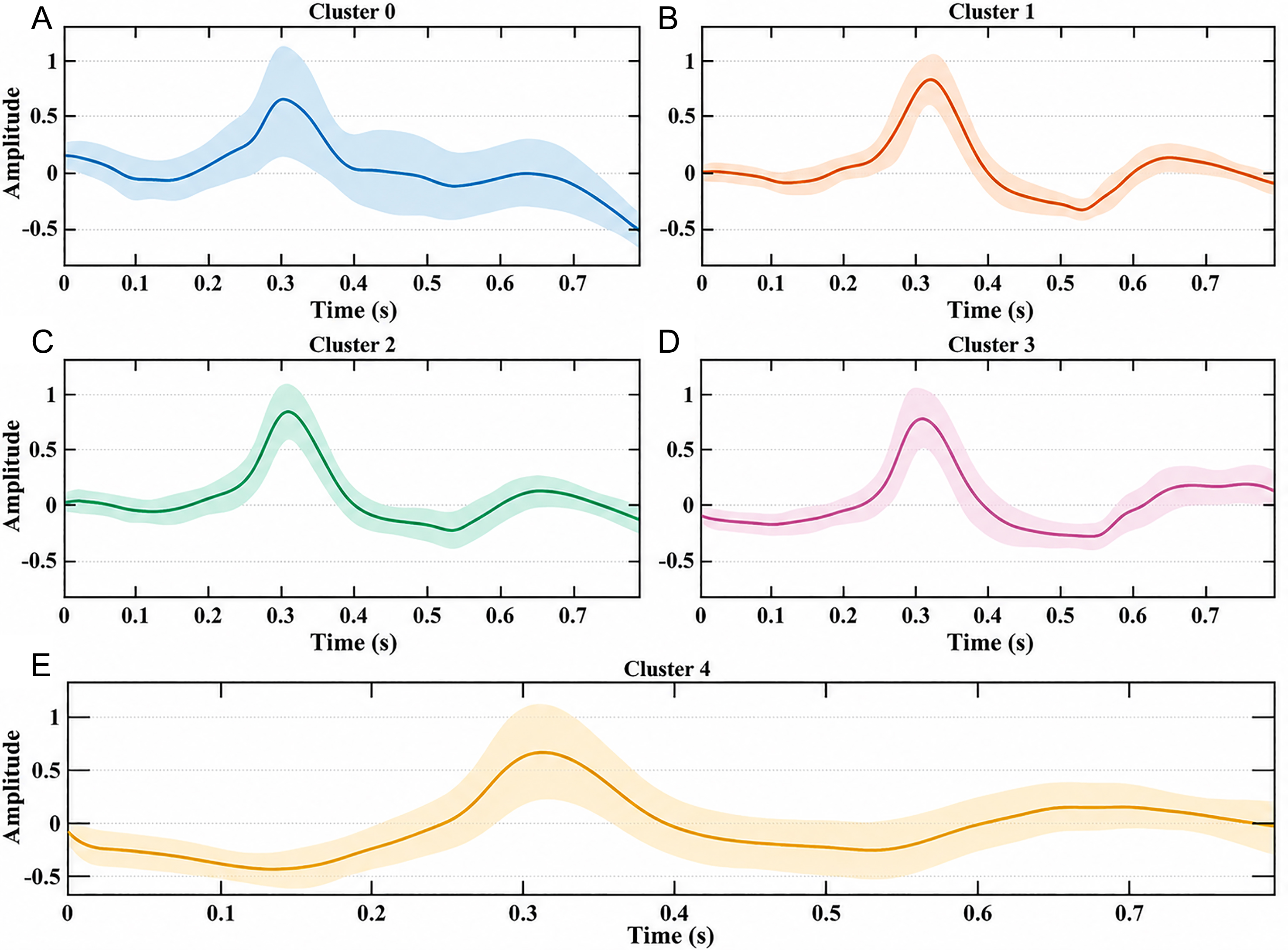
Figure 6. ICG waveform morphology of the HeartCycle dataset under the K = 5 clustering scheme. A total of N = 1,908 valid ICG beat segments are included. (A-E) correspond to Cluster 0-4, with sample sizes of n = 297, 340, 526, 612, and 133, respectively. The solid line represents the mean normalized ICG waveform of each cluster, and the shaded region indicates the mean ± SD.
The statistical results are summarized in Figure 7. A total of 1,908 valid ICG segments from the HeartCycle dataset were included in the clustering analysis. For K = 2, the two clusters contained 625 and 1,283 segments, respectively. For K = 3, the cluster sizes were 818, 484, and 606 segments. For K = 4, the distribution further split into 713, 670, 430, and 95 segments. For K = 5, the cluster sizes were 297, 340, 526, 612, and 133 segments. Across both coarse- and fine-grained clustering settings, pronounced class imbalance was consistently observed. These results indicate substantial morphological heterogeneity of ICG waveforms across cardiac cycles, accompanied by significant inter-class overlap. As clustering granularity increases, both boundary ambiguity between clusters and imbalance in class distribution become more evident. These findings suggest that conventional feature-point localization methods based on single-modality local morphological rules are unlikely to generalize robustly across diverse waveform patterns.
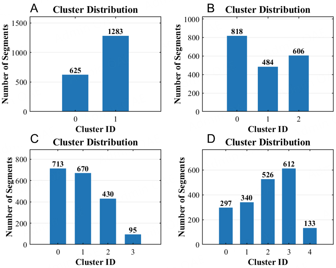
Figure 7. Cluster sample size distribution of the HeartCycle dataset under different numbers of clusters K. A total of N = 1,908 valid ICG beat segments are included. (A-D) correspond to K = 2, K = 3, K = 4, and K = 5, respectively. The bar height and the values displayed above each bar indicate the number of beat segments contained in the corresponding cluster.
To further justify the choice of cluster number, the validity and stability of K = 2-5 clustering solutions were evaluated using internal validity metrics and repeated random seeds. K = 2 achieved the best global geometric separation according to the Silhouette, Calinski-Harabasz, and Davies-Bouldin indices, suggesting a coarse two-pattern structure in the ICG waveforms. However, K = 3 showed the highest cross-seed stability (ARI, 0.777 ± 0.145; NMI, 0.796 ± 0.116) while maintaining an interpretable minimum cluster proportion of 24.916% ± 0.368% without extremely small clusters. In contrast, K = 4 and K = 5 showed smaller minimum-cluster proportions and a higher risk of over-partitioning. Therefore, K = 3 was considered more suitable for subsequent morphology-stratified analysis when geometric separation, stability, and cluster-size interpretability were considered jointly. The quantitative results are summarized in Table 1 and Figure 8.
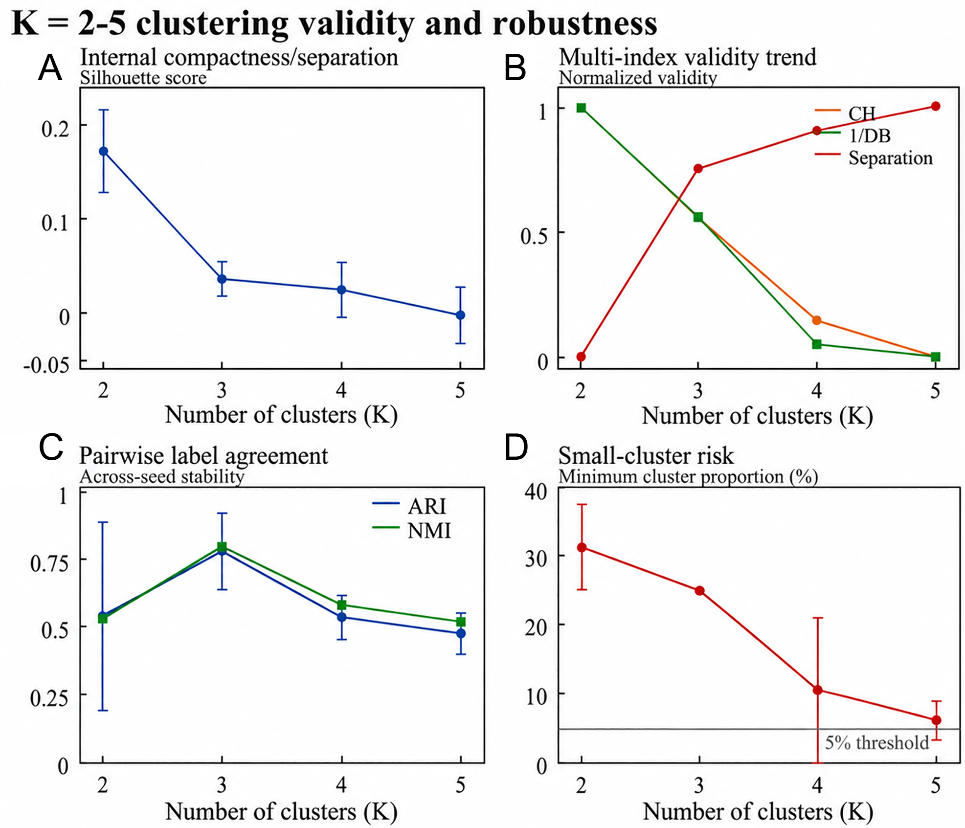
Figure 8. Validity and robustness analysis of ICG waveform clustering results under different numbers of clusters. A total of N = 1,908 valid ICG beat segments are included. (A) Silhouette score for K = 2-5. (B) Normalized trends of multiple clustering validity metrics. (C) Label consistency across random seeds. (D) Minimum cluster proportion and the 5% small-cluster risk threshold. Except for the normalized trend plot, the points represent the mean values over five repeated runs, and the error bars indicate ±1 standard deviation (mean ± SD). ARI and NMI are calculated from 10 pairwise label comparisons generated from five runs for each K value.
Internal validity, cluster-size balance, and cross-seed stability for K = 2-5 clustering
| Metric | K = 2 | K = 3 | K = 4 | K = 5 |
| Silhouette | 0.171 ± 0.044 | 0.036 ± 0.018 | 0.024 ± 0.029 | -0.003 ± 0.030 |
| Calinski-harabasz | 178.496 ± 7.221 | 138.288 ± 1.533 | 101.119 ± 5.116 | 88.190 ± 10.572 |
| Davies-bouldin | 2.701 ± 0.077 | 3.012 ± 0.016 | 3.480 ± 0.655 | 3.533 ± 0.385 |
| Separation ratio | 1.449 ± 0.050 | 1.544 ± 0.006 | 1.563 ± 0.102 | 1.575 ± 0.049 |
| Minimum-cluster proportion (%) | 31.184 ± 6.293 | 24.916 ± 0.368 | 10.440 ± 10.320 | 6.059 ± 2.761 |
| Stability ARI | 0.538 ± 0.350 | 0.777 ± 0.145 | 0.532 ± 0.084 | 0.471 ± 0.076 |
| Stability NMI | 0.528 ± 0.247 | 0.796 ± 0.116 | 0.577 ± 0.058 | 0.514 ± 0.061 |
| Medoid DTW distance | 1,772.82 ± 45.12 | 1,549.95 ± 2.38 | 1,533.89 ± 19.28 | 1,496.79 ± 18.30 |
| Relative inertia | 1.000 | 0.874 | 0.865 | 0.844 |
| Decrease from previous K (%) | - | 12.57 | 1.04 | 2.42 |
Morphological classification results of ICG waveforms
To further validate the morphological diversity and learnability of ICG waveforms, this study performs morphology classification on the preprocessed ICG beat segments using the clustering-derived labels. For each K value, the test set contains n = 382 beat segments. In the classification tasks with K = 2, K = 3, K = 4, and K = 5, the complete MS-GBiLSTM-TA model achieves Accuracy values of 95.03%, 91.36%, 89.79%, and 76.96%, respectively. The corresponding Macro-F1 scores are 0.9432, 0.9134, 0.8507, and 0.7686, while the Weighted-F1 scores are 0.9501, 0.9135, 0.8982, and 0.7714, respectively. Detailed class-level Precision, Recall, and F1-score results are presented in Tables 2-5. As the number of clusters increases, the classification task becomes more difficult and model performance declines, indicating that finer-grained partitioning of ICG waveform morphologies leads to greater feature overlap and less distinct boundaries between classes.
Binary classification results for ICG waveforms in the HeartCycle dataset
| Class | Precision | Recall | F1 |
| 0 | 0.9344 | 0.9120 | 0.9231 |
| 1 | 0.9577 | 0.9689 | 0.9632 |
| Macro average | 0.9461 | 0.9404 | 0.9432 |
| Weighted average | 0.9501 | 0.9503 | 0.9501 |
Three-class classification results for ICG waveforms in the HeartCycle dataset
| Class | Precision | Recall | F1 |
| 0 | 0.9539 | 0.8841 | 0.9177 |
| 1 | 0.8571 | 0.9897 | 0.9187 |
| 2 | 0.9153 | 0.8926 | 0.9038 |
| Macro average | 0.9088 | 0.9221 | 0.9134 |
| Weighted average | 0.9171 | 0.9136 | 0.9135 |
Four-class classification results for ICG waveforms in the HeartCycle dataset
| Class | Precision | Recall | F1 |
| 0 | 0.9091 | 0.9091 | 0.9091 |
| 1 | 0.9030 | 0.9030 | 0.9030 |
| 2 | 0.9294 | 0.9186 | 0.9240 |
| 3 | 0.6500 | 0.6842 | 0.6667 |
| Macro average | 0.8479 | 0.8537 | 0.8507 |
| Weighted average | 0.8986 | 0.8979 | 0.8982 |
Five-class classification results for ICG waveforms in the HeartCycle dataset
| Class | Precision | Recall | F1 |
| 0 | 0.9455 | 0.8814 | 0.9123 |
| 1 | 0.6024 | 0.7353 | 0.6623 |
| 2 | 0.7143 | 0.6190 | 0.6633 |
| 3 | 0.8814 | 0.8455 | 0.8631 |
| 4 | 0.6571 | 0.8519 | 0.7419 |
| Macro average | 0.7601 | 0.7866 | 0.7686 |
| Weighted average | 0.7798 | 0.7696 | 0.7714 |
Figure 9 presents the corresponding confusion matrices. As the number of classes increases, the number of off-diagonal elements also increases, indicating more pronounced class confusion in fine-grained ICG morphology recognition. Further analysis of the class-level results reveals several difficult classes in the multiclass tasks. For example, in the four-class classification task, Class 3 achieves a Recall of 0.6842, a Precision of 0.6500, and an F1-score of 0.6667, indicating that this class remains difficult to identify accurately. This finding suggests that some ICG waveform subtypes exhibit high local morphological similarity to other classes, making it difficult for the model to learn stable and discriminative feature representations. The differences between the macro-averaged and weighted-averaged metrics further reflect the influence of class imbalance on performance evaluation. When minority classes are difficult to identify, the macro-averaged metrics decrease more markedly, indicating that the model does not perform uniformly across classes. Overall, the morphology classification results provide data-driven support for the preceding clustering analysis, showing that ICG waveforms exhibit substantial morphological diversity and class overlap under real-beat conditions. These findings indicate that rigidly matching specific mechanical events using only local morphological features from single-modal ICG can lead to temporal ambiguity and localization drift in complex waveforms. This observation provides further motivation for incorporating ECG and PCG into the subsequent multimodal fiducial point localization framework.
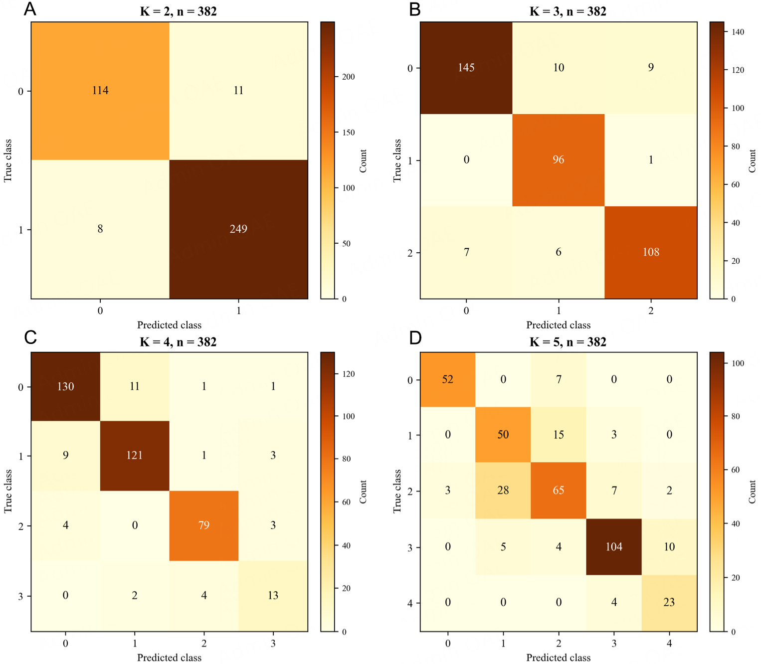
Figure 9. Confusion matrices of ICG morphology classification results under different clustering schemes in the HeartCycle dataset. All confusion matrices are generated from the test set with n = 382 beat segments, and the values in each cell represent the number of samples assigned to the corresponding category. (A) Binary classification. (B) Three-class classification. (C) Four-class classification. (D) Five-class classification.
The structural ablation experiments evaluate the contributions of multiscale convolution, bidirectional temporal modeling, and temporal attention across different ICG morphology classification tasks. All models are compared using the same training, validation, and test splits, and the test set for each K value contains
Structural ablation results of the MS-GBiLSTM-TA classification model
| K | Model | n | Accuracy | Macro-F1 | Weighted-F1 |
| 2 | CNN-only | 382 | 0.9555 | 0.9496 | 0.9555 |
| BiLSTM-only | 0.9188 | 0.9080 | 0.9189 | ||
| CNN + BiLSTM | 0.9450 | 0.9366 | 0.9446 | ||
| MS-GBiLSTM-TA | 0.9503 | 0.9432 | 0.9501 | ||
| 3 | CNN-only | 0.8665 | 0.8718 | 0.8657 | |
| BiLSTM-only | 0.9058 | 0.9072 | 0.9053 | ||
| CNN + BiLSTM | 0.8717 | 0.8711 | 0.8713 | ||
| MS-GBiLSTM-TA | 0.9136 | 0.9134 | 0.9135 | ||
| 4 | CNN-only | 0.8325 | 0.7956 | 0.8347 | |
| BiLSTM-only | 0.8927 | 0.8597 | 0.8946 | ||
| CNN + BiLSTM | 0.8848 | 0.8465 | 0.8886 | ||
| MS-GBiLSTM-TA | 0.8979 | 0.8507 | 0.8982 | ||
| 5 | CNN-only | 0.7120 | 0.6954 | 0.7161 | |
| BiLSTM-only | 0.7382 | 0.7383 | 0.7411 | ||
| CNN + BiLSTM | 0.7775 | 0.7595 | 0.7783 | ||
| MS-GBiLSTM-TA | 0.7696 | 0.7686 | 0.7714 |
ICG feature-point localization and hemodynamic parameter estimation results
The preceding clustering and classification analyses demonstrate that ICG waveforms exhibit substantial morphological variability and feature overlap. This implies that relying solely on local morphological characteristics from single-modality ICG to match specific mechanical events is prone to temporal ambiguity and localization drift, which can further propagate as cumulative errors in beat-to-beat hemodynamic parameter estimation. Therefore, single-modality local morphological analysis still faces challenges in achieving stable event localization under complex waveform conditions. Motivated by these findings, we further compared the performance of conventional rule-based methods and multimodal deep learning approaches in both key feature-point localization and downstream hemodynamic parameter estimation.
The comparative methods fall into two categories. The conventional rule-based approaches include the ECG-only method, which relies exclusively on ECG for temporal anchoring, and the ECG + PCG-assisted method, which further incorporates soft constraints derived from PCG heart sound events. The deep learning approaches include deep learning (DL) w/o PCG, which excludes PCG input, and DL + PCG, which explicitly integrates PCG into the multimodal framework. Error statistics were computed on the basis of the relative error for each valid beat and then aggregated as the MAPE for comparison. For overall reference, Table 7 summarizes the mean MAPE (%) of all methods for LVET, SV, and CO.
Comparison of mean absolute percentage error (MAPE, %) across different methods
| Methods | LVET | SV | CO |
| ECG-only | 15.45 | 14.67 | 18.35 |
| ECG +PCG-assisted | 14.84 | 13.89 | 17.50 |
| DL w/o PCG | 21.11 | 8.31 | 9.00 |
| DL + PCG | 16.04 | 6.51 | 7.35 |
To address statistical uncertainty, this study retains the beat-level mean MAPE reported in the original manuscript as the primary result and additionally reports the mean ± SD, median [IQR], and 95% CI of the error distributions for each method, as shown in Table 8. The beat-level MAPE statistics in Table 8 describe the per-beat error performance and dispersion of each method within its corresponding evaluation cohort, whereas statistical inference for between-method comparisons is conducted at the subject level.
Descriptive statistics of beat-level MAPE for different methods (%)
| Method | Metric | Number of valid beat segments | Mean ± SD | Median [IQR] | 95%CI |
| ECG-only | LVET | 92 | 15.45 ± 6.65 | 15.25 [10.88,19.01] | 14.09-16.81 |
| SV | 14.67 ± 6.74 | 14.53 [9.68, 17.53] | 13.30-16.05 | ||
| CO | 18.35 ± 8.44 | 16.62 [12.54,23.92] | 16.62-20.07 | ||
| ECG + PCG-assisted | LVET | 14.84 ± 6.75 | 14.99 [10.61,18.94] | 13.46-16.22 | |
| SV | 13.89 ± 6.52 | 13.13 [9.32, 16.28] | 12.56-15.22 | ||
| CO | 17.50 ± 7.76 | 16.42 [12.77,20.79] | 15.92-19.09 | ||
| DL w/o PCG | LVET | 61 | 21.11 ± 13.81 | 16.81 [11.21,33.23] | 17.64-24.57 |
| SV | 8.31 ± 5.10 | 7.30 [4.42,11.85] | 7.03-9.58 | ||
| CO | 9.00 ± 5.37 | 9.20 [5.65,12.59] | 7.65-10.35 | ||
| DL + PCG | LVET | 16.04 ± 8.31 | 17.56 [9.37,21.85] | 13.96-18.13 | |
| SV | 6.51 ± 4.91 | 5.95 [2.35, 9.51] | 5.28-7.75 | ||
| CO | 7.35 ± 4.56 | 6.43 [3.77,10.53] | 6.20-8.49 |
Because each subject can contribute multiple beats, individual beats are not treated as independent observations in subject-level statistical inference. The paired analysis reported in Table 9 is based on the results of 17-fold LOSO cross-validation. In each fold, one subject is completely held out as the independent test subject, one subject is used for model selection, and the remaining 15 subjects are used for model training. CH01 through CH17 serve once each as the independent test subject, and the statistical result for each subject is obtained exclusively from the fold in which that subject is completely held out. DL + PCG and DL w/o PCG use identical training, validation, and test subject assignments in every fold and are evaluated on the common test beats with complete reference values. The MAPE values for LVET, SV, and CO are first aggregated within each test subject, after which paired tests are conducted using the aggregated results from the 17 independent test subjects. For both method comparisons, ΔMAPE is calculated within each subject as the MAPE of the method without PCG minus that of the corresponding PCG-assisted method. Specifically,
Paired statistical tests based on subject-level MAPE
| Comparison | Metric | Number of subjects | ΔMAPE(%) | Paired t-test P | Wilcoxon P |
| ECG + PCG-assisted vs. ECG-only | LVET | 17 | 0.46 | 0.312 | 0.281 |
| SV | 0.78 | 0.425 | 0.463 | ||
| CO | 0.83 | 0.389 | 0.412 | ||
| DL + PCG vs. DL w/o PCG | LVET | 0.98 | 0.512 | 0.488 | |
| SV | 2.43 | 0.004 | 0.007 | ||
| CO | 2.16 | 0.028 | 0.035 |
Based on the independent test results from the 17-fold LOSO evaluation reported in Table 9, DL + PCG shows overall reductions in subject-level MAPE for SV and CO compared with DL w/o PCG, with both the paired t-test and the Wilcoxon signed-rank test indicating statistically significant differences. The ΔMAPE for LVET is also positive, although the difference does not reach statistical significance. For the conventional rule-based methods, ECG + PCG-assisted methods yield positive ΔMAPE values for LVET, SV, and CO compared with ECG-only, but none of the paired tests for these three metrics reach statistical significance. These results indicate that, under subject-independent LOSO evaluation, the mechanical-event timing information provided by PCG offers a clearer complementary contribution to SV and CO estimation within the deep learning framework, whereas the improvements observed in the conventional rule-based methods are primarily numerical trends.
Baseline performance of conventional rule-based methods and gains from PCG soft constraints
Within the conventional rule-based localization framework, the ECG-only method relies solely on ECG-derived electrical activity as a temporal anchor to constrain the search windows for the B and X points. Consequently, its performance is highly dependent on the local morphological characteristics of the ICG waveform. However, as demonstrated in the preceding clustering and classification analyses, real-world ICG signals exhibit substantial morphological variability and feature overlap, often accompanied by distortions such as double peaks, flattened incisura, and baseline drift. Under such conditions, the ECG-only method is more susceptible to local morphological ambiguities, leading to localization errors that propagate into the parameter estimation stage. As shown in Figure 10, the resulting MAPE values for LVET, SV, and CO are 15.45%, 14.67%, and 18.35%, respectively. In contrast, the ECG + PCG-assisted method incorporates mechanical event priors derived from PCG, using S1 and S2 to impose soft constraints on the candidate intervals for the B and X points. The inclusion of PCG leads to consistent, albeit modest, improvements across all three metrics: the MAPE for LVET decreases from 15.45% to 14.84%, SV from 14.67% to 13.89%, and CO from 18.35% to 17.50%. These results indicate that even within a rule-based framework, PCG-derived mechanical priors can partially mitigate temporal ambiguity caused by ICG waveform distortion and reduce gross localization errors. Overall, while incorporating PCG provides measurable performance gains, the improvements remain limited. This suggests that constraining search windows alone can reduce extreme errors to some extent, but is insufficient to fundamentally resolve the feature-point ambiguity arising from the complex and variable morphology of ICG waveforms. A direct numerical comparison of the two conventional rule-based methods is provided in Table 10.
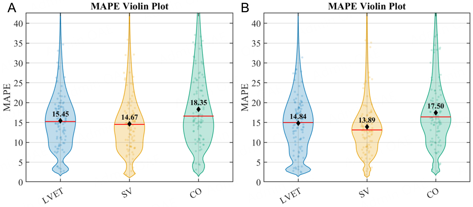
Figure 10. Beat-level MAPE distributions of the conventional rule-based method under different auxiliary information conditions. (A and B) correspond to ECG-only and ECG + PCG-assisted, respectively. Each method is evaluated on n = 92 valid test beats. Each dot represents an individual beat; the width of the half violin indicates the kernel density distribution of MAPE values, the horizontal line represents the median, and the diamond indicates the mean.
Comparison of results for conventional rule-based methods
| Methods | LVET | SV | CO |
| ECG-only | 15.45 | 14.67 | 18.35 |
| ECG + PCG-assisted | 14.84 | 13.89 | 17.50 |
Parameter estimation performance of multimodal deep learning fusion
In the deep learning framework, DL + PCG achieves relatively low errors in SV and CO estimation. As shown in Figure 11, the best-performing conventional rule-based method, ECG + PCG-assisted, is evaluated on n = 92 valid test beats, whereas DL + PCG is evaluated on n = 61 valid test beats with complete reference values for LVET, SV, and CO. Within their respective evaluable beat sets, ECG + PCG-assisted yields mean MAPE values of 13.89% for SV and 17.50% for CO, while DL + PCG yields corresponding values of 6.51% and 7.35%. These side-by-side results indicate that end-to-end multimodal modeling achieves lower SV and CO error levels under the current evaluation conditions. Because the two method categories are evaluated on different numbers of valid beats, this cross-category numerical comparison is presented descriptively rather than as a direct statistical comparison. The specific contribution of PCG to the deep learning model is further assessed in the subsequent ablation experiment using the same set of test beats.
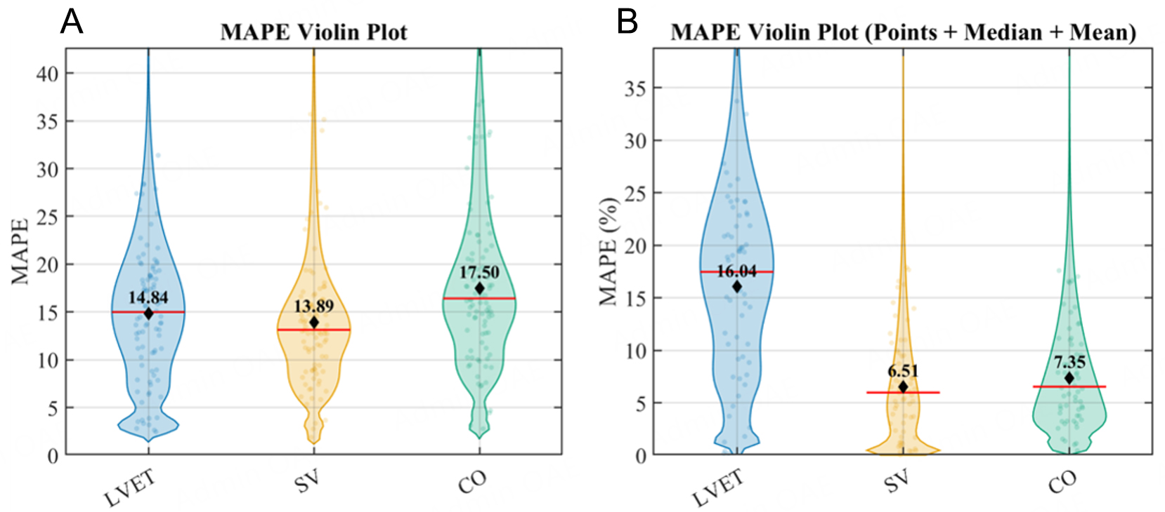
Figure 11. Beat-level MAPE distributions of the best-performing conventional method and the multimodal deep learning fusion method. (A and B) correspond to ECG + PCG-assisted (n = 92) and DL + PCG (n = 61), respectively. Each dot represents an individual valid beat; the width of the half violin indicates the kernel density distribution of MAPE values, the horizontal line represents the median, and the diamond indicates the mean.
For the deep learning models with beat-level true and predicted outputs, additional analyses were conducted using mean absolute error (MAE), root mean square error (RMSE), Pearson correlation coefficients, and Bland-Altman agreement analysis, as presented in Table 11 and Figure 12. These analyses were intended to complement the MAPE-based results from the perspectives of absolute error, linear correlation, and agreement, without changing the original presentation of beat-level mean MAPE as the primary outcome measure. The results showed that DL + PCG yielded lower absolute errors than DL w/o PCG for both SV and CO estimation, with MAEs of 7.12 ± 5.76 mL and 0.53 ± 0.36 L/min, respectively, and RMSEs of 9.13 mL and 0.64 L/min, respectively. Bland-Altman analysis showed biases of -6.71 mL for SV and -0.49 L/min for CO with DL + PCG, with corresponding 95% limits of agreement of -18.95 to 5.53 mL and -1.31 to 0.33 L/min, respectively. Pearson correlation coefficients were reported as supplementary metrics to reflect the linear correspondence between predicted and reference values across the dynamic range of the test set.
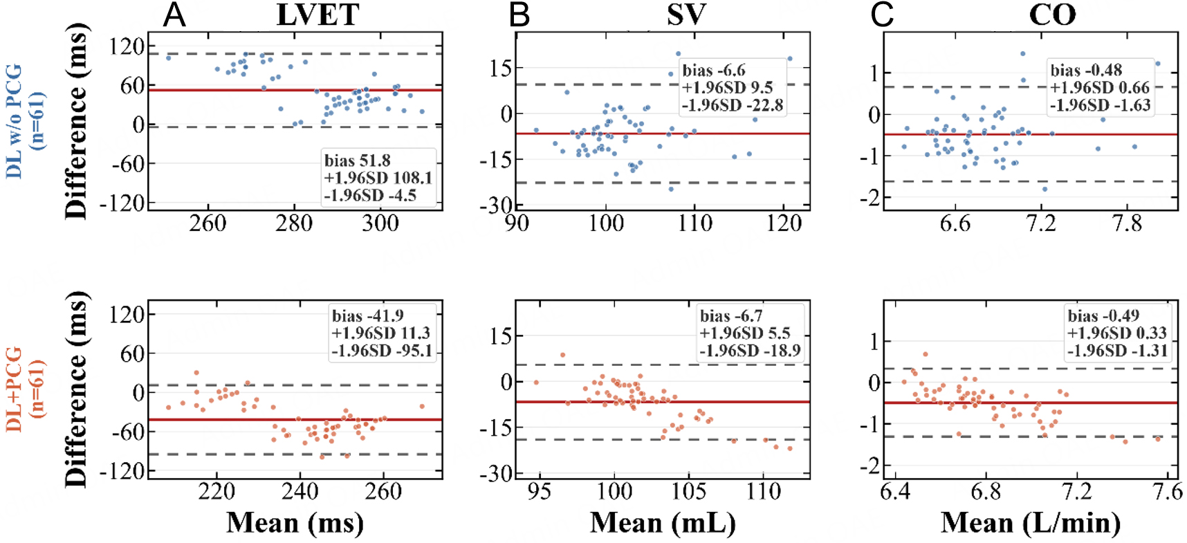
Figure 12. Bland-Altman agreement analysis of beat-level estimation results from the deep learning model (n = 61 predicted-reference pairs in each panel). (A-C) correspond to LVET, SV, and CO, respectively. The solid line represents the mean bias, and the dashed lines indicate the 95% limits of agreement.
Absolute error, correlation, and agreement analysis for beat-level predictions of the deep learning models
| Method | Metric | n | MAE ± SD | RMSE | Pearson r | Bias (95% LoA) |
| DL w/o PCG | LVET | 61 | 51.79 ± 28.73 ms | 59.12 ms | -0.080 | 51.79 (-4.52, 108.11) ms |
| SV | 61 | 8.87 ± 5.68 mL | 10.51 mL | 0.282 | -6.62 (-22.76, 9.52) mL | |
| CO | 61 | 0.64 ± 0.40 L/min | 0.75 L/min | 0.190 | -0.48 (-1.63, 0.66) L/min | |
| DL + PCG | LVET | 61 | 43.55 ± 24.39 ms | 49.81 ms | 0.088 | -41.90 (-95.13, 11.32) ms |
| SV | 61 | 7.12 ± 5.76 mL | 9.13 mL | 0.074 | -6.71 (-18.95, 5.53) mL | |
| CO | 61 | 0.53 ± 0.36 L/min | 0.64 L/min | 0.200 | -0.49 (-1.31, 0.33) L/min |
Building on these results, additional comparisons with learning-based baseline models were conducted, as shown in Table 12 and Figure 13, to exclude the possibility that the performance improvement was solely attributable to the increased capacity of a generic deep sequential model. On the same beat-level test set used in the main experiments, the CNN-only, BiLSTM, and CNN + BiLSTM baseline models were trained using identical ECG, ICG, and PCG inputs and the same signal preprocessing pipeline. Because multiple architectural differences exist between these baseline models and the Proposed model, this comparison is used to evaluate the relative performance of the complete framework rather than to quantitatively isolate the independent contribution of the event query mechanism or any individual structural component.
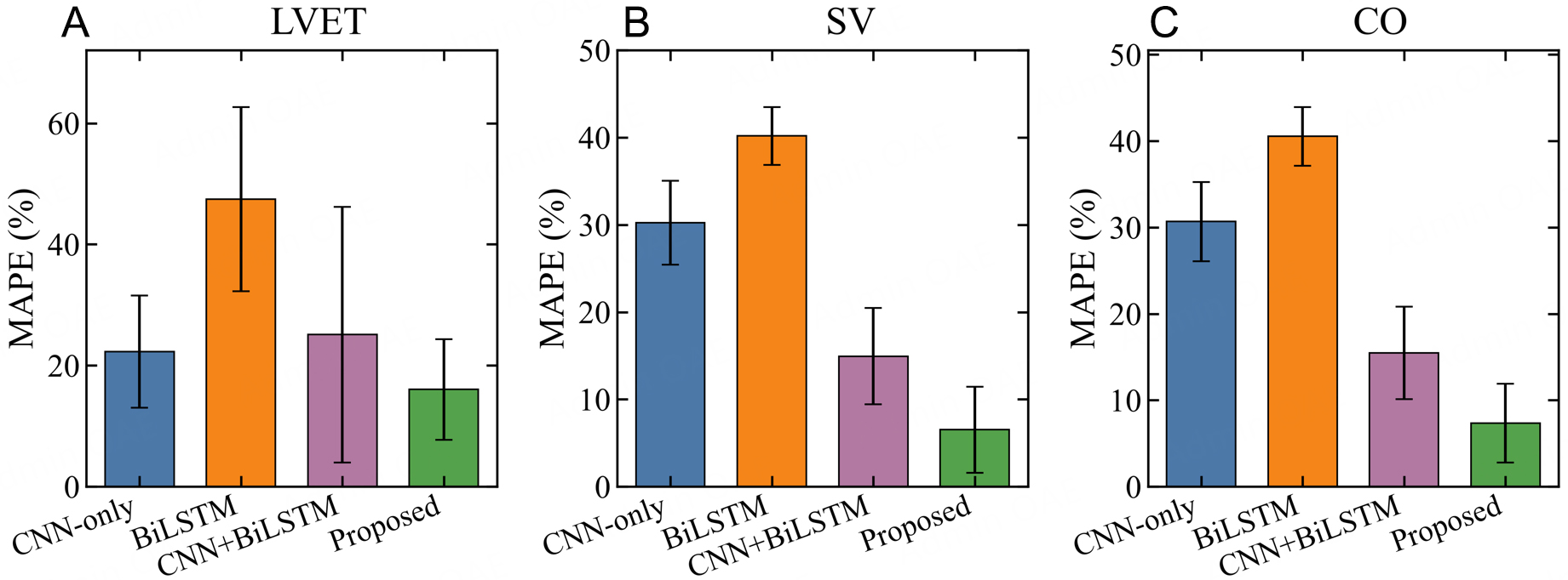
Figure 13. Comparison of MAPE values for beat-level hemodynamic parameter estimation among different learning-based models. (A-C) correspond to LVET, SV, and CO, respectively. The bar height represents the mean MAPE calculated from n = 61 valid test beats, and the error bars indicate mean ± SD.
Performance comparison of learning-based baseline models on the main beat-level test set
| Model | Metric | n | MAE | RMSE | MAPE mean ± SD (%) | Median [IQR] (%) |
| CNN-only | LVET | 61 | 59.92 | 65.97 | 22.29 ± 9.24 | 23.45 [13.87] |
| SV | 61 | 32.08 | 32.75 | 30.23 ± 4.80 | 29.93 [5.92] | |
| CO | 61 | 2.18 | 2.22 | 30.67 ± 4.57 | 29.94 [6.00] | |
| BiLSTM | LVET | 61 | 120.29 | 123.06 | 47.45 ± 15.21 | 41.98 [23.49] |
| SV | 61 | 42.55 | 42.97 | 40.17 ± 3.31 | 39.73 [4.91] | |
| CO | 61 | 2.87 | 2.90 | 40.54 ± 3.39 | 39.97 [4.27] | |
| CNN + BiLSTM | LVET | 61 | 66.29 | 86.97 | 25.08 ± 21.13 | 22.25 [24.29] |
| SV | 61 | 16.02 | 17.38 | 14.93 ± 5.52 | 13.96 [8.17] | |
| CO | 61 | 1.11 | 1.19 | 15.46 ± 5.37 | 14.53 [6.77] | |
| Proposed | LVET | 61 | 43.55 | 49.81 | 16.04 ± 8.31 | 17.56 [12.48] |
| SV | 61 | 7.12 | 9.13 | 6.51 ± 4.91 | 5.95 [7.16] | |
| CO | 61 | 0.53 | 0.64 | 7.35 ± 4.56 | 6.43 [6.77] |
The results show that, compared with the three learning-based baselines, including CNN-only, BiLSTM, and CNN + BiLSTM, the Proposed model achieves lower estimation errors for LVET, SV, and CO. Specifically, the Proposed model obtains mean MAPE values of 16.04%, 6.51%, and 7.35% for LVET, SV, and CO estimation, respectively. In comparison, the CNN-only model achieves 22.29%, 30.23%, and 30.67%, the BiLSTM model achieves 47.45%, 40.17%, and 40.54%, and the CNN + BiLSTM model achieves 25.08%, 14.93%, and 15.46%, respectively. These results indicate that relying solely on convolutional feature extraction, recurrent sequence modeling, or their combination remains insufficient for fully capturing the multimodal contextual information related to ejection events across ECG, ICG, and PCG signals. In contrast, the complete Proposed framework achieves lower parameter estimation errors under the current test set and unified input conditions. This result is consistent with the interpretation that multimodal temporal information and event-related context modeling may contribute to improved beat-level parameter estimation stability. However, since this comparison does not independently isolate the event-token mechanism, it should not be interpreted as direct evidence of the independent contribution of event-token.
To further assess the independent contribution of local morphological information from the single-channel ICG signal to fiducial-point localization and hemodynamic parameter estimation, an additional ICG-only baseline model was included, with the results presented in Table 13 and Figure 14. This model used only the single-channel ICG signal as input, without incorporating the electrical activity timing anchors provided by ECG or the valve-related mechanical event timing information provided by PCG. Apart from the input modality, the ICG-only baseline followed exactly the same data partitioning, preprocessing pipeline, number of training epochs, best-checkpoint selection strategy based on the validation set, and test-set evaluation procedure as those used in the main experiments, thereby ensuring a fair comparison across methods.
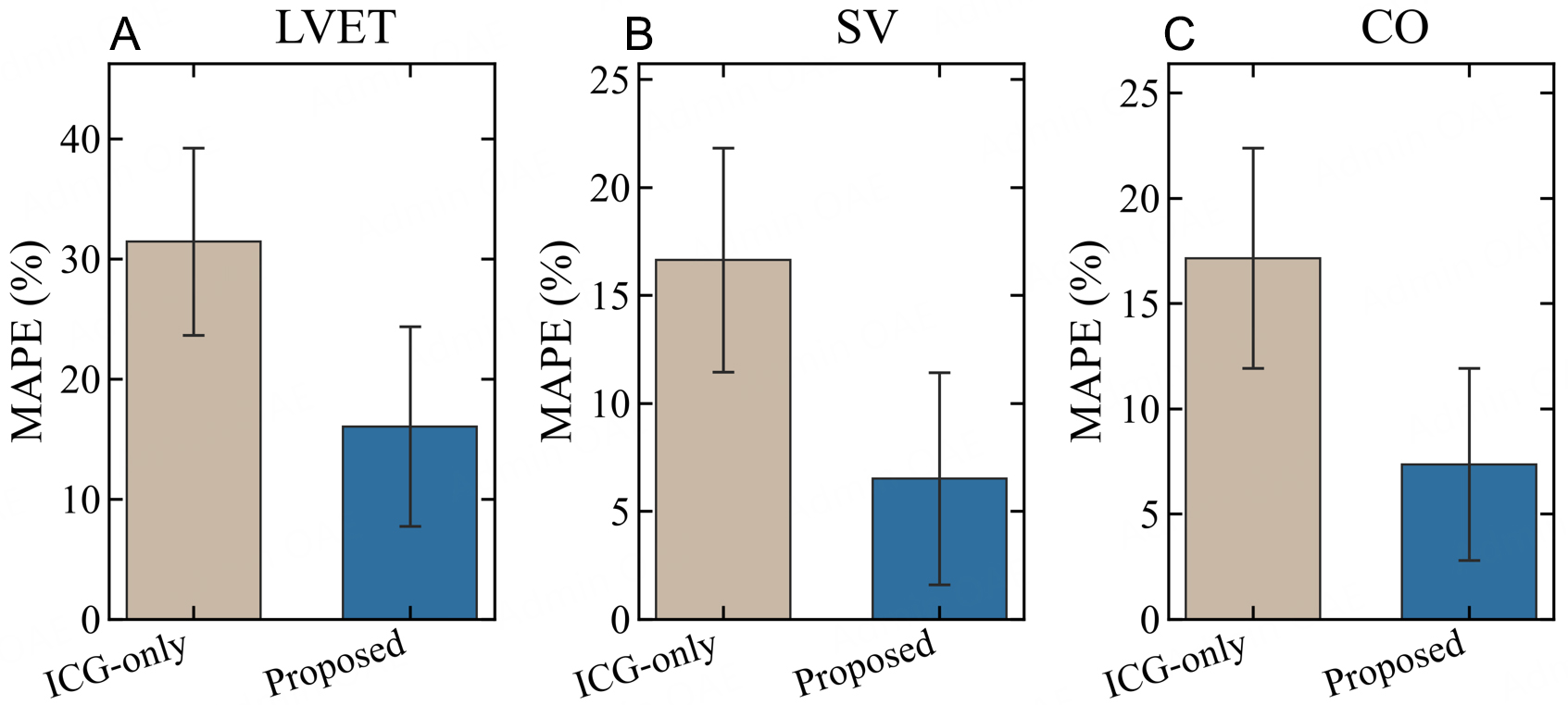
Figure 14. Comparison of MAPE values for beat-level hemodynamic parameter estimation between the single-channel ICG-only model and the proposed model. (A-C) correspond to LVET, SV, and CO, respectively. The bar height represents the mean MAPE calculated from n = 61 valid test beats, and the error bars indicate mean ± SD.
Validation of the single-channel ICG model for direct feature-point localization and parameter estimation
| Model | Metric | n | MAE | RMSE | MAPE mean ± SD (%) | Median [IQR] (%) |
| ICG-only | LVET | 61 | 83.79 | 87.81 | 31.41 ± 7.80 | 34.85 [11.41] |
| SV | 61 | 17.79 | 18.86 | 16.63 ± 5.18 | 16.29 [6.81] | |
| CO | 61 | 1.23 | 1.30 | 17.15 ± 5.23 | 17.60 [5.72] | |
| Proposed | LVET | 61 | 43.55 | 49.81 | 16.04 ± 8.31 | 17.56 [12.48] |
| SV | 61 | 7.12 | 9.13 | 6.51 ± 4.91 | 5.95 [7.16] | |
| CO | 61 | 0.53 | 0.64 | 7.35 ± 4.56 | 6.43 [6.77] |
The results showed that the ICG-only model achieved mean MAPEs of 31.41%, 16.63%, and 17.15% for LVET, SV, and CO, respectively, all of which were higher than the corresponding values of 16.04%, 6.51%, and 7.35% obtained by the proposed model. These findings suggest that reliance on local morphology from a single ICG channel alone is insufficient for stable identification of key events associated with AVO and closure, thereby limiting the accuracy of subsequent LVET, SV, and CO estimation. In contrast, the complete proposed multimodal framework achieves lower parameter estimation errors on the current test set, as shown in Table 14. This result is consistent with the interpretation that ECG-derived electrical timing anchors and PCG-derived valvular mechanical event information may provide complementary cues for ICG fiducial point localization.
Comparison of results between the best rule-based method and the DL + PCG model
| Methods | LVET | SV | CO |
| ECG + PCG-assisted | 14.84 | 13.89 | 17.50 |
| DL + PCG | 16.04 | 6.51 | 7.35 |
Impact of PCG on the deep learning model
To further quantify the contribution of PCG within the deep learning framework, we compared two configurations: DL w/o PCG and DL + PCG. As shown in Figure 15, removing PCG leads to consistent performance degradation across all three metrics: the mean MAPE of LVET increases from 16.04% to 21.11%, SV from 6.51% to 8.31%, and CO from 7.35% to 9.00%. This result suggests that the valvular mechanical event-related temporal information contained in the PCG envelope can serve as complementary input for multimodal modeling and is consistent with the reduced parameter estimation errors observed under the current evaluation conditions, highlighting the potential value of PCG information for ICG-based parameter estimation tasks.
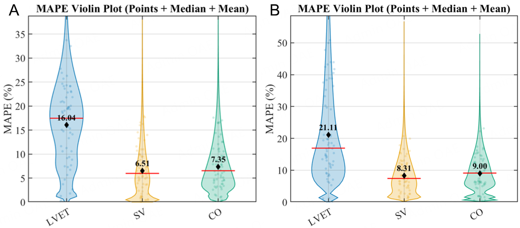
Figure 15. Effect of PCG information on the beat-level parameter estimation performance of the deep learning model. (A and B) correspond to DL + PCG and DL w/o PCG, respectively. Each configuration is evaluated on n = 61 valid test beats. Each dot represents an individual beat; the width of the half violin indicates the kernel density distribution of MAPE values, the horizontal line represents the median, and the diamond indicates the mean.
From a mechanistic perspective, the PCG envelope contains temporal information related to valvular mechanical events and can provide complementary mechanical references for ICG morphological features. Under the current data partitioning and model configuration, removing PCG results in increased estimation errors for LVET, SV, and CO. Correspondingly, the deep learning model integrating PCG achieves lower errors across all three metrics, with more pronounced improvements observed in SV and CO estimation. This ablation result indicates that PCG integration contributes to improved beat-level hemodynamic parameter estimation performance within the current complete model architecture and evaluation conditions. In the descriptive comparison of the four methods, the mean MAPE values for SV are 14.67%, 13.89%, 8.31%, and 6.51%, respectively, while those for CO are 18.35%, 17.50%, 9.00%, and 7.35%, respectively. Both metrics show an overall decreasing trend across the four configurations. LVET does not follow the same monotonic pattern, with mean MAPE values of 15.45%, 14.84%, 21.11%, and 16.04%, respectively. Nevertheless, within the conventional rule-based comparison and the deep learning comparison, the incorporation of PCG reduces the LVET error in both cases. Therefore, the current findings support the performance benefits of the complete multimodal framework and PCG integration under the conditions of this study, but they do not allow the observed improvements to be fully attributed to the event query mechanism or provide direct evidence that improved AVO/AVC localization is the primary cause of reduced downstream parameter estimation errors.
To more clearly illustrate the performance gains introduced by multimodal fusion, Figure 16 presents a heatmap of overall errors across all experimental settings. Compared with the darker regions corresponding to higher errors in conventional methods, the DL + PCG approach exhibits prominent bright regions - indicating lower errors - particularly for SV and CO. This visual contrast highlights the performance transition from rule-based matching to end-to-end feature learning.
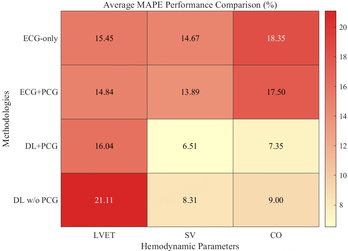
Figure 16. Heatmap of mean MAPE values for LVET, SV, and CO across the four experimental groups. Statistics for the conventional rule-based methods are based on n = 92 valid test beats, whereas statistics for the deep learning methods are based on n = 61 valid test beats. Color indicates the mean MAPE (%) of each method for the corresponding metric.
Placing the four methods within a common coordinate system provides a more intuitive view of the combined contributions of PCG information and deep learning-based modeling. Figures 17 and 18 present the results of the four methods from the perspectives of error distributions and metric-specific performance, respectively. Because the conventional rule-based and deep learning methods are evaluated on n = 92 and
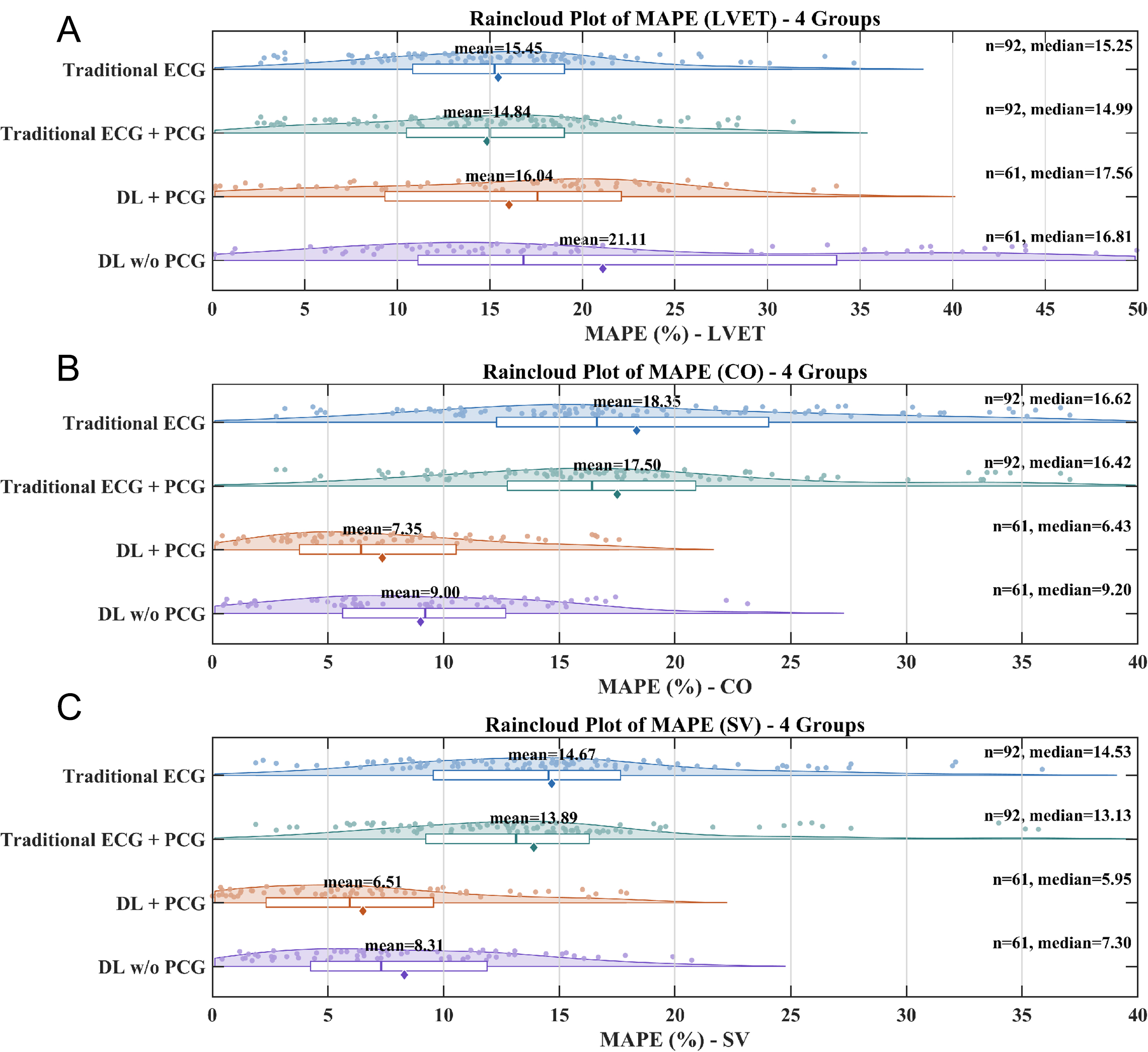
Figure 17. Raincloud plots of beat-level MAPE for LVET, SV, and CO across four methods. (A) Beat-level MAPE distribution for LVET. (B) Beat-level MAPE distribution for CO. (C) Beat-level MAPE distribution for SV. The conventional rule-based methods, ECG-only and ECG + PCG-assisted, are each evaluated on n = 92 valid test beats, whereas the deep learning methods, DL w/o PCG and DL + PCG, are each evaluated on n = 61 valid test beats. The scatter points represent the MAPE of individual valid beats, the density curves represent the error distributions, the boxplots indicate the median and interquartile range, and the diamonds denote the mean.
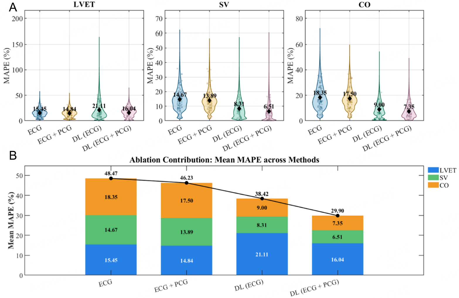
Figure 18. Analysis of metric-wise MAPE distributions and mean error composition for different methods. (A) Violin plots show the beat-level MAPE distributions. (B) Stacked bar charts show the mean MAPE composition of LVET, SV, and CO for each method. Each colored segment represents the mean MAPE of one individual metric. The total value shown above each stacked bar is the sum of the mean MAPE values for LVET, SV, and CO for the corresponding method, and the black line connects these total values across methods.
Subject-independent generalization assessed by LOSO cross-validation
To further address subject independence and model generalization, LOSO cross-validation was supplemented in this study. In each fold, one subject was completely held out as the independent test set, one subject was used as the validation set, and the remaining 15 subjects were used for model training, thereby avoiding cardiac beat segments from the same subject appearing simultaneously in the training and test sets. By iteratively treating each subject as the independent test subject, this setting provides a supplementary assessment of model generalization to unseen subjects. Unlike the fixed subject-level split used in the main experiment, LOSO cross-validation covers all 17 subjects, with each subject serving as the test subject once.
In 17-fold LOSO validation, the DL + PCG model was evaluated for beat-level LVET, SV, and CO estimation under subject-independent testing in Table 15. When summarized at the subject level, the MAPE values for LVET, SV, and CO were 21.39 ± 13.87%, 27.42 ± 21.79%, and 26.69 ± 22.39%, respectively, with 95% confidence intervals of 14.26-28.52%, 16.22-38.63%, and and15.18-38.20%. These results indicate that the multimodal framework is feasible under strict subject-independent evaluation, while the observed inter-subject variability indicates that larger samples and more diverse populations are needed to improve and validate cross-subject generalization.
Subject-level performance of the DL + PCG model under LOSO cross-validation
| Metric | Folds | MAPE mean ± SD (%) | 95%CI (%) | Median [IQR] (%) | MAE mean ± SD | RMSE mean ± SD |
| LVET | 17 | 21.39 ± 13.87 | 14.26-28.52 | 18.79 [14.99, 24.91] | 39.80 ± 21.14 ms | 45.50 ± 21.27 ms |
| SV | 17 | 27.42 ± 21.79 | 16.22-38.63 | 22.79 [14.39, 29.96] | 19.90 ± 11.25 mL | 21.44 ± 10.81 mL |
| CO | 17 | 26.69 ± 22.39 | 15.18-38.20 | 19.18 [12.53, 31.57] | 1.34 ± 0.79 L/min | 1.46 ± 0.78 L/min |
Rationale for the fixed input window
To justify the fixed input window, the temporal distributions of AVO, AVC, and conventional ICG B/X landmarks relative to the R peak were analyzed in Table 16 and Figure 19. Across 129 HDF5 record files, 1,036 AVO and 1,069 AVC events were matched from HeartCycle, and the conventional morphology-based pipeline yielded 50 B points and 50 X points. AVC, B, and X all fell within the fixed window from 0.20 s before to 0.80 s after the R peak, with 100% coverage. AVO coverage was 99.52%, and its 99% distribution range was approximately 5.30-781.44 ms, still within the upper boundary of the window. Only five AVO events were outside the window, possibly due to boundary beats, event-matching errors, or rare extreme timing. These results support the use of a fixed 1.00 s R-peak-aligned window for beat-level modeling, while also indicating that atypical timing patterns may require further consideration in broader populations.
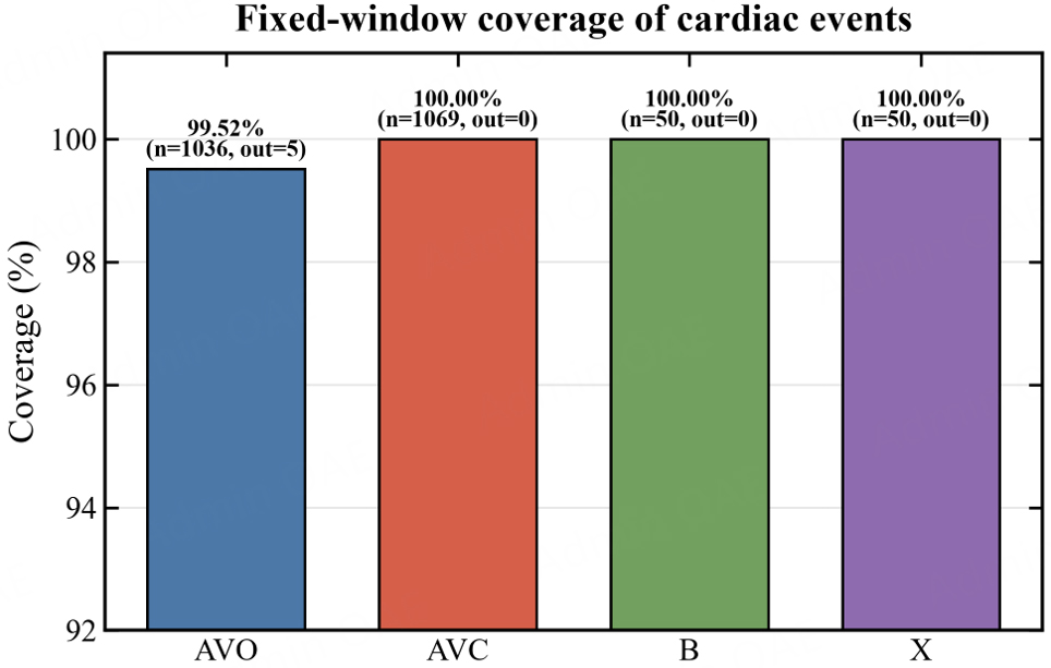
Figure 19. Coverage of AVO, AVC, and B/X events within the fixed temporal window. The sample sizes are n = 1,036 for AVO, n = 1,069 for AVC, n = 50 for B points, and n = 50 for X points. The bars or annotated values indicate the proportion of events falling within the fixed time window from 0.20 s before to 0.80 s after the R peak.
Temporal distribution and coverage of events relative to the R peak within the fixed input window
| Event | Source | n | Mean ± SD (ms) | Median [IQR] (ms) | 95% range (ms) | 99% range (ms) | Window coverage (missing n) |
| AVO | HeartCycle | 1,036 | 86.38 ± 98.81 | 74.49 [51.11] | 15.07-192.54 | 5.30-781.44 | 99.52% (5) |
| AVC | HeartCycle | 1,069 | 271.84 ± 50.47 | 272.24 [66.97] | 177.42-370.11 | 118.52-427.44 | 100.00% (0) |
| B | Rule-based B | 50 | 57.99 ± 20.76 | 60.44 [40.27] | 30.22-90.62 | 30.21-90.64 | 100.00% (0) |
| X | Rule-based X | 50 | 353.11 ± 3.94 | 352.50 [4.65] | 347.44-361.77 | 347.21-361.77 | 100.00% (0) |
From the perspective of model generalization, the advantage of the fixed-window strategy is that it provides a unified input length and a clear R-peak-aligned reference, facilitating fusion of ECG, ICG, and PCG signals on the same time axis. At the same time, the 0.20 s window before the R peak preserves local baseline and early morphological information, whereas the 0.80 s window after the R peak covers major events such as AVO, AVC, the B point, and the X point. It should be noted that this strategy also has potential limitations. Under extreme heart rates, R-peak misdetection, event-label shifts, or severe signal drift, a small number of events may approach the window boundary or even fall outside the fixed window. In addition, because the fixed window is aligned only to the R peak and no time-scale normalization is performed according to the R-R interval, the model retains true event-delay differences across beats. However, this may also increase the difficulty of model learning under marked heart-rate variability. Therefore, the window setting adopted in this study is reasonable under the current HeartCycle data distribution, but future external validation should further assess its applicability in broader heart-rate ranges and pathological populations.
DISCUSSION
This study establishes a research framework ranging from ICG waveform morphology analysis to multimodal feature fusion of ECG, ICG, and PCG to address the susceptibility of ICG fiducial point localization to waveform morphological variability in continuous noninvasive hemodynamic assessment. Clustering and classification analyses based on the HeartCycle dataset demonstrate pronounced morphological diversity, class overlap, and ambiguous boundaries among real-world ICG beats, indicating that relying solely on local morphological rules of ICG signals for B/X point localization remains challenging under complex waveform conditions. To address this issue, this study introduces ECG as an electrical timing anchor, utilizes the PCG envelope as complementary temporal information associated with valvular mechanical events, and integrates deep temporal modeling with an event query mechanism for beat-level LVET, SV, and CO estimation. Experimental results show that the complete multimodal framework achieves lower parameter estimation errors under the current evaluation conditions, with particularly improved stability in SV and CO estimation, indicating that multimodal temporal information fusion provides a feasible modeling strategy for alleviating morphological ambiguity in single-modality ICG analysis. It should be noted that the AVO, AVC, SV, and CO reference labels and values used in this study are obtained from publicly available HeartCycle HDF5 fields. Therefore, model evaluation remains affected by the reliability of the original event timestamps and hemodynamic reference values. Since the public dataset does not provide further information regarding beat-level annotation uncertainty, inter-annotator agreement, or repeated annotation variability, temporal resolution of event annotations, synchronization errors among devices, differences in event boundary determination, and resampling procedures may contribute to residual errors. Accordingly, the event fields provided by the public dataset are described as reference labels rather than error-free ground truth, and uncertainty in labels and reference values is considered an important factor affecting model performance interpretation.
Further analysis shows that compared with the model without PCG, integrating PCG reduces SV and CO estimation errors, suggesting that the PCG envelope may provide complementary mechanical information associated with ejection event timing. This finding is consistent with the interpretation that multimodal temporal information, PCG-based mechanical event context, and event query-based localization design may jointly contribute to improved beat-level parameter estimation stability. Meanwhile, the current experiments mainly evaluate the overall performance of the complete multimodal framework under unified data partitioning and evaluation procedures. The independent contribution of the event-query mechanism and the error propagation relationship between AVO/AVC localization errors and SV/CO estimation errors require further quantification through more fine-grained component ablation and error association analyses. From a practical application perspective, the results of this study support the feasibility of the proposed method for beat-to-beat hemodynamic parameter estimation under the current evaluation conditions and provide a methodological foundation for future continuous noninvasive hemodynamic trend assessment.
However, the findings of this study are primarily based on the HeartCycle public dataset and its current data distribution. Although the dataset contains multiple valid beats, and this study employs subject-level aggregated paired comparisons together with supplementary LOSO validation to strengthen the preliminary assessment of cross-subject applicability, the limited number of subjects and the single data source indicate that the current conclusions are most applicable to beat-level parameter estimation within this cohort. Future studies should further evaluate the external applicability of the model across different devices, acquisition conditions, patient populations, and multicenter cohorts. In addition, the reference values for AVO, AVC, SV, and CO are obtained from fields provided in the public dataset, and uncertainties in annotation accuracy and multimodal device synchronization may contribute to the observed errors. The available data also mainly support the evaluation of beat-level estimation performance. Incorporating controlled hemodynamic changes and long-term follow-up data in future work would facilitate further assessment of the model for continuous trend monitoring, within-subject change tracking, and analysis of the contributions of individual model components.
Conclusion
This study establishes a comprehensive framework for ICG fiducial point localization and hemodynamic parameter estimation, covering waveform morphology analysis and multimodal deep fusion modeling. Clustering and classification analyses based on the HeartCycle dataset demonstrate pronounced morphological diversity, class overlap, and ambiguous boundaries among ICG waveforms under real beat conditions, suggesting that relying solely on local morphological rules from single-modality signals for B/X point localization remains limited under complex waveform conditions. Based on these findings, this study proposes an end-to-end deep learning model integrating ECG, ICG, and PCG and compares it with conventional rule-based methods and learning-based baseline models under a unified parameter derivation and evaluation framework. Experimental results demonstrate that the proposed multimodal framework can achieve beat-level LVET, SV, and CO estimation under the current evaluation conditions, with lower errors particularly observed in SV and CO estimation. The ablation experiments and baseline comparisons are consistent with the interpretation that PCG-based mechanical event context, multimodal temporal information, and event-related modeling may jointly contribute to improved parameter estimation stability, highlighting the potential of multimodal information fusion for ICG fiducial point localization and hemodynamic parameter estimation. Further LOSO validation demonstrates the feasibility of the framework for beat-level LVET, SV, and CO estimation under subject-independent testing conditions, providing experimental support for future studies involving larger cohorts, multicenter datasets, and subject-adaptive modeling. Overall, the current results primarily support the capability of the proposed method for beat-to-beat hemodynamic parameter estimation under the evaluated conditions and provide a methodological foundation for continuous noninvasive hemodynamic trend assessment. Reliable continuous trend monitoring and within-subject tracking of hemodynamic changes require further establishment through longitudinal data, dynamic physiological scenarios, and prospective studies. Future work will incorporate independent external datasets, multicenter validation, controlled hemodynamic state variation experiments, and fine-grained structural ablation analyses to systematically evaluate the model’s external generalization capability, within-subject change tracking ability, component contributions, and clinical applicability.
DECLARATIONS
Authors’ contributions
Contributed to the study conception and design, data analysis and interpretation, and writing the manuscript: Ma S, Wang H, Cao F
Performed data acquisition and provided administrative, technical, and material support: Xu Z, Yan Z, Zhao Z
Contributed to manuscript revision and result interpretation during the revision: Wu N
Commented on the research design, data analysis, and supervision of the study: Wang H, Cao F
All authors reviewed the manuscript and approved the submitted version.
Availability of data and materials
The data used in this study were obtained from the publicly available HeartCycle dataset, HeartCycle: A comprehensive dataset of synchronized ICG and echocardiography for accurate hemodynamic predictions (version 1.0.0), hosted on PhysioNet (https://physionet.org/content/heartcycle/1.0.0/). The dataset can be accessed through PhysioNet under the Open Data Commons Attribution License v1.0. No new clinical dataset was generated in this study. The HeartCycle dataset contains synchronized ICG, ECG, echocardiography, photoplethysmography, and heart sound recordings, together with related hemodynamic and physiological parameters. The processed data and analysis scripts generated during the current study are available from the corresponding author upon reasonable request.
AI and AI-assisted tools statement
Not applicable.
Financial support and sponsorship
None.
Conflicts of interest
Cao F is an Associate Editor of The Journal of Cardiovascular Aging. Cao F is also the Guest Editor of the special issue entitled “Artificial Intelligence in Cardiovascular Aging and Disease” in The Journal of Cardiovascular Aging. Cao F was not involved in any steps of editorial processing, notably including reviewers’ selection, manuscript handling, and decision making, while the other authors have declared that they have no conflicts of interest.
Ethical approval and consent to participate
This study involved a secondary analysis of the publicly available and de-identified HeartCycle v1.0.0 dataset. The original HeartCycle study was approved by the Ethics Committee of the University of Coimbra Hospital (reference CES-238) and was conducted in accordance with the Declaration of Helsinki. Written informed consent was obtained from all participants before data collection. No new participants were recruited, and no identifiable personal information was accessed in the present study.
Consent for publication
Not applicable.
Copyright
© The Author(s) 2026.
REFERENCES
1. Kubicek WG, Patterson RP, Witsoe DA. Impedance cardiography as a noninvasive method of monitoring cardiac function and other parameters of the cardiovascular system. Ann N Y Acad Sci. 2006;170:724-32.
2. Lababidi Z, Ehmke DA, Durnin RE, Leaverton PE, Lauer RM. The first derivative thoracic impedance cardiogram. Circulation. 1970;41:651-8.
3. Sherwood(chair) A, Allen MT, Fahrenberg J, Kelsey RM, Lovallo WR, Van Doornen LJ. Methodological guidelines for impedance cardiography. Psychophysiology. 2007;27:1-23.
4. Scholte NTB, Van Ravensberg AE, Shakoor A, et al. A scoping review on advancements in noninvasive wearable technology for heart failure management. NPJ Digit Med. 2024;7:279.
5. Petek BJ, Al-Alusi MA, Moulson N, et al. Consumer wearable health and fitness technology in cardiovascular medicine: JACC state-of-the-art review. J Am Coll Cardiol. 2023;82:245-64.
6. Jamieson A, Chico TJA, Jones S, Chaturvedi N, Hughes AD, Orini M. A guide to consumer-grade wearables in cardiovascular clinical care and population health for non-experts. NPJ Cardiovasc Health. 2025;2:44.
7. Bernstein DP. Impedance cardiography: pulsatile blood flow and the biophysical and electrodynamic basis for the stroke volume equations. J Electr Bioimpedance. 2009;1:2-17.
8. Árbol JR, Perakakis P, Garrido A, Mata JL, Fernández-Santaella MC, Vila J. Mathematical detection of aortic valve opening (B point) in impedance cardiography: A comparison of three popular algorithms. Psychophysiology. 2016;54:350-7.
9. Trybek P, Sobotnicka E, Wawrzkiewicz-Jałowiecka A, et al. A new method of identifying characteristic points in the impedance cardiography signal based on empirical mode decomposition. Sensors. 2023;23:675.
10. Pan J, Tompkins WJ. A real-time QRS detection algorithm. IEEE Trans Biomed Eng. 1985;BME-32:230-6.
11. Fuller HD. Evaluation of left ventricular function by impedance cardiography: a review. Prog Cardiovasc Dis. 1994;36:267-73.
12. Karpiel I, Richter-Laskowska M, Feige D, Gacek A, Sobotnicki A. An effective method of detecting characteristic points of impedance cardiogram verified in the clinical pilot study. Sensors. 2022;22:9872.
13. Xie Y, Yu H, Xie Q. Motion impedance cardiography denoising method based on canonical correlation analysis and coherence analysis. Biomed Signal Process Control. 2023;86:105300.
14. Li X, Ni R, Ji Z. ICG signal denoising based on ICEEMDAN and PSO-VMD methods. Phys Eng Sci Med. 2024;47:1547-56.
15. Colominas MA, Schlotthauer G, Torres ME. Improved complete ensemble EMD: a suitable tool for biomedical signal processing. Biomed Signal Process Control. 2014;14:19-29.
16. Dragomiretskiy K, Zosso D. Variational mode decomposition. IEEE Trans Signal Process. 2014;62:531-44.
17. Kumari PD, Singh KM, Mayaluri ZL, et al. A hybrid variational mode decomposition framework for enhanced cardiac output estimation using impedance cardiography. Sci Rep. 2025;15:25784.
18. Pale U, Muller N, Arza A, Atienza D. ReBeatICG: real-time low-complexity beat-to-beat impedance cardiogram delineation algorithm. In 2021 43rd Annual International Conference of the IEEE Engineering in Medicine & Biology Society (EMBC); 2021 Nov 1-5; Mexico. IEEE; 2021. pp. 5618-24.
19. Inan OT, Migeotte P, Park K, et al. Ballistocardiography and seismocardiography: a review of recent advances. IEEE J Biomed Health Inform. 2015;19:1414-27.
20. Bhattacharya S, Santucci F, Jankovic M, et al. Cardiac time intervals under motion using bimodal chest E-tattoos and multistage processing. IEEE Trans Biomed Eng. 2025;72:413-24.
21. Lin DJ, Kimball JP, Zia J, Ganti VG, Inan OT. Reducing the impact of external vibrations on fiducial point detection in seismocardiogram signals. IEEE Trans Biomed Eng. 2022;69:176-85.
22. Shandhi MMH, Fan J, Heller JA, Etemadi M, Klein L, Inan OT. Estimation of changes in intracardiac hemodynamics using wearable seismocardiography and machine learning in patients with heart failure: a feasibility study. IEEE Trans Biomed Eng. 2022;69:2443-55.
23. Zhou Z, Huang J, Li H, et al. Camera seismocardiogram based monitoring of left ventricular ejection time. IEEE Trans Biomed Eng. 2025;72:2609-22.
24. Jiménez-González A. Timing the opening and closure of the aortic valve using a phonocardiogram envelope: a performance test for systolic time intervals measurement. Physiol Meas. 2021;42:025004.
25. Zang J, An Q, Li B, Zhang Z, Gao L, Xue C. A novel wearable device integrating ECG and PCG for cardiac health monitoring. Microsyst Nanoeng. 2025;11:7.
26. Illueca Fernandez E, Couceiro R, Abtahi F, et al. HeartCycle: a comprehensive dataset of synchronized impedance cardiography and echocardiography for accurate hemodynamic predictions (version 1.0.0). PhysioNet. 2025.
27. Savitzky A, Golay MJE. Smoothing and differentiation of data by simplified least squares procedures. Anal Chem. 2002;36:1627-39.
28. Mondal A, Bhattacharya P, Saha G. An automated tool for localization of heart sound components S1, S2, S3 and S4 in pulmonary sounds using Hilbert transform and Heron’s formula. SpringerPlus. 2013;2:512.
29. Thalmayer A, Zeising S, Fischer G, Kirchner J. A robust and real-time capable envelope-based algorithm for heart sound classification: validation under different physiological conditions. Sensors. 2020;20:972.
30. Sakoe H, Chiba S. Dynamic programming algorithm optimization for spoken word recognition. IEEE Trans Acoust Speech Signal Process. 1978;26:43-9.
Cite This Article
 Open Access
How to Cite
Download Citation
Export Citation File:
Type of Import
Tips on Downloading Citation
Citation Manager File Format
Type of Import
Direct Import: When the Direct Import option is selected (the default state), a dialogue box will give you the option to Save or Open the downloaded citation data. Choosing Open will either launch your citation manager or give you a choice of applications with which to use the metadata. The Save option saves the file locally for later use.
Indirect Import: When the Indirect Import option is selected, the metadata is displayed and may be copied and pasted as needed.
About This Article
Special Topic
Copyright

Data & Comments
Data
0










Comments
Comments must be written in English. Spam, offensive content, impersonation, and private information will not be permitted. If any comment is reported and identified as inappropriate content by OAE staff, the comment will be removed without notice. If you have any queries or need any help, please contact us at [email protected].