

Download PDF
Research Article  |  Open Access  |  30 Jul 2026

Kriging-based resilience assessment of low-altitude logistics networks under multiple operational disturbances

Views: 75 |  Downloads: 9 |  Cited:  0
Complex Eng. Syst. 2026, 6, 14.
10.20517/ces.2026.10 |  © The Author(s) 2026.
Author Information
Article Notes
Cite This Article

Abstract

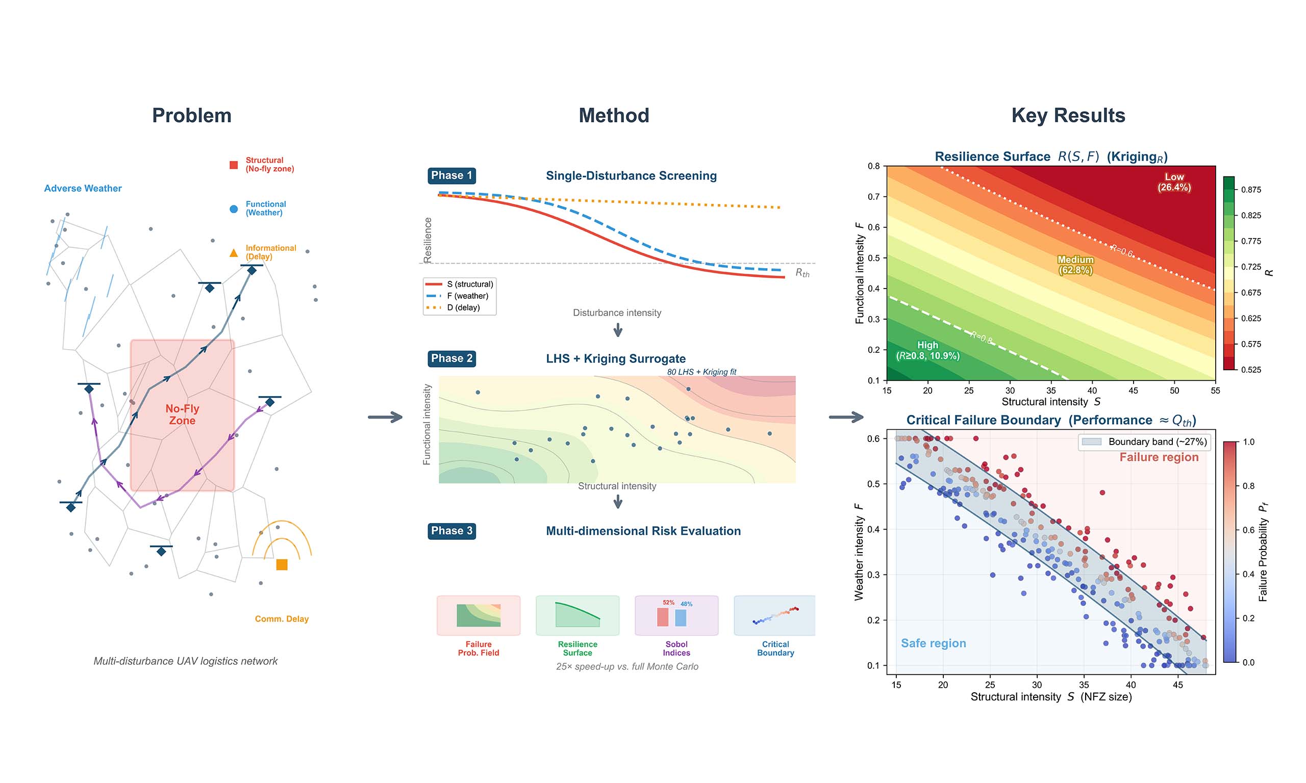
Low-altitude unmanned aerial vehicle (UAV) logistics networks are subject to multiple operational disturbances that can severely degrade delivery performance. This paper proposes a Kriging-based resilience assessment framework that efficiently evaluates the reliability and resilience of such networks under multi-dimensional disturbances. A discrete-event simulation environment is developed that incorporates Voronoi-based airspace topology, A* path planning, and dynamic re-planning. Three disturbance types—structural (no-fly zones), functional (adverse weather), and informational (communication delays)—are modelled and screened via Sobol sensitivity analysis. Two complementary Kriging surrogates, trained on Latin Hypercube samples, replace expensive Monte Carlo simulations with a 25-fold speed-up: one predicting endpoint cumulative orders for failure probability estimation, and the other predicting the integral resilience triangle index for resilience surface characterisation. Results show that structural disruption and weather degradation contribute nearly equally to performance variance (52.4% vs. 47.6%). The resilience surface reveals that only 10.9% of the disturbance parameter space sustains high resilience (R ≥ 0.8), while 26.4% falls into a low-resilience regime (R < 0.6) where severe throughput loss and incomplete recovery coexist. The proposed framework provides a computationally efficient tool for resilience-informed management of low-altitude logistics networks.
Keywords

Intelligent transportation systems, low-altitude logistics network, re-silience assessment, kriging surrogate model, failure probability mapping

1. INTRODUCTION

The rapid proliferation of unmanned aerial vehicles (UAVs) has opened a new paradigm in last-mile logistics. Urban air mobility and low-altitude delivery services promise reduced surface congestion, faster delivery times, and access to areas difficult to reach by ground transport. Major industry players and governmental agencies worldwide have invested heavily in UAV traffic management (UTM) systems, airspace integration protocols, and fleet-scale operational frameworks[1,2]. As these networks scale from pilot projects to city-wide deployments, their exposure to operational disturbances increases correspondingly.

In practice, low-altitude logistics networks face three principal categories of disruption. Structural disturbances arise when temporary no-fly zones (NFZs), imposed for security, emergency, or regulatory reasons, block portions of the airspace and force re-routing[3]. Functional disturbances stem from adverse weather conditions (wind, rain, reduced visibility) that lower achievable flight speeds and increase energy consumption[4]. Informational disturbances occur when communication links between UAVs and the UTM system experience latency or disruption, impairing dispatching and re-planning decisions[5]. In real-world operations, these disturbances frequently co-occur and interact, making isolated analysis insufficient.

Resilience—the ability of a system to absorb, adapt to, and recover from disturbances while maintaining acceptable performance—has emerged as a central concept in critical infrastructure assessment[6,7]. In the transportation domain, resilience metrics such as the resilience triangle, recovery time, and adaptive capacity have been proposed for road, rail, and air traffic systems[8,9]. For UAV systems specifically, recent work has examined resilience to individual failure modes—such as vehicle loss, communication failure, or geofence violations—but comprehensive assessments of multi-disturbance resilience remain limited[10].

Classical path planning algorithms for UAV delivery, including A*-based, metaheuristic, and stochastic optimisation methods, have been extensively studied[11,12]. At the low-altitude network level, Li et al. developed a traffic management and resource allocation framework for UAV-based parcel delivery in urban low-altitude space, integrating obstacle-aware path planning, conflict detection and resolution, and airspace allocation[13]. Recent review papers summarised drone routing, charging, security, delivery modes, and system-level design challenges, and have emphasised scalability, uncertainty handling, and real-world deployment as persistent bottlenecks[14,15,16,17].

More recently, learning-based dispatching and scheduling have emerged as an active direction in low-altitude logistics and adjacent truck–drone/courier–drone systems. In the single-vehicle domain, representative examples include DeliverSense for delivery-drone scheduling[18] and reinforcement-learning approaches for truck–drone coordinated delivery[19,20]. At the fleet level, C-SPPO addresses large-scale dynamic logistics UAV routing[21], while risk-aware multi-agent reinforcement learning has been applied to real-time courier–drone coordination in on-demand food delivery[22,23]. Most directly related to the present study, Rumman et al. proposed intelligent drone pickup scheduling via deep reinforcement learning (DRL) in low-altitude economy networks, demonstrating the promise of policy learning for pickup, delivery, and on-demand service coordination[24].

These studies apply DRL to adaptive dispatching, pickup coordination, and routing. However, their primary objective is usually to optimise service efficiency, routing cost, or delivery timeliness under nominal or scenario-specific conditions. They seldom quantify how a UAV logistics network degrades and recovers under coupled structural, functional, and informational disturbances. Resilience-oriented outputs such as failure probability fields, safe operating envelopes, and global sensitivity decompositions are rarely provided. The present work is therefore complementary to the intelligent scheduling literature. Rather than proposing another dispatching policy, we focus on fast resilience assessment of the network–policy system under disturbances. The resulting framework can later be used to compare greedy, anticipatory, and DRL-based schedulers under a common disturbance space.

Surrogate modelling techniques, particularly Kriging (Gaussian process regression), have proven effective in reliability engineering[25,26]. By replacing expensive simulations with fast-to-evaluate predictive models, Kriging enables efficient exploration of high-dimensional parameter spaces. Active learning strategies such as AK-MCS (Active Kriging with Monte Carlo Simulation) further refine surrogate accuracy near failure boundaries[25,27]. These methods have been applied successfully in structural reliability and system safety, but their use in the operational resilience of logistics networks remains limited.

Despite the progress in both optimisation and learning-based dispatching, three research gaps remain. First, most UAV network studies treat disturbances in isolation. A unified framework that simultaneously captures structural, functional, and informational disruptions is needed. Second, a full Monte Carlo simulation of multi-dimensional disturbance scenarios is prohibitively expensive. Efficient surrogate-based approaches tailored to this problem have not been explored. Third, existing resilience metrics (e.g., single-valued indices) provide limited operational guidance. Spatial risk maps, sensitivity decompositions, and failure boundaries are needed to support real-time decision-making.

To address these gaps, this paper makes three contributions:

1. A simulation-based multi-disturbance framework for low-altitude logistics networks that integrates structural, functional, and informational disruptions within a unified discrete-event simulation environment featuring Voronoi-based topology, A* path planning, and dynamic dispatching with re-planning.

2. A Kriging surrogate model trained via Latin Hypercube sampling (LHS) that replaces extensive Monte Carlo simulations, achieving a 25-fold computational speed-up while providing both mean predictions and uncertainty estimates.

3. A multi-layer resilience analysis comprising failure probability field mapping, resilience surface characterisation, Sobol global sensitivity decomposition, and critical failure boundary identification.

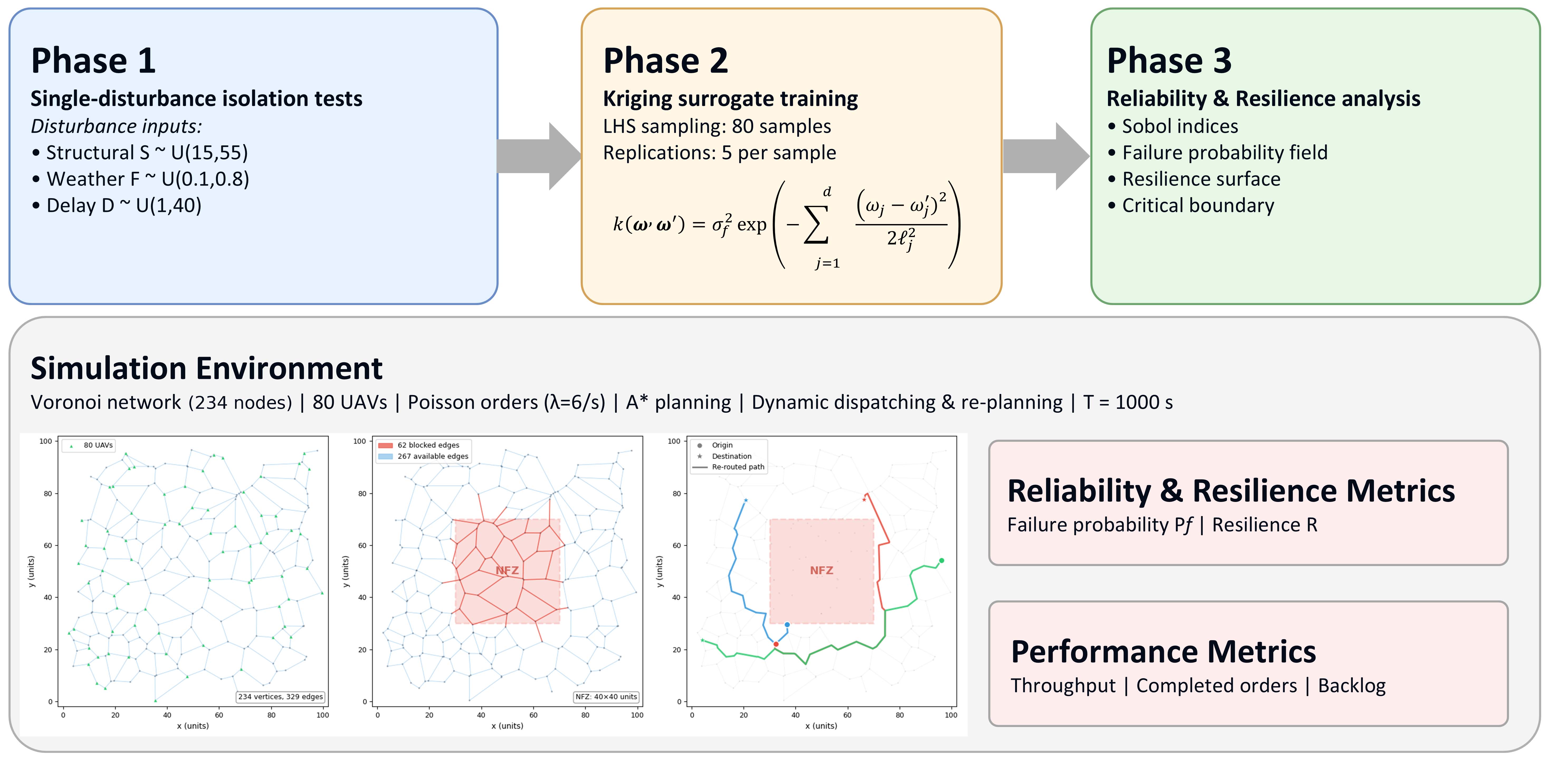
The remainder of this paper is organised as follows. Section 2 formulates the problem and presents the overall methodology. Section 3 describes the simulation environment, experimental design, and Kriging surrogate model construction. Section 4 presents and discusses the results. Section 5 concludes the paper. The overall research framework is illustrated in Figure 1.
Kriging-based resilience assessment of low-altitude logistics networks under multiple operational disturbances

Figure 1. Overall research framework. Phase 1 performs single-disturbance isolation tests. Phase 2 trains a Kriging surrogate on LHS samples. Phase 3 produces failure probability fields, resilience surfaces, Sobol indices, and the critical failure boundary.

2. PROBLEM FORMULATION AND METHODOLOGY

2.1 Low-altitude logistics network description

We consider a low-altitude UAV logistics network operating in a two-dimensional airspace. The network is modelled as an undirected graph $$ G = (V, E) $$, where $$ V $$ is the set of waypoints (vertices) and $$ E $$ is the set of feasible air corridors (edges). The topology is generated from a Voronoi tessellation: a set of $$ N_{\mathrm{seed}} $$ random seed points is uniformly distributed over an $$ L_x \times L_y $$ rectangular domain, and the dual graph of the resulting Voronoi diagram yields the waypoint set $$ V $$ and edge set $$ E $$. Each edge $$ e = (u, v) \in E $$ is assigned a weight $$ w(e) = \lVert u - v \rVert_2 $$ equal to the Euclidean distance between its endpoints. This construction produces a spatially irregular yet connected network that closely resembles realistic vertiport–corridor layouts.

A fleet of $$ N_{\mathrm{UAV}} $$ homogeneous rotary-wing UAVs operates over this network. Delivery orders arrive according to a Poisson process with rate $$ \lambda_{\mathrm{order}} $$ (orders per unit time). Each order $$ o_k = (\mathbf{p}^{\mathrm{O}}_k, \mathbf{p}^{\mathrm{D}}_k, t^{\mathrm{gen}}_k) $$ specifies an origin, a destination, and a generation time. A minimum origin–destination separation constraint $$ \lVert \mathbf{p}^{\mathrm{O}} - \mathbf{p}^{\mathrm{D}} \rVert \geq d_{\min} $$ is imposed to ensure non-trivial delivery tasks.

A UTM system coordinates the fleet through two periodic decision processes:

1. Dispatching. Every $$ \Delta t_{\mathrm{disp}} $$ seconds, the dispatcher examines the set of pending orders $$ \mathcal{O}_{\mathrm{pend}} $$ and the set of idle UAVs $$ \mathcal{U}_{\mathrm{idle}} $$. For each pending order $$ o_k $$, the assignment cost of dispatching UAV $$ u_j $$ is defined as

$$ C(u_j, o_k) = d_{A^*}\!\bigl(\mathbf{p}^{\mathrm{UAV}}_j, \, \mathbf{p}^{\mathrm{O}}_k\bigr) + d_{A^*}\!\bigl(\mathbf{p}^{\mathrm{O}}_k, \, \mathbf{p}^{\mathrm{D}}_k\bigr), $$

where $$ d_{A^*}(\cdot, \cdot) $$ denotes the shortest-path distance computed by the A* algorithm on the current available edge set $$ E_{\mathrm{avail}}(t) $$, $$ \mathbf{p}^{\mathrm{UAV}}_j $$ is the current position of UAV $$ u_j $$, and $$ \mathbf{p}^{\mathrm{O}}_k $$, $$ \mathbf{p}^{\mathrm{D}}_k $$ are the origin and destination of order $$ o_k $$. The first term represents the pickup distance (UAV to order origin) and the second term represents the delivery distance (origin to destination). A greedy strategy is adopted: orders are processed sequentially and each is assigned to the idle UAV with the lowest total cost:

$$ u^*_k = \arg\min\limits_{u_j \in \mathcal{U}_{\mathrm{idle}}} C(u_j, o_k). $$

If no idle UAV is available or no feasible path exists, the order remains in the pending queue until the next dispatching cycle.

2. Re-planning. When a UAV's next edge becomes unavailable (e.g., blocked by a no-fly zone), the UAV enters a hold state at its current vertex and attempts to re-plan via A* every $$ \Delta t_{\mathrm{replan}} $$ seconds. The UAV re-queries the current edge set $$ E_{\mathrm{avail}}(t) $$ and seeks an alternative shortest path to its destination. Re-planning continues until a feasible path is found or the disturbance is lifted.

At each simulation time step $$ \delta t $$, UAVs move along their assigned paths at an effective speed

$$ v_{\mathrm{eff}}(e, t) = v_{\max} \cdot \varphi_{\mathrm{cap}}(e) \cdot \varphi_{\mathrm{weather}}(e, t), $$

where $$ v_{\max} $$ is the nominal cruising speed, $$ \varphi_{\mathrm{cap}}(e) \in \{0.7, \, 1.0\} $$ is a capacity-based factor that reduces speed when the number of UAVs on edge $$ e $$ exceeds a route capacity $$ C_{\mathrm{route}} $$, and $$ \varphi_{\mathrm{weather}}(e, t) \in (0, 1] $$ is the weather degradation factor defined in Section 2.3.2.

2.2 Performance metrics and failure criteria

Five operational metrics are defined to characterise network performance:

1. Cumulative completed orders $$ Q(t) $$: the total number of orders delivered by time $$ t $$,

$$ Q(t) = N_{\mathrm{completed}}(t).$$

2. Throughput rate $$ q(t) $$: the instantaneous rate of order completion, computed over a time window $$ \Delta t $$,

$$ q(t) = \frac{\Delta Q}{\Delta t} \quad (\text{orders/min}), $$

where $$ \Delta Q = Q(t) - Q(t - \Delta t) $$ denotes the number of orders completed during the interval $$ [t - \Delta t, \, t] $$. In this study $$ \Delta t = 20 $$ s.

3. Average delivery distance $$ \bar{d} $$: the mean path length per completed order,

$$ \bar{d} = \frac{1}{N_{\mathrm{completed}}} \sum\limits_{i=1}^{N_{\mathrm{completed}}} d_i. $$

4. UAV utilisation $$ U $$: the fraction of total UAV capacity consumed by active missions,

$$ U = \frac{1}{M} \sum\limits_{j=1}^{M} \frac{t_j^{\mathrm{active}}}{T}, $$

where $$ M $$ is the fleet size and $$ T $$ is the simulation horizon.

5. Infeasible order fraction $$ \phi $$: the ratio of orders that cannot be dispatched due to the minimum origin–destination separation constraint $$ d_{\min} $$,

$$ \phi = \frac{N_{\mathrm{infeasible}}}{N_{\mathrm{total}}}. $$

Among these, the endpoint cumulative orders $$ Q(T) $$ serves as the primary performance metric for failure probability estimation, while the full throughput rate trajectory $$ q(t) $$ over the disturbance window underpins resilience assessment. The remaining three metrics ($$ \bar{d} $$, $$ U $$, $$ \phi $$) are complementary descriptors of baseline network behaviour reported in Section 3.1.

Under nominal (undisturbed) conditions, the system attains a baseline performance $$ Q_0 $$. A failure event is declared whenever the observed performance falls below a prescribed fraction of the baseline:

$$ Q(T; \boldsymbol{\omega}) < Q_{\mathrm{th}}, \qquad Q_{\mathrm{th}} = \alpha \, Q_0, $$

where $$ \alpha \in (0, 1) $$ is the threshold ratio (set to $$ \alpha = 0.8 $$ throughout this study) and $$ \boldsymbol{\omega} $$ is the disturbance parameter vector defined in Section 2.3.

The failure probability is estimated via Monte Carlo simulation:

$$ P_f = \Pr\!\bigl[Q(T; \boldsymbol{\omega}) < Q_{\mathrm{th}}\bigr] \approx \frac{1}{N_{\mathrm{MC}}} \sum\limits_{i=1}^{N_{\mathrm{MC}}} \mathbb{I}\!\bigl[Q^{(i)} < Q_{\mathrm{th}}\bigr]. $$

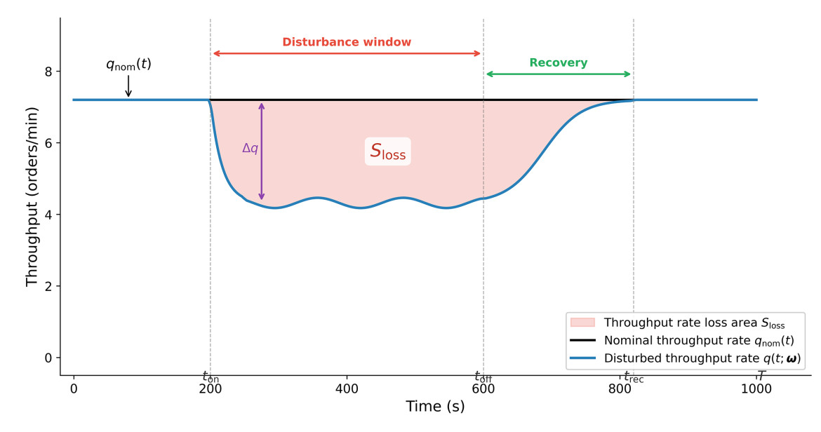
The system resilience is quantified using the resilience triangle approach[6,28]. Let $$ q_{\mathrm{nom}}(t) $$ denote the nominal (undisturbed) throughput rate curve and $$ q(t; \boldsymbol{\omega}) $$ the throughput rate curve under disturbance scenario $$ \boldsymbol{\omega} $$. The performance loss area during the observation window $$ [t_{\mathrm{on}}, T] $$ is

$$ S_{\mathrm{loss}} = \int_{t_{\mathrm{on}}}^{T} \max\!\bigl(q_{\mathrm{nom}}(t) - q(t; \boldsymbol{\omega}), \; 0\bigr)\, \mathrm{d}t, $$

which captures both the degradation phase ($$ t \in [t_{\mathrm{on}}, t_{\mathrm{off}}] $$) and any residual recovery lag ($$ t \in [t_{\mathrm{off}}, T] $$). The reference area under the nominal curve over the same interval is

$$ S_0 = \int_{t_{\mathrm{on}}}^{T} q_{\mathrm{nom}}(t)\, \mathrm{d}t.$$

The resilience index is then defined as

$$ R(\boldsymbol{\omega}) = 1 - \frac{S_{\mathrm{loss}}}{S_0}, $$

so that $$ R = 1 $$ corresponds to zero performance loss (perfect resilience) and smaller values indicate greater degradation. Compared with a simple endpoint ratio $$ Q(T)/Q_0 $$, this integral formulation accounts for the time-dependent degradation trajectory and recovery dynamics, consistent with the resilience triangle framework in the engineering resilience literature[6,28,29]. The concept is illustrated schematically in Figure 2.

Kriging-based resilience assessment of low-altitude logistics networks under multiple operational disturbances

Figure 2. Schematic illustration of the resilience triangle. The shaded area between the nominal throughput rate curve $$ q_{\mathrm{nom}}(t) $$ and the disturbed throughput rate curve $$ q(t;\boldsymbol{\omega}) $$ represents the loss area $$ S_{\mathrm{loss}} $$. The resilience index $$ R = 1 - S_{\mathrm{loss}}/S_0 $$ captures both the degradation depth and the recovery dynamics.

2.3 Multi-dimensional disturbance modelling

Operational disturbances are classified into three categories [Table 1], each parameterised by a scalar intensity that together form the disturbance vector $$ \boldsymbol{\omega} = (S, F, D)^{\!\top} $$. All disturbances are activated within a common temporal window $$ [t_{\mathrm{on}}, t_{\mathrm{off}}] = [200, 600] $$ s, but differ in spatial scope: the structural disturbance (NFZ) acts as a local square region centred at the airspace midpoint $$ (x_c, y_c) = (50, 50) $$; the functional disturbance (weather) applies globally across the entire $$ 100\; \times\; 100 $$ domain; and the informational disturbance (delay) affects all UTM decision processes system-wide.

Table 1

Summary of operational disturbance types and their modelled parameter ranges

TypePhysical mechanismDistributionRange
Structural ($$ S $$)No-fly zone blocks edgesUniform$$ [15, 55] $$
Functional ($$ F $$)Weather reduces flight speedUniform$$ [0.1, 0.8] $$
Informational ($$ D $$)Comm. delay slows decisionsUniform$$ [1, 40] $$

2.3.1 Structural disturbance (no-fly zone)

The NFZ is modelled as a square region of side length $$ S $$ (in grid units) centred at the airspace midpoint. The parameter $$ S $$ controls the spatial extent of the restricted area: a larger $$ S $$ blocks a greater number of air corridors, forcing UAVs onto longer detour paths or leaving them unable to reach their destinations. Let $$ \mathcal{Z}_{\mathrm{NFZ}}(S) = \{(x, y) : |x - 50| \leq S/2, \; |y - 50| \leq S/2\} $$ denote the square NFZ. During the disturbance window $$ [t_{\mathrm{on}}, t_{\mathrm{off}}] $$, any edge whose line segment geometrically intersects this region is removed from the available edge set:

$$ e \in E_{\mathrm{avail}}(t) \;\iff\; \neg\, \mathrm{intersects}\!\bigl(\overline{uv}, \, \mathcal{Z}_{\mathrm{NFZ}}(S)\bigr) \;\lor\; t \notin [t_{\mathrm{on}}, t_{\mathrm{off}}], $$

where $$ \overline{uv} $$ is the line segment connecting the two endpoints of edge $$ e = (u, v) $$, and $$ \mathrm{intersects}(\cdot, \cdot) $$ is a Boolean geometric intersection test. Edge removal is instantaneous: at $$ t = t_{\mathrm{on}} $$ all intersecting edges are simultaneously deactivated, and at $$ t = t_{\mathrm{off}} $$ they are restored. UAVs currently traversing a blocked edge enter the hold state at their last visited vertex and attempt re-planning (Section 2.1). The intensity parameter is sampled from $$ S \sim \mathrm{Uniform}(15, 55) $$. Here, $$ S = 15 $$ represents a localised restriction affecting only a few edges, while $$ S = 55 $$ covers over half the airspace diagonal.

2.3.2 Functional disturbance (weather degradation)

Adverse weather conditions (e.g., strong wind, heavy rain, reduced visibility) degrade the achievable flight speed of UAVs. Unlike the localised NFZ, the weather disturbance is modelled as a global effect covering the entire $$ 100\; \times\; 100 $$ domain (i.e., $$ \mathcal{R}_{\mathrm{weather}} = [0, L_x] \times [0, L_y] $$), representing large-scale meteorological phenomena. The degradation is parameterised by a weather disturbance intensity $$ F \in [0, 1) $$, where $$ F = 0 $$ denotes no weather impact and larger values represent more severe conditions. The resulting speed reduction factor applied to every edge in the network is

$$ \varphi_{\mathrm{weather}}(e, t) = \begin{cases} 1 - F, & \text{if } e \cap \mathcal{R}_{\mathrm{weather}} \neq \varnothing \text{ and } t \in [t_{\mathrm{on}}, t_{\mathrm{off}}], \\ 1, & \text{otherwise}, \end{cases} $$

where $$ e \cap \mathcal{R}_{\mathrm{weather}} \neq \varnothing $$ indicates that at least one endpoint of edge $$ e $$ falls inside the weather region. When $$ F = 0 $$, the speed factor equals 1 (nominal speed). As $$ F $$ increases, the effective speed $$ v_{\mathrm{eff}} $$ in Eq. (3) is proportionally reduced. For example, $$ F = 0.5 $$ yields a speed factor of $$ 1 - 0.5 = 0.5 $$, halving the flight speed and doubling the traversal time. The compounding effect is twofold: slower flights extend individual delivery times and delay UAV availability for subsequent orders. The intensity is sampled as $$ F \sim \mathrm{Uniform}(0.1, 0.8) $$. $$ F = 0.1 $$ represents mild degradation (10% speed loss) and $$ F = 0.8 $$ represents severe conditions (80% speed reduction).

2.3.3 Informational disturbance (communication delay)

Communication disruptions between the UAV fleet and the UTM system degrade the timeliness of two critical decision processes: dispatching (assigning idle UAVs to pending orders) and re-planning (computing alternative paths when edges are blocked). The delay is modelled as a multiplicative factor $$ D \geq 1 $$ that stretches both decision periods:

$$ \Delta t_{\mathrm{disp}}^{\prime} = D \cdot \Delta t_{\mathrm{disp}}, \qquad \Delta t_{\mathrm{replan}}^{\prime} = D \cdot \Delta t_{\mathrm{replan}}, $$

where $$ \Delta t_{\mathrm{disp}} $$ and $$ \Delta t_{\mathrm{replan}} $$ are the nominal dispatching and re-planning periods [Table 2]. When $$ D = 1 $$, the system operates at normal decision frequency. As $$ D $$ increases, the UTM system makes decisions less frequently, causing orders to wait longer in the pending queue and UAVs blocked by NFZs to remain in hold states for extended periods. For example, $$ D = 10 $$ means that the dispatching cycle increases from 1.0 to 10.0 s and the re-planning cycle from 2.0 to 20.0 s, effectively reducing the system's responsiveness by an order of magnitude. The parameter is sampled as $$ D \sim \mathrm{Uniform}(1, 40) $$, spanning from no delay to an extreme 40-fold slowdown in decision-making.

Table 2

Simulation parameters

ParameterSymbolValue
Grid size$$ L_x \times L_y $$100 × 100
Voronoi seed points$$ N_{\mathrm{seed}} $$140
Fleet size$$ N_{\mathrm{UAV}} $$80
Maximum speed$$ v_{\max} $$4.0 units/s
Route capacity$$ C_{\mathrm{route}} $$4 UAVs/edge
Simulation time step$$ \delta t $$0.5 s
Simulation horizon$$ T $$1,000 s
Order arrival rate$$ \lambda_{\mathrm{order}} $$6.0/s
Min. O–D distance$$ d_{\min} $$30 units
Dispatching period$$ \Delta t_{\mathrm{disp}} $$1.0 s
Re-planning period$$ \Delta t_{\mathrm{replan}} $$2.0 s
Disturbance window$$ [t_{\mathrm{on}}, t_{\mathrm{off}}] $$$$ [200, 600] $$ s

3. SIMULATION ENVIRONMENT AND SURROGATE MODEL CONSTRUCTION

3.1 Simulation platform and parameter settings

A discrete-event simulation platform is developed in Python to model the network described in Section 2.1. The simulation proceeds in fixed time steps of $$ \delta t = 0.5 $$ s over a horizon of $$ T = 1,000 $$ s. Each step executes: (1) order generation via a Poisson process; (2) edge occupancy counting; (3) greedy dispatching via A* with Euclidean heuristic; (4) re-planning for UAVs whose next edge is blocked; (5) UAV movement at the effective speed in Eq. (3); and (6) metrics recording.

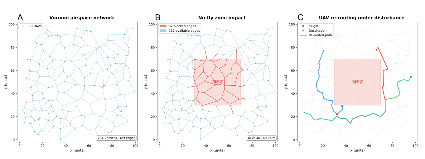
The Voronoi-based network is generated from $$ N_{\mathrm{seed}} = 140 $$ random seed points on a 100 × 100 grid, yielding a connected graph with approximately 230–245 vertices and 325–350 edges; the specific instance in Figure 3A contains 234 vertices and 329 edges. Key parameters are listed in Table 2.
Kriging-based resilience assessment of low-altitude logistics networks under multiple operational disturbances

Figure 3. Simulation environment. (A) Voronoi-based airspace network (234 vertices, 329 edges) with UAV initial positions; (B) example no-fly zone (shaded rectangle) blocking edges; (C) active UAV trajectories during a disturbance scenario showing re-routing behaviour.

Under nominal conditions (no disturbances active), the system completes approximately $$ Q_0 = 2,200 $$ orders by $$ t = T $$, as established from 15 independent baseline replications. The failure threshold is set to $$ Q_{\mathrm{th}} = 0.8\; \times\; 2,200 = 1,760 $$ orders.

Table 3 reports the operational metrics (defined in Section 2.2) under nominal conditions. The high UAV utilisation (97.2%) indicates near-full fleet capacity with minimal buffer against disturbances. The average delivery distance of 113.2 grid units corresponds to approximately 16% of the airspace diagonal. No orders were infeasible under the $$ d_{\min} = 30 $$ constraint, as the dense Voronoi graph (140 seeds) provides sufficient path diversity.

Table 3

Baseline network performance under nominal conditions (15 replications)

MetricMeanStdRange
Throughput rate $$ q $$ (orders/min)134.02.4[128.2, 137.6]
Avg. delivery distance $$ \bar{d} $$ (grid units)113.22.5[109.7, 119.3]
UAV utilisation $$ U $$ (%)97.20.07[97.1, 97.3]
Infeasible order fraction $$ \phi $$ (%)0.00.0

At the start of each replication, the $$ N_{\mathrm{UAV}} = 80 $$ UAVs are placed at vertices selected uniformly at random (with replacement) from $$ V $$, modelling a dispersed fleet with no predetermined depot structure. Each replication is assigned a deterministic random seed computed as $$ \mathit{seed} = 10,000\; +\; 100i\; +\; r $$, where $$ i $$ is the scenario index and $$ r $$ the replication index. This seed controls all stochastic elements—Voronoi seed point placement, order generation, and UAV initial positions—thereby ensuring full reproducibility. Because the global random state is re-seeded before each run, the network topology, demand sequence, and fleet deployment differ across replications, capturing the joint variability of network structure and operational randomness.

All simulation code is implemented in Python 3.10 using NumPy 1.24, SciPy 1.11, and scikit-learn 1.3.

3.2 Experimental design

Phase 1 — Single-disturbance experiments. Each disturbance type is first varied in isolation, as a one-factor-at-a-time screening, to characterise its marginal degradation curve and rank the three factors. Ten equally spaced intensity levels are used for each factor ($$ S \in \{10, 15.6, 21.1, \ldots, 60\} $$, $$ F \in \{0.1, 0.178, \ldots, 0.8\} $$, $$ D \in \{1, 5.1, \ldots, 37.5\} $$). To capture the full response of each factor from onset to saturation, the structural intensity is screened over the slightly wider interval $$ S \in [10, 60] $$, which brackets the range [15, 55] used later for the surrogate, while the weather ($$ F \in [0.1, 0.8] $$) spans its full modelled range and the delay ($$ D \in [1, 37.5] $$) covers a subset of its modelled range [1, 40] in Table 1. The complete delay range [1, 40] is later exercised in full by the conditional interaction analysis in Section 4.1. This screening confirms that the modelled ranges enclose the relevant transition region, on which the Phase-2 surrogate and all subsequent analyses are built. At each level, 15 independent replications are executed, yielding 3 × 10 × 15 = 450 simulation runs. The remaining two disturbance parameters are held at their nominal values ($$ S = 0 $$, $$ F = 0 $$, $$ D = 1 $$) so that each type's marginal effect is isolated. The degradation mode (linear, convex, or saturating), maximum performance loss, and critical threshold-crossing point are extracted to rank disturbance sensitivity and inform the dimension-reduction decision for Phase 2.

Phase 2 — Multi-disturbance training set. An LHS design with $$ n_{\mathrm{train}} = 80 $$ samples is generated in the two-dimensional disturbance space $$ (S, F) $$, where $$ S \sim \mathrm{Uniform}(15, 55) $$ and $$ F \sim \mathrm{Uniform}(0.1, 0.8) $$. The LHS procedure divides each marginal into $$ n_{\mathrm{train}} $$ equal-probability strata and draws one sample per stratum, then randomly pairs the marginal samples across dimensions. This guarantees uniform marginal coverage while avoiding the clustering that can occur with simple random sampling. The delay dimension $$ D $$ is excluded on the basis of the Phase-1 finding that its marginal sensitivity is substantially lower than the other two (see Section 4.1).

For each of the 80 training scenarios, $$ n_{\mathrm{rep}} = 5 $$ independent replications are executed. The mean completed-order count $$ \bar{Q} $$ is used as the response variable, giving a total of $$ 80 \times 5 = 400 $$ simulation runs. Averaging over replications reduces the noise level seen by the Kriging model and improves surrogate fit quality.

Phase 3 — Reliability and resilience analysis. After training, $$ N_{\mathrm{test}} = 10,000 $$ test scenarios are drawn from a uniform distribution over $$ (S, F) $$ and predicted instantaneously by the trained surrogate (each query returns a mean $$ \hat{\mu} $$ and standard deviation $$ \hat{\sigma} $$ in $$ \sim 0.1 $$ ms). Four analyses are then performed:

1. Failure probability field. For each of the 10,000 test points, $$ P_f $$ is computed via Eq. (21). The results are binned onto a $$ 50\; \times\; 50 $$ grid by nearest-neighbour assignment to produce a spatial risk map.

2. Resilience surface. An independent resilience surrogate (Kriging$$ _R $$, described in Section 3.3) is used to predict the resilience triangle index $$ R $$ in Eq. (13) directly on the same grid, and is rendered as a heatmap.

3. Sobol sensitivity indices. The first-order Sobol indices $$ S_S $$ and $$ S_F $$ are estimated by a variance-decomposition approach[30]: the total output variance $$ \sigma_Y^2 $$ of the 10,000 predictions is computed, then each input is fixed at a sequence of values while the other is marginalised, yielding the conditional variance contributions.

4. Critical failure boundary. All test points satisfying $$ |\hat{Q} - Q_{\mathrm{th}}| < 0.05\, Q_{\mathrm{th}} $$ (i.e. within a 5% band of the threshold) are extracted and plotted in the $$ (S, F) $$ space to delineate the transition zone between safe and failure regions.

3.3 Kriging surrogate model: formulation, training, and computational efficiency

Model formulation. A Kriging model (Gaussian process regression) maps the disturbance vector $$ \boldsymbol{\omega} = (S, F)^{\!\top} $$ to the performance metric $$ Q(T; \boldsymbol{\omega}) $$. The predictor is

$$ \hat{Q}(\boldsymbol{\omega}) = \sum\limits_{i=1}^{n} \alpha_i \, k(\boldsymbol{\omega}, \boldsymbol{\omega}_i), $$

where $$ \{(\boldsymbol{\omega}_i, Q_i)\}_{i=1}^{n} $$ are training observations, $$ \alpha_i $$ are optimised weights, and $$ k(\cdot, \cdot) $$ is a radial basis function (RBF) kernel with automatic relevance determination (ARD):

$$ k(\boldsymbol{\omega}, \boldsymbol{\omega}') = \sigma_f^2 \exp\!\left( -\sum\limits_{j=1}^{d} \frac{(\omega_j - \omega_j')^2}{2\, \ell_j^2} \right), $$

where $$ \sigma_f^2 $$ is the signal variance and $$ \ell_j $$ is the characteristic length scale along the $$ j $$-th axis. The ARD structure assigns an independent length scale to each input dimension: a short $$ \ell_j $$ indicates that the output is highly sensitive to the $$ j $$-th input, while a long $$ \ell_j $$ implies weak dependence.

Hyperparameter optimisation. The optimisable hyperparameter vector is $$ \boldsymbol{\theta} = (\sigma_f, \, \ell_1, \ldots, \ell_d) $$, comprising the signal amplitude and per-dimension length scales. These are determined by maximising the log marginal likelihood of the training data:

$$ \log p(\mathbf{y} \mid \mathbf{X}, \boldsymbol{\theta}) = -\tfrac{1}{2}\, \mathbf{y}^{\!\top} \mathbf{K}_y^{-1}\, \mathbf{y} -\tfrac{1}{2}\, \log|\mathbf{K}_y| -\tfrac{n}{2}\, \log 2\pi, $$

where $$ \mathbf{y} = (Q_1, \ldots, Q_n)^{\!\top} $$ is the vector of training responses, $$ \mathbf{X} = (\boldsymbol{\omega}_1, \ldots, \boldsymbol{\omega}_n) $$ is the training input matrix, and $$ \mathbf{K}_y = \mathbf{K} + \alpha\, \mathbf{I} $$ is the regularised covariance matrix with entries $$ K_{ij} = k(\boldsymbol{\omega}_i, \boldsymbol{\omega}_j) $$. The diagonal nugget $$ \alpha = 10^{-6} $$ is a fixed regularisation constant that ensures numerical stability of the Cholesky decomposition. Because each training response $$ \bar{Q}_i $$ is already the mean of 5 replications, the residual observation noise is small and does not require a separate noise kernel.

The first term in Eq. (19) penalises data misfit, the second penalises model complexity, and the third is a normalisation constant. Optimisation is performed using L-BFGS-B with $$ n_{\mathrm{restart}} = 10 $$ random restarts to mitigate local optima. The training targets are standardised ($$ y \leftarrow (y - \bar{y})/s_y $$) before fitting to improve numerical conditioning. Predictions are back-transformed to the original scale.

Training results. The model is trained on $$ n = 80 $$ LHS design points. After optimisation, the maximised log marginal likelihood is $$ \log p(\mathbf{y} \mid \mathbf{X}, \hat{\boldsymbol{\theta}}) = -38.92 $$, and the optimised kernel is $$ k = 0.773^2 \times \mathrm{RBF}(\ell_S = 2.176, \; \ell_F = 0.132) $$. The length-scale ratio $$ \ell_S / \ell_F \approx 16.5 $$ confirms that the performance surface varies much more rapidly along the weather axis ($$ F $$), requiring only $$ \ell_F = 0.132 $$ units to capture its steep gradient, whereas a comparatively gentle $$ \ell_S = 2.176 $$ suffices for the structural axis ($$ S $$). The training data spans a response range of $$ [1,403.6, \, 1,980.8] $$ completed orders with mean $$ \bar{y} = 1633.2 $$ and standard deviation $$ s_y = 153.4 $$.

Computational efficiency. A direct Monte Carlo evaluation of the failure probability field at a resolution of $$ 50 \times 50 = 2{, }500 $$ grid points with 5 replications per point would require 12,500 simulation runs ($$ {\approx}86 $$ h). The Kriging approach requires only 400 training runs ($$ {\approx}3.4 $$ h), after which the 2,500-point prediction takes less than one second—a speed-up of approximately 25-fold.

Resilience surrogate (Kriging$$ _R $$). The performance surrogate described above (hereafter Kriging$$ _Q $$) predicts $$ Q(T) $$ and is used for failure probability estimation, Sobol sensitivity analysis, and critical failure boundary identification. To capture the degradation and recovery dynamics reflected in the resilience index $$ R $$ in Eq. (13), we train a second surrogate—Kriging$$ _R $$—using training labels derived from the full throughput rate trajectory $$ q(t) $$.

For each of the 80 LHS training scenarios, the full time-series outputs (throughput buckets, completed orders, and backlog over the 1,000 s horizon) were saved during Phase 2 simulation runs. From these trajectories, the resilience triangle index $$ R $$ is computed via Eqs. (11)–(13) using the disturbance window $$ [200, 600] $$ s and the nominal throughput rate $$ q_{\mathrm{nom}}(t) $$ estimated from the pre-disturbance period. The mean $$ R $$ over 5 replications serves as the training label, yielding 80 $$ (S, F, \bar{R}) $$ training triplets without additional simulation cost.

A Gaussian process with an RBF–ARD kernel (identical in form to Eq. (18)) is fitted to these data. The optimised kernel is

$$ k_R(\boldsymbol{\omega}, \boldsymbol{\omega}') = 0.731^2 \times \mathrm{RBF}\!\left(\ell_S = 5.65, \; \ell_F = 0.051\right). $$

Key training statistics: $$ R $$ range $$ [0.540, 0.874] $$, mean $$ = 0.668 $$, std $$ = 0.090 $$. The length-scale ratio $$ \ell_S / \ell_F \approx 111 $$ indicates that weather intensity $$ F $$ drives far more rapid resilience degradation than structural disturbance $$ S $$, consistent with the Sobol analysis from Kriging$$ _Q $$. The much shorter $$ \ell_F $$ in Kriging$$ _R $$ (0.051 vs. 0.132 in Kriging$$ _Q $$) reflects the additional sensitivity introduced by the integral formulation. Because $$ R $$ accumulates performance loss over the entire disturbance window, sustained speed reduction has a magnified effect compared with the endpoint metric $$ Q(T) $$.

3.4 Model validation and uncertainty quantification

For each test point $$ \boldsymbol{\omega}^{*} $$, the Kriging model returns a mean prediction $$ \hat{\mu}(\boldsymbol{\omega}^{*}) $$ and a predictive standard deviation $$ \hat{\sigma}(\boldsymbol{\omega}^{*}) $$. This built-in uncertainty quantification is a well-established advantage of Gaussian process models over deterministic surrogates[26,31].

The failure probability at a given parameter combination is computed by integrating over the predictive distribution:

$$ P_f(\boldsymbol{\omega}^{*}) = \Phi\!\left( \frac{Q_{\mathrm{th}} - \hat{\mu}(\boldsymbol{\omega}^{*})}{\hat{\sigma}(\boldsymbol{\omega}^{*})} \right), $$

where $$ \Phi(\cdot) $$ is the standard normal CDF. This formulation, known as the U-learning function in active-learning reliability analysis[25,27], naturally accounts for both the predicted mean and the prediction uncertainty, providing a more conservative risk estimate than a deterministic threshold comparison.

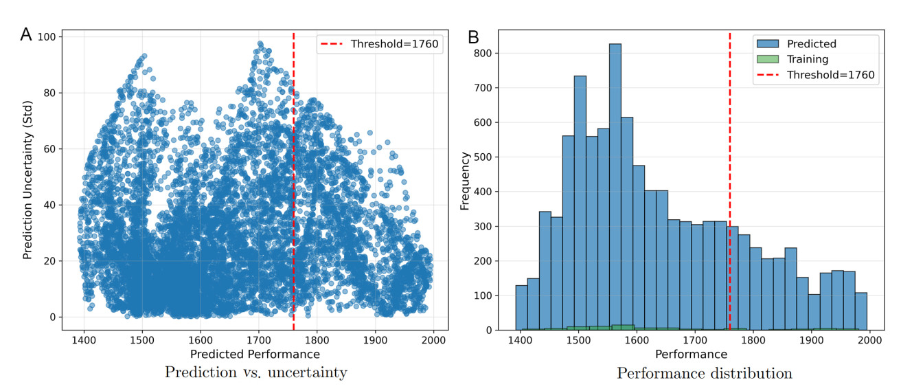
To assess model credibility, we examine the predictive standard deviation across all 10,000 test points. Figure 4 plots each test point's predicted performance ($$ \hat{\mu} $$) against its prediction standard deviation ($$ \hat{\sigma} $$), with the failure threshold $$ Q_{\mathrm{th}} = 1,760 $$ shown as a vertical dashed line. The results show that the predicted performance spans [1,392.5, 1,995.1] completed orders with a global mean of 1,638.6. The prediction confidence is classified into three tiers:

Kriging-based resilience assessment of low-altitude logistics networks under multiple operational disturbances

Figure 4. Kriging model uncertainty analysis based on 10,000 test scenarios. (A) Predicted performance $$ \hat{\mu} $$ vs. predictive standard deviation $$ \hat{\sigma} $$. (B) Performance distribution of test predictions (blue) and 80 training samples (green). The red dashed line marks the failure threshold $$ Q_{\mathrm{th}} = 1,760 $$.

● High confidence ($$ \hat{\sigma} < 40 $$): approximately 85% of predictions, located near training samples.

● Moderate confidence ($$ 40 \leq \hat{\sigma} < 60 $$): approximately 13%, in sparser regions of the design.

● Low confidence ($$ \hat{\sigma} \geq 60 $$): approximately 2%, in extreme extrapolation regions.

With 85% of predictions falling in the high-confidence tier and 98% in the high-or-moderate tier, the 80-point LHS design provides reasonable coverage of the $$ (S, F) $$ parameter space for mapping global risk trends. However, the remaining 2% of low-confidence points—concentrated near parameter extremes—warrant caution when interpreting predictions in those regions. Targeted infill sampling (e.g., via active learning) could improve local accuracy if higher fidelity is required.

The model is further validated through a multi-threshold reliability analysis [Table 4]. For each threshold level $$ Q_{\mathrm{th}} $$, two independent failure probability estimates are computed: (ⅰ) a probabilistic estimate obtained by averaging $$ P_f(\boldsymbol{\omega}^{*}) $$ from Eq. (21) over all 10,000 test points, and (ⅱ) a deterministic estimate computed as the fraction of test points whose mean prediction $$ \hat{\mu} $$ falls below $$ Q_{\mathrm{th}} $$. The two estimates agree to within 0.5% across all threshold levels, confirming the internal consistency of the Kriging predictions and indicating that predictive uncertainty does not materially bias the failure probability estimates.

Table 4

Multi-threshold reliability analysis results

Threshold level$$ Q_{\mathrm{th}} $$$$ P_f $$ (probabilistic)$$ P_f $$ (deterministic)
90% of $$ Q_0 $$19800.9890.993
80% of $$ Q_0 $$17600.7770.782
70% of $$ Q_0 $$15400.2880.286
50% of $$ Q_0 $$1100$$ {\approx}0 $$0.000

4. RESULTS AND DISCUSSION

4.1 Single-disturbance degradation analysis

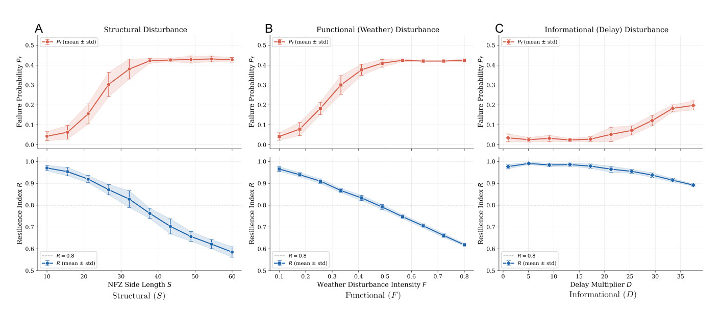
Each disturbance type is applied in isolation, while the remaining two are held at nominal values. For every disturbance, 10 intensity levels are evaluated with 15 replications per level, yielding 150 simulation runs per type. The results are summarised in Figure 5.
Kriging-based resilience assessment of low-altitude logistics networks under multiple operational disturbances

Figure 5. Single-disturbance degradation analysis. Each subfigure contains two vertically stacked panels: the upper panel shows the failure probability $$ P_f $$ and the lower panel shows the resilience index $$ R $$ (both reported as mean $$ \pm $$ standard deviation across 15 replications). The grey dashed line in the lower panel marks $$ R = 0.8 $$ as a reference. (A) Structural disturbance ($$ S \in [10, 60] $$): $$ P_f $$ rises sharply between $$ S = 20 $$ and $$ S = 35 $$ before saturating near 0.43; $$ R $$ decreases near-linearly from 0.97 to 0.59. (B) Functional disturbance ($$ F \in [0.1, 0.8] $$): $$ P_f $$ exhibits an S-shaped increase; $$ R $$ crosses the 0.8 reference near $$ F \approx 0.5 $$. (C) Informational disturbance ($$ D \in [1, 37.5] $$): $$ P_f $$ remains below 0.20 and $$ R $$ stays above 0.89 throughout, confirming its limited impact.

Structural disturbance. The structural disturbance exhibits a predominantly linear degradation pattern. The resilience index decreases steadily from $$ R = 0.970 $$ at $$ S = 10 $$ to $$ R = 0.585 $$ at $$ S = 60 $$, a total resilience loss of approximately 38.5%. Failure probability rises sharply between $$ S = 21 $$ and $$ S = 27 $$ (from $$ P_f = 0.15 $$ to $$ P_f = 0.30 $$), then saturates near $$ P_f \approx 0.43 $$ for $$ S > 38 $$. The linear behaviour can be attributed to the Voronoi network's multiple alternative routes; as the NFZ grows, more edges are blocked, and detour lengths increase proportionally.

Functional disturbance. In contrast, the functional disturbance produces a markedly nonlinear, convex degradation curve. As $$ F $$ increases from 0.1 (mild weather) towards 0.8 (severe weather), performance degrades in three distinct phases:

● A mild-impact zone ($$ F < 0.3 $$): the resilience remains above $$ R = 0.91 $$, and the fleet absorbs the speed reduction with minimal throughput loss.

● A transition zone ($$ F \approx 0.4 $$): the resilience drops from $$ R = 0.87 $$ to $$ R = 0.79 $$, and failure probability rises sharply from $$ P_f = 0.30 $$ to $$ P_f = 0.41 $$.

● A severe-impact zone ($$ F > 0.6 $$): the degradation curve steepens. At $$ F = 0.8 $$, the resilience index falls to $$ R = 0.618 $$ (a 38.2% loss).

This nonlinearity arises because flight speed reductions simultaneously increase delivery time per order and delay UAV re-availability, creating a compounding throughput loss. Among the three disturbance types, weather degradation produces the steepest gradient in resilience loss per unit change in its parameter.

Informational disturbance. The informational disturbance exhibits a mildly nonlinear pattern with relatively low sensitivity. The resilience index remains above $$ R = 0.95 $$ for $$ D < 25 $$. Beyond $$ D = 30 $$, degradation accelerates slightly, but the maximum resilience loss at $$ D = 37.5 $$ is only 10.8% ($$ R = 0.892 $$). The fleet of 80 UAVs provides sufficient capacity to absorb moderate decision latency.

Comparative summary. As summarised in Table 5, these findings motivate two modelling decisions for Phase 2: (1) the delay parameter $$ D $$ is excluded from the Kriging surrogate to reduce input dimensionality from three to two, improving surrogate accuracy with the same training budget, and (2) the remaining two parameters $$ (S, F) $$ warrant joint multi-disturbance analysis.

Table 5

Comparative summary of single-disturbance degradation analysis

TypeDegradation modeSensitivityCritical pointMax. loss
Structural ($$ S $$)LinearModerate$$ S \approx 27 $$$$ \sim 38\% $$
Functional ($$ F $$)Nonlinear (convex)Highest$$ F \approx 0.4 $$$$ \sim 38\% $$
Informational ($$ D $$)Mildly nonlinearLowest$$ D \approx 30 $$$$ \sim 11\% $$

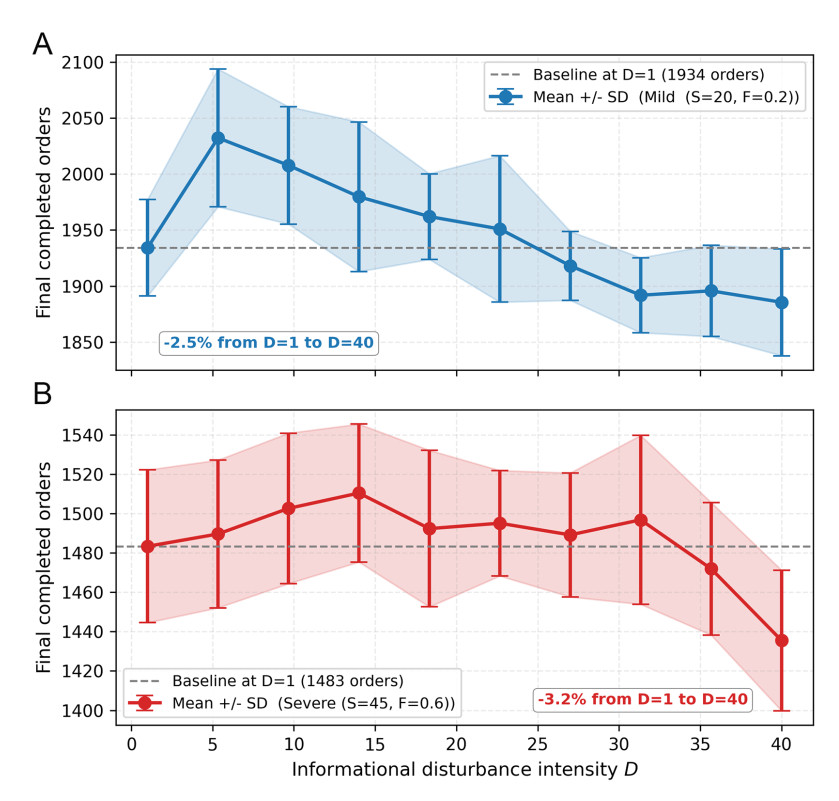
Conditional interaction analysis for the informational disturbance. To verify that the low marginal sensitivity of $$ D $$ observed in Phase 1 (where $$ S = 0 $$ and $$ F = 0 $$) is not an artefact of the benign background conditions, we conduct a conditional interaction analysis. Two background scenarios are fixed—mild ($$ S = 20 $$, $$ F = 0.2 $$) and severe ($$ S = 45 $$, $$ F = 0.6 $$)—while $$ D $$ is swept from 1 to 40 across 10 levels with 15 replications each (300 additional runs). The results [Figure 6] show limited marginal throughput degradation under both conditions: $$ -2.5\% $$ under the mild background and $$ -3.2\% $$ under the severe background. The magnitude of $$ D $$'s effect does not increase when $$ S $$ and $$ F $$ are large, indicating an additive rather than synergistic interaction. Under severe structural–weather disturbances, throughput is already constrained by physical factors (blocked routes, reduced speed), so slower decision-making has a bounded marginal impact.
Kriging-based resilience assessment of low-altitude logistics networks under multiple operational disturbances

Figure 6. Conditional interaction analysis: throughput degradation as a function of communication delay $$ D $$ under (A) mild ($$ S = 20 $$, $$ F = 0.2 $$) and (B) severe ($$ S = 45 $$, $$ F = 0.6 $$) backgrounds. Error bars indicate mean ± standard deviation across 15 replications.

These results confirm that the cross-interaction effect of $$ D $$ with the other two parameters is small. They further justify concentrating the surrogate modelling effort on the structural–functional disturbance combination $$ (S, F) $$, whose joint impact on performance and resilience is substantially larger.

4.2 Multi-disturbance analysis

The trained Kriging surrogates are used to explore the two-dimensional disturbance space $$ (S, F) $$ comprehensively. The performance surrogate Kriging$$ _Q $$ (predicting endpoint cumulative orders $$ Q(T) $$) supports global sensitivity analysis via Sobol indices (Section 4.2.1), failure probability field mapping (Section 4.2.2), and critical failure boundary identification (Section 4.2.3). The resilience surrogate Kriging$$ _R $$ (predicting the integral resilience triangle index $$ R $$) is used to construct the resilience surface characterisation (Section 4.2.4).

4.2.1 Global sensitivity analysis via Sobol indices

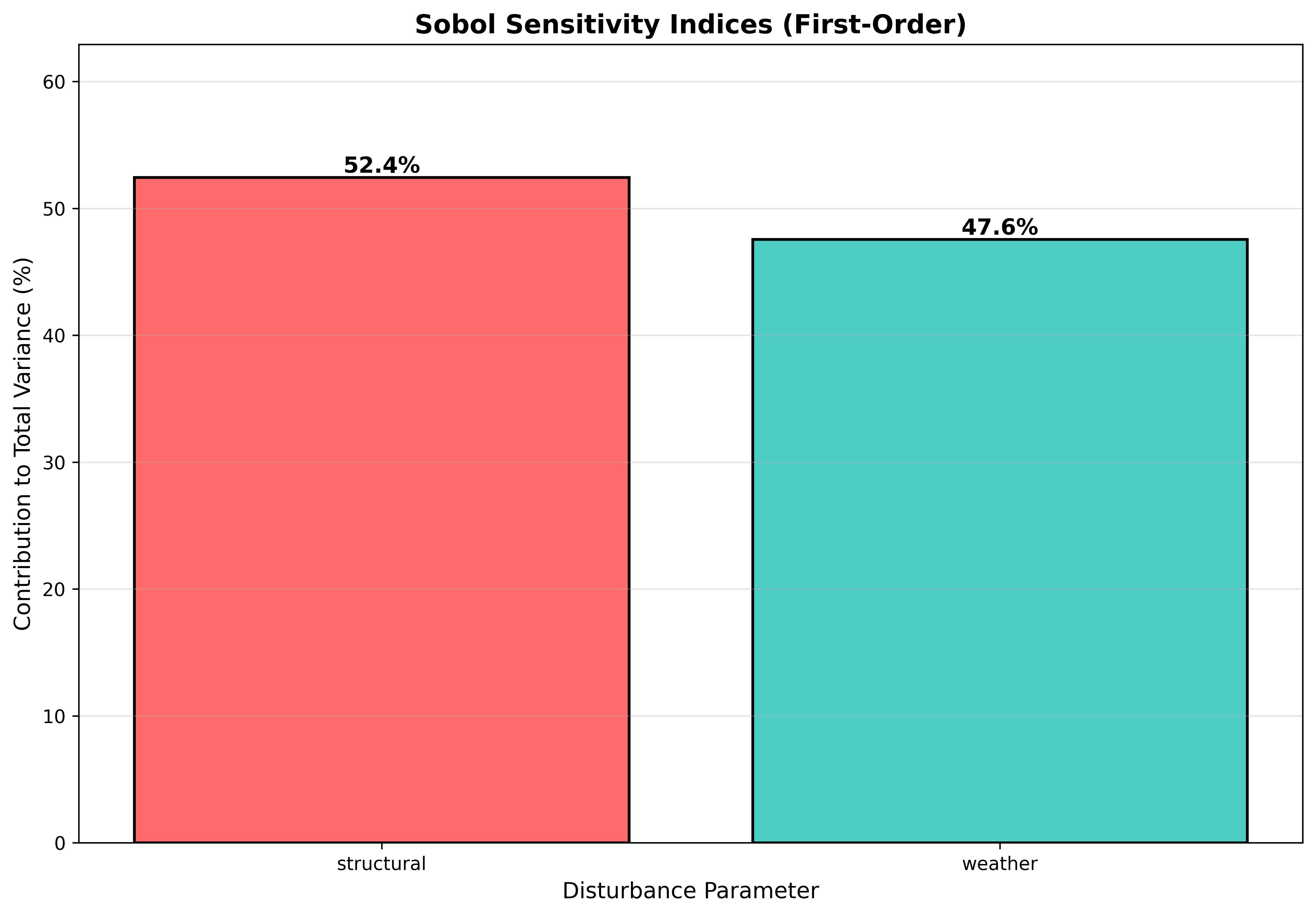
A variance-based Sobol sensitivity analysis is conducted using 10,000 uniformly sampled scenarios predicted by the Kriging model. The total output variance is $$ \sigma^2_Y = 21{, }206.2 $$. The first-order Sobol indices are:

● Structural parameter $$ S $$: $$ S_S = 0.524 $$ (52.4% of total variance).

● Weather parameter $$ F $$: $$ S_F = 0.476 $$ (47.6% of total variance).

The near-parity between the two indices is shown in Figure 7. Although the single-disturbance analysis identified weather as the most sensitive factor per unit change, the structural parameter's broader range ($$ [15, 55] $$ vs. $$ [0.1, 0.8] $$) compensates for its lower per-unit sensitivity, making it slightly more influential in the joint space. Neither parameter can be neglected without underestimating systemic risk.

Kriging-based resilience assessment of low-altitude logistics networks under multiple operational disturbances

Figure 7. First-order Sobol sensitivity indices. The structural parameter $$ S $$ contributes 52.4% and the weather parameter $$ F $$ contributes 47.6% to the total output variance ($$ \sigma^2_Y = 21{, }206.2 $$).

4.2.2 Failure probability field mapping

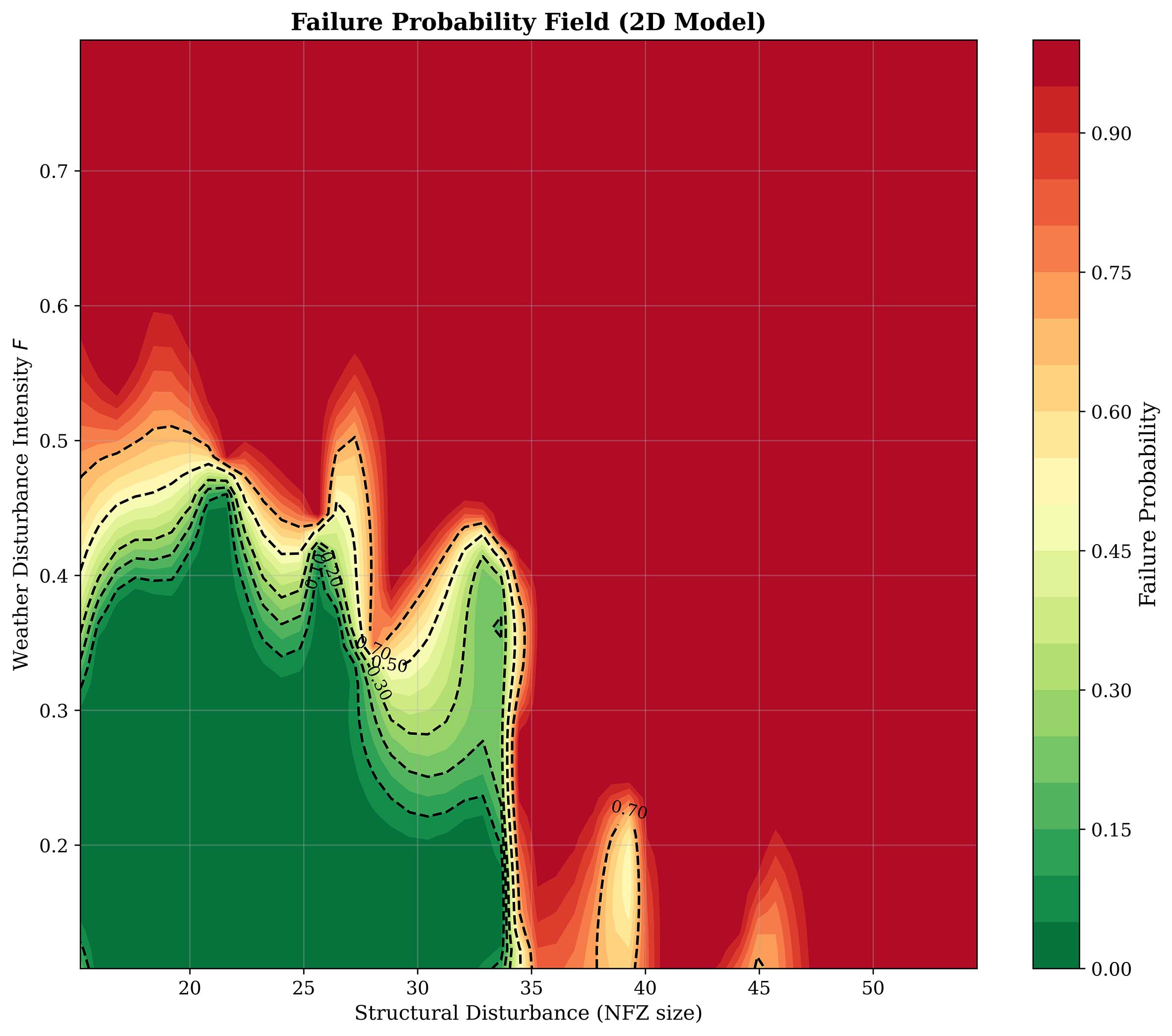
Using Eq. (21), the failure probability $$ P_f $$ is computed on a $$ 50\; \times\; 50 $$ grid. The field shows a monotonic risk gradient from the lower-left corner (low $$ S $$, low $$ F $$: mild conditions) to the upper-right corner (high $$ S $$, high $$ F $$: severe conditions). Three risk zones are identified:

● Very high risk zone ($$ P_f > 0.9 $$): covers $$ \sim 72\% $$ of the parameter space, where ($$ S > 35 $$) or ($$ F > 0.5 $$).

● Transition zone ($$ 0.1 < P_f \leq 0.9 $$): covers only $$ \sim 13.4\% $$, the narrow transition band between the safe zone and the very-high-risk zone.

● Safe zone ($$ P_f \leq 0.1 $$): covers $$ \sim 14.6\% $$, where $$ S < 35 $$ and $$ F < 0.3 $$.

The safe zone covers only about 14.6% of the parameter space [Figure 8], indicating high vulnerability to combined disturbances across a wide range of operating conditions.
Kriging-based resilience assessment of low-altitude logistics networks under multiple operational disturbances

Figure 8. Failure probability field $$ P_f(S, F) $$ over the two-dimensional disturbance parameter space. The colour scale ranges from deep green ($$ P_f \leq 0.1 $$, safe) to deep red ($$ P_f > 0.9 $$, very high risk). The x-axis represents the structural disturbance intensity S and the y-axis represents the weather disturbance intensity F (higher F = more severe weather). The black dashed lines are iso-probability contours at $$ P_f $$ = 0.1, 0.2, 0.3, 0.5, and 0.7.

Among the 10,000 sampled test scenarios, the lowest predicted performance occurs at $$ (S = 52.5, F = 0.696) $$ with $$ \hat{Q} = 1,392.5 \pm 28.9 $$ orders (36.7% degradation). The highest performance is found at $$ (S = 17.4, F = 0.183) $$ with $$ \hat{Q} = 1,995.1 \pm 18.0 $$ orders (9.3% degradation).

The theoretical worst case corresponds to the parameter-space boundary $$ (S = 55, F = 0.8) $$, where the maximum structural disruption is combined with the most severe weather. The observed worst-case sample $$ (52.5, 0.696) $$ lies close to this boundary, and the failure probability field [Figure 8] confirms that $$ P_f $$ approaches 1.0 in this extreme region. The prediction uncertainty in the worst-case region ($$ \hat{\sigma} \approx 28.9 $$) is moderately higher than in the best-case region ($$ \hat{\sigma} \approx 18.0 $$), reflecting both greater output variability under severely degraded conditions and sparser training-sample coverage near parameter extremes.

4.2.3 Critical failure boundary identification

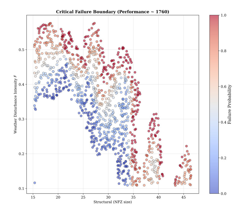
The critical failure boundary is the locus of parameter combinations satisfying $$ |\hat{Q} - Q_{\mathrm{th}}| < 0.05 \cdot Q_{\mathrm{th}} $$ (i.e, . $$ 1,672 < \hat{Q} < 1,848 $$). The boundary consists of approximately 1,348 parameter combinations and traces a diagonal band from the lower-left (safe region: low $$ S $$, low $$ F $$) to the upper-right (failure region: high $$ S $$, high $$ F $$), as shown in Figure 9.
Kriging-based resilience assessment of low-altitude logistics networks under multiple operational disturbances

Figure 9. Critical failure boundary in the $$ (S, F) $$ parameter space. Each dot represents a disturbance scenario whose predicted performance lies within 5% of the failure threshold ($$ 1,672 < \hat{Q} < 1,848 $$); colour indicates the local failure probability (blue = safe, red = dangerous). The diagonal boundary band separates the safe region (lower-left: low $$ S $$, low $$ F $$) from the failure region (upper-right: high $$ S $$, high $$ F $$) and spans approximately 27% of the parameter space, reflecting prediction uncertainty.

Three operationally relevant insights emerge:

1. Asymmetric recovery effectiveness. Reducing weather severity (decreasing $$ F $$) yields a larger safety margin than reducing structural disruption (decreasing $$ S $$). Investing in weather-adaptive UAV capabilities may be more cost-effective than strategies focused solely on NFZ avoidance.

2. Early warning. The boundary band thickness ($$ \sim 27\% $$ of the parameter space) provides a natural basis for an early-warning system: preliminary alert near the outer edge, elevated warning in the interior, and emergency activation upon crossing to the dangerous side.

3. Real-time safety distance. The current disturbance state $$ (S_{\mathrm{now}}, F_{\mathrm{now}}) $$ can be compared against the boundary to compute a continuously updated safety distance metric for traffic managers.

4.2.4 Resilience surface characterisation

The preceding three analyses (Sobol indices, failure probability field, and critical boundary) are all based on the performance surrogate Kriging$$ _Q $$. The resilience surface is instead constructed using the dedicated resilience surrogate Kriging$$ _R $$ (Section 3.3), which directly predicts the resilience triangle index $$ R(\boldsymbol{\omega}) $$ in Eq. (13), computed from the complete throughput rate trajectory $$ q(t) $$.

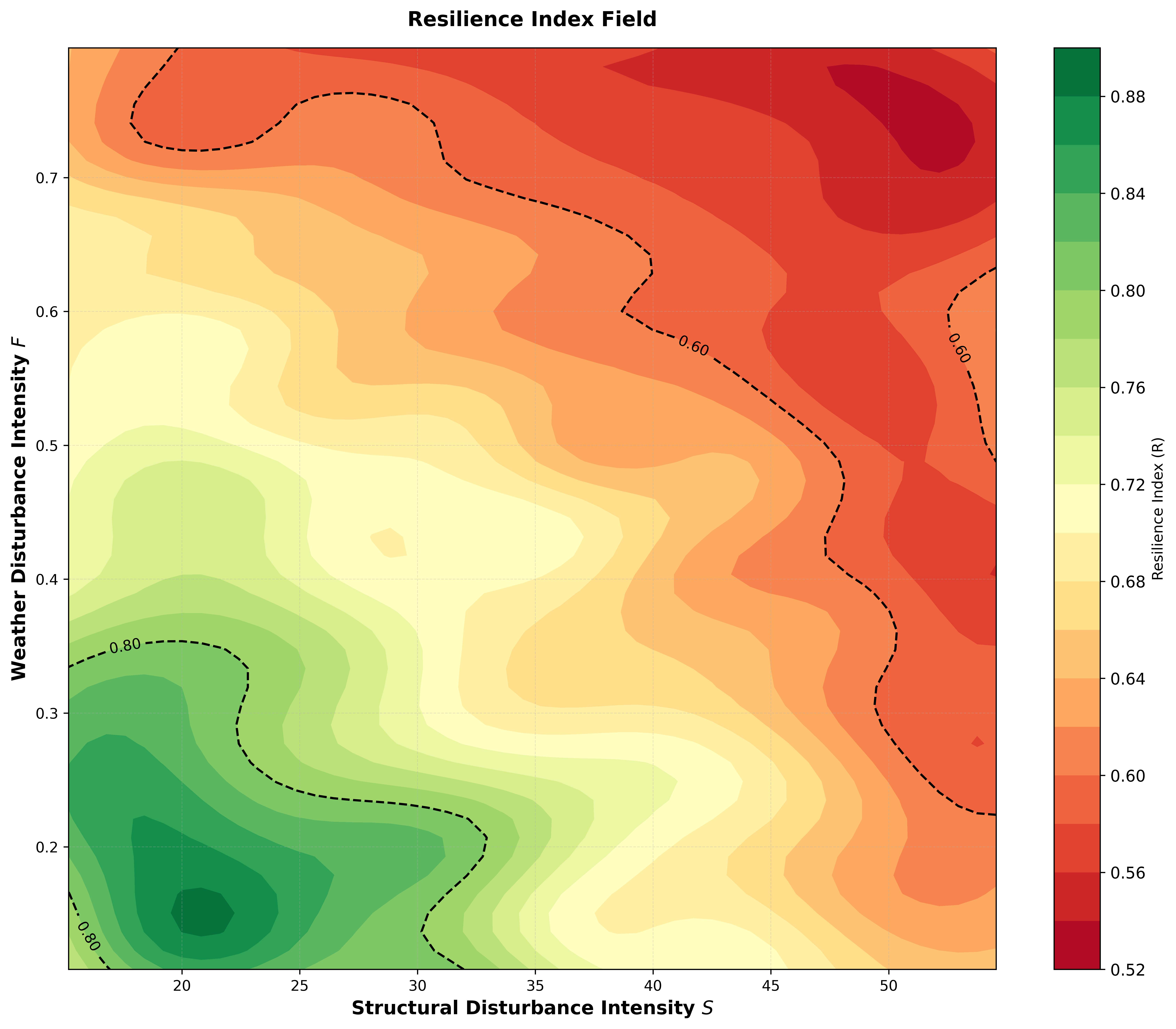
The Kriging$$ _R $$ predictions are evaluated on a $$ 50\; \times\; 50 $$ grid over the $$ (S, F) $$ parameter space. The disturbance space is partitioned into three resilience zones [Figure 10]:

Kriging-based resilience assessment of low-altitude logistics networks under multiple operational disturbances

Figure 10. Resilience surface predicted by Kriging$$ _R $$ over the $$ (S, F) $$ disturbance parameter space. The colour scale represents the resilience triangle index $$ R $$ in Eq. (13). Three zones are delineated: high-resilience ($$ R \geq 0.8 $$, 10.9%), medium-resilience ($$ 0.6 \leq R < 0.8 $$, 62.8%), and low-resilience ($$ R < 0.6 $$, 26.4%). The contour lines mark $$ R = 0.8 $$ and $$ R = 0.6 $$.

● High-resilience zone ($$ R \geq 0.8 $$): concentrated in the low-$$ S $$, low-$$ F $$ corner, occupying 10.9% of the parameter space. In this region, the network absorbs disturbances with limited performance degradation.

● Medium-resilience zone ($$ 0.6 \leq R < 0.8 $$): covering the broad transitional region, accounting for 62.8%. Performance is noticeably degraded, but the system maintains partial functionality.

● Low-resilience zone ($$ R < 0.6 $$): located in the high-$$ S $$, high-$$ F $$ region where structural and weather disturbances superimpose, covering 26.4%. The network suffers severe throughput loss with slow or incomplete recovery.

The $$ R = 0.8 $$ and $$ R = 0.6 $$ contour lines delineate the boundaries between these zones. The surface is strongly anisotropic: the gradient along $$ F $$ is substantially steeper than along $$ S $$, consistent with the Kriging$$ _R $$ length-scale ratio $$ \ell_S / \ell_F \approx 111 $$ in Eq. (20). The diagonal alignment of the medium-resilience zone indicates that the two disturbance types interact approximately additively.

Together with the failure probability field and critical boundary, the resilience surface [Figure 10] completes a comprehensive risk landscape that can inform both strategic planning (fleet sizing, network design) and tactical decision-making (dynamic dispatching, re-routing protocols).

5. CONCLUSIONS

This paper has proposed a Kriging-based resilience assessment framework for low-altitude UAV logistics networks subject to multiple operational disturbances. A discrete-event simulation environment was developed, integrating Voronoi-based airspace topology, A* path planning, and dynamic dispatching with re-planning. Three disturbance types—structural (no-fly zones), functional (weather degradation), and informational (communication delay)—were modelled and evaluated both individually and jointly. The principal findings are as follows:

1. Weather degradation is the most sensitive individual factor per unit change (critical transition at $$ F \approx 0.4 $$, maximum resilience loss $$ \sim 38\% $$), closely followed by structural disruption (linear degradation, $$ \sim 38\% $$ loss). Informational delay has a limited impact ($$ \sim 11\% $$ loss).

2. A Kriging surrogate trained on 80 LHS samples achieves a 25-fold speed-up over direct Monte Carlo simulation, with 85% of predictions in the high-confidence region ($$ \hat{\sigma} < 40 $$).

3. Sobol global sensitivity analysis shows that the structural and weather parameters contribute 52.4% and 47.6% to total performance variance, respectively, indicating comparable influence on network degradation.

4. Only $$ \sim 14.6\% $$ of the parameter space qualifies as a safe operating zone ($$ P_f \leq 0.1 $$), and the critical failure boundary traces a diagonal band that provides a quantitative basis for early-warning systems and real-time safety distance calculations.

5. The resilience surface constructed from the dedicated Kriging$$ _R $$ surrogate partitions the disturbance space into three zones: high-resilience ($$ R \geq 0.8 $$, 10.9%), medium-resilience ($$ 0.6 \leq R < 0.8 $$, 62.8%), and low-resilience ($$ R < 0.6 $$, 26.4%). The medium- and low-resilience zones together account for 89.1% of the parameter space, indicating that the network is vulnerable over a wide range of combined disturbances.

Several limitations suggest directions for future work. The disturbance model assumes spatially uniform, step-switched profiles, and future work could introduce stochastic spatio-temporal fields (e.g., Gaussian weather models, Karhunen–Loève representations) for greater realism. The resilience assessment also relies on a deterministic disturbance window and would benefit from stochastic durations and recovery profiles. Moreover, the greedy dispatching policy should be benchmarked against anticipatory and DRL-based schedulers[19,21,22,24] within the same disturbance space. Finally, validation with real UAV delivery trial data is needed to calibrate the simulation and disturbance distributions for specific deployment contexts.

DECLARATIONS

Authors' contributions

Methodology, writing - original draft, investigation, conceptualisation: Yao, A.

Investigation, visualisation: Song, X.; Li, S.; Feng, K.

Writing - reviewing, supervision: Li, H.; Zhou, H.

Availability of data and materials

The authors generated all data and materials used in the research as an integral part of the study, with explicit details provided in the methodology section of the manuscript. These are available from the corresponding author upon reasonable request.

AI and AI-assisted tools statement

Not applicable.

Financial support and sponsorship

This work was supported by the National Key Research and Development Program of China (2023YFB4302901) and the Civil Aviation Safety Capacity Building Project of the Civil Aviation Administration of China (HA202511).

Conflicts of interest

All authors declared that there are no conflicts of interest.

Ethical approval and consent to participate

Not applicable.

Consent for publication

Not applicable.

Copyright

© The Author(s) 2026.

REFERENCES

1. Sengupta, R.; Bulusu, V.; Mballo, C. E.; Onat, E. B.; Cao, S. Urban air mobility research: challenges and opportunities. Annu. Rev. Control. Robot. Auton. Syst. 2025, 8, 407-31.

2. Shavarani, S. M.; Nejad, M. G.; Rismanchian, F.; Izbirak, G. Application of hierarchical facility location problem for optimization of a drone delivery system: a case study of Amazon Prime Air in the city of San Francisco. Int. J. Adv. Manuf. Technol. 2017, 95, 3141-53.

3. Kim, J.; Atkins, E. Airspace geofencing and flight planning for low-altitude, urban, small unmanned aircraft systems. Appl. Sci. 2022, 12, 576.

4. Lu, X.; Wu, Q.; Zhou, K. Path optimization for UAV food delivery under extreme weather conditions with wind disturbance consideration. Comput. Ind. Eng. 2025, 209, 111452.

5. Zhang, S.; Zeng, Y.; Zhang, R. Cellular-enabled UAV communication: a connectivity-constrained trajectory optimization perspective. IEEE. Trans. Commun. 2019, 67, 2580-604.

6. Bruneau, M.; Chang, S. E.; Eguchi, R. T.; et al. A framework to quantitatively assess and enhance the seismic resilience of communities. Earthq. Spectra. 2003, 19, 733-52.

7. Henry, D.; Emmanuel Ramirez-Marquez, J. Generic metrics and quantitative approaches for system resilience as a function of time. Reliab. Eng. Syst. Safe. 2012, 99, 114-22.

8. Faturechi, R.; Miller-Hooks, E. Measuring the performance of transportation infrastructure systems in disasters: a comprehensive review. J. Infrastruct. Syst. 2015, 21, 04014025.

9. Bergantino, A. S.; Gardelli, A.; Rotaris, L. Assessing transport network resilience: empirical insights from real-world data studies. Transp. Rev. 2024, 44, 834-57.

10. Xu, B.; Liu, T.; Bai, G.; Tao, J.; Zhang, Y.; Fang, Y. A multistate network approach for reliability evaluation of unmanned swarms by considering information exchange capacity. Reliab. Eng. Syst. Safe. 2022, 219, 108221.

11. Aggarwal, S.; Kumar, N. Path planning techniques for unmanned aerial vehicles: a review, solutions, and challenges. Comput. Commun. 2020, 149, 270-99.

12. Chung, S. H.; Sah, B.; Lee, J. Optimization for drone and drone-truck combined operations: A review of the state of the art and future directions. Comput. Oper. Res. 2020, 123, 105004.

13. Li, A.; Hansen, M.; Zou, B. Traffic management and resource allocation for UAV-based parcel delivery in low-altitude urban space. Transp. Res. Part. C. Emerg. Technol. 2022, 143, 103808.

14. Raivi, A. M.; Huda, S. M. A.; Alam, M. M.; Moh, S. Drone routing for drone-based delivery systems: A review of trajectory planning, charging, and security. Sensors 2023, 23, 1463.

15. Li, X.; Tupayachi, J.; Sharmin, A.; Martinez Ferguson, M. Drone-aided delivery methods, challenge, and the future: a methodological review. Drones 2023, 7, 191.

16. Betti Sorbelli, F. UAV-based delivery systems: a systematic review, current trends, and research challenges. ACM. J. Auton. Transport. Syst. 2024, 1, 1-40.

17. Guo, J.; Zhou, Y.; Burlion, L.; Savkin, A. V.; Huang, C. Autonomous UAV last-mile delivery in urban environments: a survey on deep learning and reinforcement learning solutions. Control. Eng. Pract. 2025, 165, 106491.

18. Chen, X.; Wang, H.; Li, Z.; et al. DeliverSense: efficient delivery drone scheduling for crowdsensing with deep reinforcement learning. In Proceedings of the 2022 ACM International Joint Conference on Pervasive and Ubiquitous Computing and the 2022 ACM International Symposium on Wearable Computers Adjunct UbiComp/ISWC '22 Adjunct; 2022, pp. 403-8.

19. Wu, G.; Fan, M.; Shi, J.; Feng, Y. Reinforcement learning based truck-and-drone coordinated delivery. IEEE. Trans. Artif. Intell. 2023, 4, 754-63.

20. Bi, Z.; Guo, X.; Wang, J.; Qin, S.; Liu, G. Deep reinforcement learning for truck-drone delivery problem. Drones 2023, 7, 445.

21. Wang, F.; Zhang, H.; Du, S.; Hua, M.; Zhong, G. C-SPPO: a deep reinforcement learning framework for large-scale dynamic logistics UAV routing problem. Chin. J. Aeronaut. 2025, 38, 103229.

22. Hu, Y.; Du, Y.; Li, S. Real-time coordination of human couriers and drones for on-demand food-delivery platforms: A multi-stage risk-aware multi-agent reinforcement learning framework. Transp. Res. Part. C. Emerg. Technol. 2025, 181, 105381.

23. Peng, W.; Wang, D.; Yin, Y.; Cheng, T. Multi-agent deep reinforcement learning-based truck–drone collaborative routing with dynamic emergency response. Transp. Res. Part. E. Logist. Transp. Rev. 2025, 195, 103974.

24. Rumman, K. M.; Kaltsogiannis, D.; Eleni Tsiropoulou, E. Intelligent drone pickup scheduling via deep reinforcement learning in low altitude economy networks. Internet. Things. 2026, 36, 101882.

25. Echard, B.; Gayton, N.; Lemaire, M. AK-MCS: An active learning reliability method combining Kriging and Monte Carlo simulation. Struct. Saf. 2011, 33, 145-54.

26. Rasmussen, C. E.; Williams, C. K. I. Gaussian processes for machine learning. MIT Press; 2006. Available from: https://gaussianprocess.org/gpml/ [Last accessed on 30 Jun 2026].

27. Wan, L.; Wei, Y.; Zhang, Q.; Liu, L.; Chen, Y. A new multiple stochastic Kriging model for active learning surrogate-assisted reliability analysis. Reliab. Eng. Syst. Safe. 2025, 260, 110966.

28. Cimellaro, G. P.; Reinhorn, A. M.; Bruneau, M. Framework for analytical quantification of disaster resilience. Eng. Struct. 2010, 32, 3639-49.

29. Ouyang, M.; Dueñas-Osorio, L.; Min, X. A three-stage resilience analysis framework for urban infrastructure systems. Struct. Saf. 2012, 36-7, 23-31.

30. Saltelli, A. Making best use of model evaluations to compute sensitivity indices. Comput. Phys. Commun. 2002, 145, 280-97.

31. Cheng, K.; Lu, Z.; Ling, C.; Zhou, S. Surrogate-assisted global sensitivity analysis: an overview. Struct. Multidisc. Optim. 2020, 61, 1187-213.

Cite This Article

Research Article
Open Access
Kriging-based resilience assessment of low-altitude logistics networks under multiple operational disturbances

How to Cite

Download Citation

If you have the appropriate software installed, you can download article citation data to the citation manager of your choice. Simply select your manager software from the list below and click on download.

Export Citation File:

Type of Import

Tips on Downloading Citation

This feature enables you to download the bibliographic information (also called citation data, header data, or metadata) for the articles on our site.

Citation Manager File Format

Use the radio buttons to choose how to format the bibliographic data you're harvesting. Several citation manager formats are available, including EndNote and BibTex.

Type of Import

If you have citation management software installed on your computer your Web browser should be able to import metadata directly into your reference database.

Direct Import: When the Direct Import option is selected (the default state), a dialogue box will give you the option to Save or Open the downloaded citation data. Choosing Open will either launch your citation manager or give you a choice of applications with which to use the metadata. The Save option saves the file locally for later use.

Indirect Import: When the Indirect Import option is selected, the metadata is displayed and may be copied and pasted as needed.

About This Article

Disclaimer/Publisher’s Note: All statements, opinions, and data contained in this publication are solely those of the individual author(s) and contributor(s) and do not necessarily reflect those of OAE and/or the editor(s). OAE and/or the editor(s) disclaim any responsibility for harm to persons or property resulting from the use of any ideas, methods, instructions, or products mentioned in the content.
© The Author(s) 2026. Open Access This article is licensed under a Creative Commons Attribution 4.0 International License (https://creativecommons.org/licenses/by/4.0/), which permits unrestricted use, sharing, adaptation, distribution and reproduction in any medium or format, for any purpose, even commercially, as long as you give appropriate credit to the original author(s) and the source, provide a link to the Creative Commons license, and indicate if changes were made.

Data & Comments

Data

Views
75
Downloads
9
Citations
0
Comments
0
0

Comments

Comments must be written in English. Spam, offensive content, impersonation, and private information will not be permitted. If any comment is reported and identified as inappropriate content by OAE staff, the comment will be removed without notice. If you have any queries or need any help, please contact us at [email protected].

0
Download PDF
Share This Article
Scan the QR code for reading!
See Updates
Contents
Figures
Related
Complex Engineering Systems
ISSN 2770-6249 (Online)

Portico

All published articles are preserved here permanently:

https://www.portico.org/publishers/oae/

Portico

All published articles are preserved here permanently:

https://www.portico.org/publishers/oae/