STEMax_PF: accurate and fast peak-finding for atom quantitative analysis

Algorithm

Algorithms used in the script

In the software, the primary algorithms encompass the centroid method for position determination, the normalized cross-correlation method for locating weak scattering atomic columns, and two-dimensional (2D) Gaussian fitting for refining atomic positions. For each algorithm, we have provided a schematic diagram illustrating its operation, as shown in Figure 1.

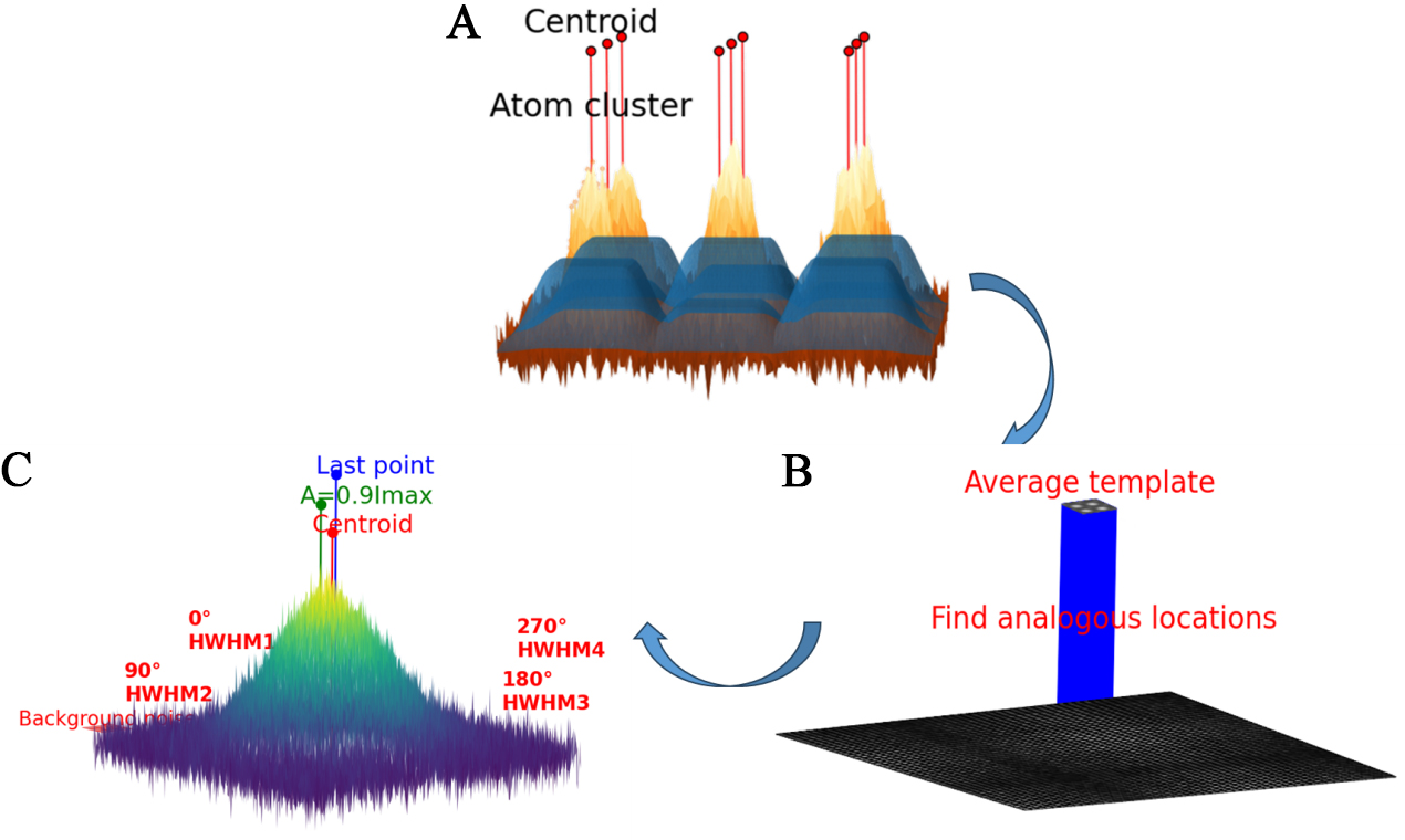
Figure 1. Schematic representations of the three main algorithms. (A) Extraction of individual atomic clusters via an adaptivethreshold method, followed by application of the centroid method to each cluster to obtain preliminary atomic positions; (B) Generation of an average template and its use to locate matching positions within the raw image; (C) For each peak, extraction of Imax​, full width at halfmaximum (FWHM), background noise, and centroid coordinates to estimate all Gaussianfitting parameters, thereby yielding highprecision atomic coordinates. HWHM: Half width at half maximum.

Enhanced centroid method for atomic row localization algorithm
In the conventional centroid method, for a set of n d-dimensional vectors x_i = (x_i1, x_i2, …, x_id), the centroid C is defined as^[14]:

(1) $$ \boldsymbol{c}=\frac{1}{n} \sum_{i=1}^{n} \boldsymbol{x}_{i}=\left(\frac{1}{n} \sum_{i=1}^{n} x_{i 1}, \frac{1}{n} \sum_{i=1}^{n} x_{i 2}, \ldots, \frac{1}{n} \sum_{i=1}^{n} x_{i d}\right) \\ $$

For the application to STEM images, the vectors are typically the three-dimensional coordinates of the image pixels, denoted as^[14]

(2) $$ \mathbf{x}_{i}=\left(x_{i}, y_{i}, z_{i}\right) \\ $$

where x_i and y_i represent the pixel positions and z_i denotes the pixel contrast. In practical data processing, it is common to use the x_i and y_i coordinates as the fitting components while employing the contrast z_i as the weight for each pixel.

Therefore, for each atomic column in the STEM image, the fitting region (denoted as Ω) in the conventional centroid method is defined by the following equation^[14]:

(3) $$ \mathbf{c}=\frac{\sum_{\left(x_{i}, y_{i}\right) \in \Omega} f\left(x_{i}, y_{i}\right) \mathbf{x}_{i}}{\sum_{\left(x_{i}, y_{i}\right) \in \Omega} f\left(x_{i}, y_{i}\right)}=\left(\frac{\sum_{\left(x_{i}, y_{i}\right) \in \Omega} z_{i} x_{\mathrm{i}}}{\sum_{\left(x_{i}, y_{i}\right) \in \Omega} z_{i}}, \frac{\sum_{\left(x_{i}, y_{i}\right) \in \Omega} z_{i} y_{\mathrm{i}}}{\sum_{\left(x_{i}, y_{i}\right) \in \Omega} z_{i}}\right) \\ $$

However, in image processing, different regions are typically governed by a combination of features such as texture, color, brightness, and gradient. When these features exhibit significant heterogeneity in their distributions, traditional centroid methods - which rely solely on the mean value of features to represent class centers - may fail to adequately capture the intrinsic characteristics of each class^[15]. This limitation can adversely affect clustering accuracy and robustness. In grayscale STEM images, such heterogeneity primarily arises from variations in brightness across different regions. As a result, the problem transforms into the following: conventional centroid approaches often struggle to define an optimal fitting region for each atomic column - one that captures the main signal of the column without interference from neighboring columns - particularly under conditions of non-uniform background thickness or image noise. To address this, thresholding techniques are typically employed. The most basic thresholding method involves selecting a fixed threshold and comparing each pixel value against it. However, in images with substantial brightness variation between regions, fixed thresholds are often inadequate. In such cases, adaptive thresholding becomes necessary to ensure accurate segmentation. Therefore, the present software introduces an enhanced centroid method, developed on the basis of traditional centroid algorithms, specifically tailored to improve atomic column localization in complex STEM imaging conditions.

The core of the algorithm is to establish an adaptive threshold matrix. The idea is to first identify a neighborhood for each pixel (x_i, y_i) in the image, then perform local statistical analysis on that neighborhood, and finally compute the adaptive threshold A_ij at (x_i, y_i) based on a user-defined sensitivity parameter k with values ranging between 0 and 1 (where 1 corresponds to the minimum threshold and 0 to the maximum threshold)^[11]. Next, the specific implementation methods are described in detail.

To further expedite the computational process, the entire image is first converted into its integral image II (x, y) and its integral squared image II² (x, y)^[16]:

(4) $$ I I(x, y)=\sum_{i=0}^{x} \sum_{j=0}^{y} I_{i j} \\ $$

(5) $$ I I(x, y)=\sum_{i=0}^{x} \sum_{j=0}^{y} I_{i j} \\ $$

In this context, I_ij denotes a grayscale image normalized within the range [0, 1]. Subsequently, the integral image allows us to efficiently identify a 9 × 9 neighborhood for each pixel (x_i, y_i). Owing to the advantages of the integral image, it is sufficient for each neighborhood to locate only the coordinates of the upper-left corner (x_i1, y_i1) and the lower-right corner (x_i2, y_i2)^[17,18]:

(6) $$ x_{i 1}=\max \left(x_{i}-4,0\right), y_{i 1}=\max \left(y_{i}-4,0\right) \\ $$

(7) $$ x_{i 2}=\min \left(x_{i}+4, W-1\right), y_{i 2}=\min \left(y_{i}+4, H-1\right) \\ $$

Here, W and H represent the width and height of the image, respectively. Subsequently, the integral image is utilized to compute the local statistical measures. Firstly, for each local neighborhood, the pixel sum S_ij and the sum of squared pixel values S_2ij are calculated as follows^[17,18]:

(8) $$ S_{i j}=I I\left(x_{i 2}, y_{i 2}\right)-I I\left(x_{i 1}-1, y_{i 2}\right)-I I\left(x_{i 2}, y_{i 1}-1\right)+I I\left(x_{i 1}-1, y_{i 1}-1\right) \\ $$

(9) $$ H_{2}=2 H^{+}+2 e^{-} $$

For each 9 × 9 window, which contains a total of 81 pixels, the local mean m_ij, the local variance σ²_ij, and the local standard deviation s_ij can be computed as follows^[17,18]:

(10) $$ m_{i j}=\frac{S_{i j}}{81} \\ $$

(11) $$ \sigma^{2}{ }_{i j}=\frac{S_{2 i j}}{81}-m_{i j}{ }^{2} \\ $$

(12) $$ s_{i j}=\sqrt{\sigma^{2}{ }_{i j}} \\ $$

Finally, by combining the local statistical parameters with the user-selected threshold κ, we derive the following adaptive threshold formula^[11]:

(13) $$ A_{i j}=m_{i j}\left[1+k\left(s_{i j}-1\right)\right] \\ $$

Once the adaptive threshold matrix A_ij is obtained, regions where (I_ij - A_ij ≤ 0) an be masked. This process transforms each atomic column into an atomic cluster, which can be regarded as an “island”. Each “island” serves as our summation region. By combining this approach with the traditional centroid method, we can further derive an improved formula for the centroid method; specifically, Equation (14) is derived from Equations (3) and (13):

(14) $$ C_{x}=\frac{\sum_{i} \sum_{j} x_{i}\left(I_{i j}-A_{i j}\right)}{\sum_{i} \sum_{j}\left(I_{i j}-A_{i j}\right)}, C_{y}=\frac{\sum_{i} \sum_{j} y_{j}\left(I_{i j}-A_{i j}\right)}{\sum_{i} \sum_{j}\left(I_{i j}-A_{i j}\right)} \\ $$

The centroid coordinates obtained via this method can be considered as the initial positions of the atomic columns, which are subsequently refined using further Gaussian fitting. Notably, its adaptivethresholding scheme renders the method agnostic to material periodicity, enabling analyses that periodicitydependent tools like OO Picker cannot perform. The schematic of these algorithms is shown in Figure 1A.

However, due to thresholding, very weak scattering atomic column sites, such as oxygen atoms, may be lost. To recover these points, the software additionally incorporates a supplementary template matching module.

Rapid identification of weak scattering atomic columns via normalized cross-correlation
The Normalized Cross-Correlation (NCC) method is employed to locate the positions of weak scattering atomic columns. Initially, an atomic row is selected as a template, which is then utilized to generate a correlation map. This approach has proven to be highly effective in accurately determining the positions of weak scattering atomic columns. After each iteration, the user is required to designate templates from three distinct locations within the image. The correlated atomic positions are then aligned based on cross-correlation calculations using the templates selected from these three different atomic positions by the user^[19]:

(15) $$ C\left(T_{i}, T_{j}\right)=\sum_{x, y} T_{i}(x, y) \cdot T_{j}(x+\Delta x, y+\Delta y) \\ $$

where T_i and T_j are both pre-designated templates. Δx, Δy are displacement parameters determined by maximizing the cross-correlation value to achieve optimal alignment^[19]. Subsequently, an average template is generated by performing a pixel-wise average of the three aligned templates. This step is crucial for accurately locating atomic positions in high-resolution microscopic images of interfaces. It is noteworthy that, in certain cases, there may be multiple standard templates for determining atomic positions. In such scenarios, the process can be repeated multiple times to identify all relevant templates.

Once the templates are established, the cross-correlation map γ (u, v) determined using the following formula:

(16) $$ \gamma(u, v)=\frac{\sum_{x, y}\left[f(x, y)-\overset{\text{-}}{f}_{u, v}\right][t(x-u, y-v)-\overset{\text{-}}{t}]}{\left\{\sum_{x, y}\left[f(x, y)-\overset{\text{-}}{f}_{u, v}\right]^{2} \sum_{x, y}[t(x-u, y-v)-\overset{\text{-}}{t}]^{2}\right\}} \\ $$

where f represents the image, $$ \overset{\text{-}}{t} $$ is the mean of the template, and $$ \overset{\text{-}}{f}_{u, v} $$ denotes the mean of f (x, y) within the template region.

The cross-correlation map effectively amplifies weak signals, making them more discernible. Subsequently, the improved centroid method is utilized to accurately determine the position of each spot generated in the correlation map^[20,21]. The schematic of these algorithms is shown in Figure 1B.

Enhanced 2D Gaussian fitting
In STEM images, the intensity of atoms approximates the intensity distribution of Airy disks. The central intensity is indicative of the scattering strength of the electron beam at the atomic position. 2D Gaussian functions provide the most computationally efficient representation of Airy disks and exhibit minimal deviation from the actual Airy disk profiles in practical applications.

To achieve more precise determination of atomic positions, a 2D Gaussian fitting procedure is employed prior to finalizing the output results. This fitting process enhances the accuracy of the atomic localization by refining the initial positions obtained through centroid and cross-correlation methods. Traditional approaches to 2D Gaussian fitting include least-squares Gaussian iterative fitting, nine-point regression, and fast Fourier transform (FFT)-based methods. Among these, the least-squares Gaussian iterative fitting offers the highest precision; however, it is associated with significant computational costs and extended processing times due to its iterative nature. Conversely, methods such as nine-point regression and FFT-based fitting, while faster, do not achieve the necessary level of accuracy required for precise atomic localization^[22,23].

To balance accuracy and computational efficiency, optimization techniques based on least-squares Gaussian iterative fitting, such as iterative optimization, are typically employed. Nonetheless, these optimized methods tend to exhibit reduced robustness in the presence of noise, which can compromise the reliability of atomic position determination in noisy STEM images. Consequently, there is a continual need for the development of more efficient and robust 2D Gaussian fitting algorithms that can maintain high precision while mitigating the impact of noise.

Finally, the software adopts a method known as enhanced weighted overdetermined regression, which maintains precision comparable to least-squares Gaussian iterative fitting even at lower signal-to-noise ratios (SNRs), while achieving a speed increase of two orders of magnitude and demonstrating robustness against noise. The method is formulated as follows^[24]:

(17) $$ I_{x y}=A \cdot \exp \left[-\left(\frac{\left(x-x_{0}\right)^{2}}{2 \cdot w_{x}^{2}}+\frac{\left(y-y_{0}\right)^{2}}{2 \cdot w_{y}^{2}}\right)\right]+\varepsilon_{x y} \\ $$

where I_xy represents the pixel intensity, A is the peak amplitude, x and y denote the coordinates of an individual pixel, x₀ and y₀ are the coordinates of the Gaussian center obtained initially via the centroid method, w_x and w_y is the standard deviation or width of the Gaussian distribution, and ε_xy corresponds to the noise^[24].

Nevertheless, this approach has inherent limitations. Its most significant drawback is the requirement for relatively accurate initial coordinates and a set of parameters - such as peak intensity, the standard deviation (or width) of the Gaussian distribution, and background noise - which is common to all 2D Gaussian fitting algorithms. Typically, users must manually input and adjust these parameters to obtain sufficiently precise values. In STEM images containing hundreds or thousands of 2D Gaussian distribution points with varying characteristics, identifying parameter values that ensure convergence for all points is particularly challenging, making the process time-consuming and demanding considerable patience and expertise. This challenge has motivated subsequent improvements in the methods for preliminary fitting parameter estimation. To streamline the process while ensuring optimal fitting for each atom, the software presets these parameters automatically. Considering the influence of noise, the maximum intensity of the Gaussian distribution is typically set slightly higher than the peak intensity. Therefore, A is set to 90% of the maximum contrast I_max within the fitting region. The standard deviation or width w_x and w_y is automatically estimated using the full width at half maximum (FWHM) method, approximated by $$ w \approx \frac{\mathrm{FWHM}}{2.355}$$, where FWHM is the distance between two symmetric points corresponding to half the peak height, determined via interpolation. To estimate the noise ε_xy, a background region statistics method is employed. For each point, the software automatically searches for a region within two to four w units away from the initially estimated centroid position. It identifies the area with the lowest average intensity, presumed to be an information-free region, and calculates the standard deviation of the intensity within this region to estimate the background noise. For the final fitting region, a width of w is selected. This approach ensures that, even in STEM images with significant background noise fluctuations, the parameters can be individually adjusted for each atom. Consequently, the overdetermined nature of the fitting process for all atoms results in more precise coordinates, effectively replacing the initial estimates with highly accurate atomic positions. The schematic of these algorithms is shown in Figure 1C.

Steps of analysis

The software is developed using the MATLAB (M) programming language and is organized into several distinct modules, as illustrated in the flowchart of Figure 2. The user interface of the software is depicted in Figure 3.

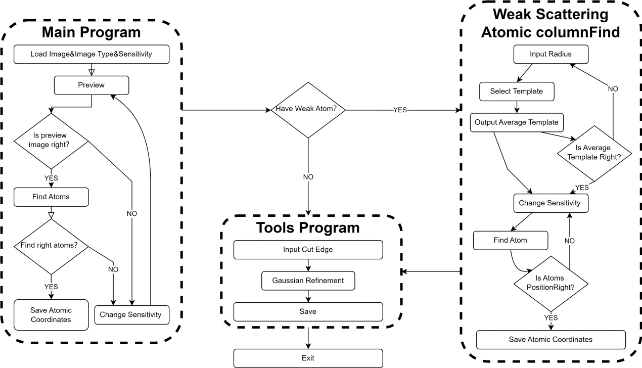
Figure 2. Workflow diagram of software usage. The software consists of three main components: the main program, the weak scattering atomic columns find program, and the Tools program. The Main program is executed first, followed by the selective use of the weak scattering atomic columns find program as needed, and finally, the tools program is employed.

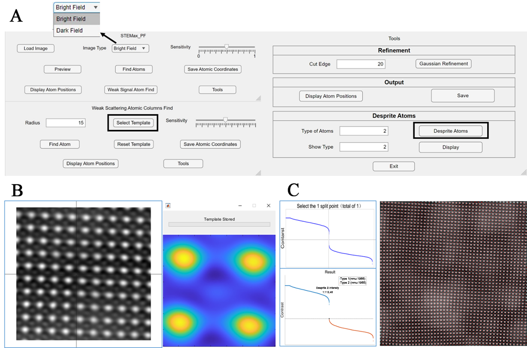
Figure 3. Schematic diagram of the software interface. (A) Interface pages for the three main programs; (B) Operational interface after clicking the “Select Template” button, where users sequentially select three templates using the crosshair; (C) Operational interface after clicking the “separate atoms” button, allowing users to categorize atoms by contrast into desired types and view the positions of atoms in each category.

The workflow begins by launching the main program of STEMax_PF and utilizing the ”Load Image” script to import images. The software supports a variety of mainstream image formats, including JPEG, PNG, BMP, and TIFF. Given that the primary application of this software targets STEM images, it additionally supports the simultaneous reading of DM3 and DM4 file formats and outputs the actual size of each pixel in the image^[25]. Users have the option to select between HAADF images and annular bright field (ABF) images, with support for both modalities, as shown in the enlarged figure in Figure 3A. Subsequently, by selecting an appropriate threshold, the software separates each atomic cluster. This step is verified through the “Preview” function, which employs the enhanced centroid method to determine and save the positions of atoms.

The “weak scattering atomic columns find” script is designed to identify atoms with very weak intensities that could not be detected in the initial step. If no such atoms are present, this script can be skipped. During this process, users are required to select three templates of identical size, with the template size determined by the “radius” parameter. Based on the average of these three templates, the software identifies similar regions within the image, thereby locating atoms with very weak intensities. The specific page is shown in the Figure 3B. This approach necessitates that the templates contain information about different types of atoms, allowing the software to determine the positions of extremely weakly intense atoms by leveraging the positional relationships between different types of atoms.

Upon obtaining satisfactory atomic positions, the final processing is conducted using the “tools” script. Users can select an appropriate “cut edge” option to truncate incomplete lattice regions at the edges of the image, followed by Gaussian fitting. In comparison to other widely used software packages^[4,5], STEMax_Peaks does not require the selection of initial parameters, as it can automatically estimate the initial fitting values for each atom. This significantly reduces the complexity of the operation. It is important to note that during the initial use, the software necessitates the configuration file to initiate a parallel pool (parpool). This setup process takes approximately a few minutes but is justified by the substantial performance gains achieved. MATLAB’s built-in Parallel Computing Toolbox enhances the speed of Gaussian fitting by an order of magnitude. Finally, the “save” button allows users to save all atomic information, including the X and Y coordinates and intensities of atoms, in a TXT file format within the directory of the first image loaded.

When calibrating multiple types of atoms simultaneously, the software also provides a distinguishing function. It will plot the contrast for all atoms, and subsequently allow the user to separate different atoms based on the numerical input of “types of atoms”. The positions of each type of atom can then be viewed using the “display” function below. The information of different types of atoms is also stored in separate TXT files, facilitating detailed structural analysis. The specific page is shown in the Figure 3C.

Compared to commonly used open-source software such as Atomap, our software significantly reduces the complexity of operation. All tasks can be executed through the interface depicted in Figure 3, with immediate feedback provided at every stage. Users can quickly calibrate parameters using simple mechanisms such as sliding controls and numerical input adjustments, thereby considerably lowering the entry threshold and enhancing the user experience. This design enables researchers to dedicate more time to data analysis and scientific investigation rather than to complex parameter tuning and algorithm selection.

Experimental section

The preparation of STEM samples followed standard protocols, encompassing wire cutting, mechanical grinding, polishing, pitting grinding, and argon ion beam milling under liquid nitrogen cooling. Prior to conducting STEM experiments, the samples underwent plasma cleaning for 30 min in an argon atmosphere using an EC-52000IC plasma cleaner. This step was essential to eliminate surface contamination from hydrocarbons. STEM investigations were performed using a JEM-ARM300F2 (Grand ARM) scanning transmission electron microscope.

During the STEM experiments, the rapid scanning direction was aligned parallel to the horizontal axis of the resulting images. To enhance the SNR of the HAADF and ABF images and to minimize image distortion, a sequence of 10 frames was continuously captured with short dwell times. The frame sequences were subsequently aligned using the Gatan image alignment plugin, “SmartAlign”, within the digital micrograph software. This alignment process included diagnosing and correcting for sample drift between frames for both HAADF and ABF images, effectively removing drift-induced artifacts. Moreover, summing multiple frames can effectively enhance the signal, thereby preserving the material’s unique properties.

Following alignment, the frames were overlaid to construct a composite image with improved SNR and reduced distortions. The resulting STEM images were further processed for noise reduction using the Radial Wiener Filter plugin available in Digital Micrograph. This denoising step ensured the clarity and accuracy of the atomic-scale features observed in the final images.

By adhering to these meticulous preparation and imaging procedures, the software-averaged STEM images achieved high precision and reliability, facilitating detailed analysis of complex material systems.

Method accuracy and precision

To validate the accuracy of the software, specifically designed simulated images were generated for verification purposes. The simulation diagram is presented in Figure 4A. In these simulated images, a 50 × 50 array of A-site atoms with high intensity and a perfect lattice structure was first created. Subsequently, B-site atoms were simulated to represent the [100] crystallographic phase of the perovskite ABO₃ structure within STEM images and were inserted between the A-site atoms. For the Bsite atoms, those in the upper half of the image are shifted by one pixel toward the left-up direction (135°), while those in the lower half are shifted by one pixel toward the right-down direction (315°). These positional shifts emulate different orientations of ferroelectric domains. In the generated images, each pixel corresponds to an actual size of 1 pixel = 5.49 pm^[26]. For the Bsite atoms, those in the upper half of the image are shifted by one pixel toward the northwest (135°), while those in the lower half are shifted by one pixel toward the southeast (315°).

Figure 4. Simulation of HAADF images with B-site/A-site intensity at 10% of A-site/B-site intensity of perovskite ABO₃, e.g., ferroelectric LaAlO₃ or NaNbO₃, and SNR values of 50, 15, and 5 to validate precision. (A) Schematic of a simulated 50 × 50 image and enlarged views of a single lattice for SNR values of 50, 15, and 5; (B) Average templates obtained using the Cross-Correlation method for images with different SNRs; (C) Final point detection results for images with varying SNRs; (D) Schematic illustration of atomic displacements measured by the software at the simulated interface for images with different SNRs, with the color bar indicating colors corresponding to different displacement directions; (E) Scatter plots of the differences between measured displacements and theoretical displacements for images with different SNRs, where the distance from the origin represents the Euclidean distance and the standard deviation indicates precision. HAADF: High-angle annular dark-field; SNR: signal-to-noise ratio. SD: standard deviation.

Since the variance of Poisson noise is equal to the mean of the signal, the brightness of the image was first normalized. Subsequently, the brightness was adjusted so that its mean equals (SNR)^2[25]. Random noise was then introduced using a Poisson distribution, thereby generating Poisson noise. Simulated images with SNRs of 5, 15, and 50 were produced to validate the software’s performance; different SNRs exert varying effects on the signal, as illustrated in Figure 4B. Poisson noise is the predominant noise source in STEM imaging, thereby effectively simulating the noise present in actual STEM images^[28,29]. According to the study by Bals et al., the precision in image measurements was defined as the standard deviation of the measured displacement distances^[30].

The final atomic positions and their corresponding displacement images are illustrated in the accompanying figure. To quantify the deviation between the obtained displacements and the theoretical displacements, the Euclidean distance was employed. The advantage of using Euclidean distance lies in its ability to comprehensively reflect both the directional and magnitude components of the deviation. This metric allows for an effective comparison with the Gaussian-distributed displacements introduced by varying SNRs, thereby accurately representing the final displacement errors.

The precision of the software was validated using specifically generated simulated images. Testing was conducted on a computer without a graphics processing unit, equipped with an Intel® Core^TM i5-8400 CPU running at 2.80 GHz and 7.8 GB of RAM. By initiating eight parallel pools for computation, Gaussian fitting for approximately 5,000 atoms was completed in approximately 36 s. Notably, this hardware configuration is considered relatively outdated, indicating that the software is capable of processing nearly all STEM images on almost any standard computer.

Initially, as can be seen from Figure 4, the precision of the proposed method was compared across different SNRs, with the intensity of B-site atoms set to 10% of that of A-site atoms, a condition that is relatively rare in real-world scenarios. We deliberately made this choice in order to evaluate our software under the most challenging conditions. It is important to emphasize that achieving a tenfold contrast difference between the A-site and B-site atoms in HAADF images is extremely demanding in real materials. This strict requirement can only be met in specific perovskite systems where the atomic number (Z) ratio between the A- and B-site elements exceeds at least 3:1. Exemplary systems include NaNbO₃ (A-site: Na, Z = 11; B-site: Nb, Z = 41), LaAlO₃ (A-site: La, Z = 57; B-site: Al, Z = 13), NdAlO₃ (A-site: Nd, Z = 60; B-site: Al, Z = 13), etc. Although materials satisfying this condition are relatively rare, their scarcity makes them an ideal test bed for validating our method under extreme contrast conditions. Moreover, the rigor of these conditions serves to underscore the broad applicability of our software. The final statistical results are presented below.

Figure 4A displays the simulated images, magnified lattice structures, and Figure 4B-D shows the effectiveness of template matching when locating B-site atoms, zoomed-in views of point-finding results, and zoomed-in views of polarization effects. The color bar on the right corresponds to polarization in various directions. Figure 4E presents an error analysis, wherein the X and Y coordinates in the scatter plot represent the deviations of the measured polarization from the theoretical polarization in the X and Y directions, respectively. The distance from each point to the origin of the coordinate axes quantifies the error, measured in picometers (pm).

The results revealed that for images with an SNR of 5, the standard deviation of all displacement Euclidean distances was 0.827 pixels; for an SNR of 15, it was 0.423 pixels; and for an SNR of 50, it was 0.206 pixels. Considering that the simulated image scale is 1 pixel = 5.49 pm, the corresponding precisions of the method are 4.5418 pm, 2.3267 pm, and 1.1326 pm for SNRs of 5, 15, and 50, respectively. These findings demonstrate that the software consistently achieves precision at the single-picometer level across varying SNRs. This high level of precision, even at lower SNRs, underscores the software's robustness and its suitability for detailed analysis of STEM images under diverse experimental conditions.

Furthermore, we observed a pronounced preferred direction in the bias at an SNR of 15, and slight orientation biases were also present at SNR values of 5 and 50. We think that under the same SNR, the noise associated with strong atoms at position A is significantly higher than that for the weaker atoms at position B. In cases of very weak peaks, if a B atom tends to approach an A atom from a specific direction - particularly when it is closer to one side, as illustrated in our displacement scenario - the noise contributions from the A atoms in the four surrounding directions can induce a slight asymmetry in the background fitting. This effect only becomes evident when the B peak is extremely weak. When the SNR is low, the elevated noise levels obscure these subtle asymmetries; conversely, at very high SNRs, the noise is too minimal to generate any significant asymmetry. Consequently, this directional bias is most apparent at an SNR of 15, whereas it is less pronounced at SNR values of 5 or 50.

Subsequently, the proposed method was compared with commonly employed traditional calibration techniques, utilizing both commercial software and the software developed by Mitchell^[31], including the centroid method and 2D Gaussian fitting. Experimental findings revealed that for B-site atoms with extremely weak intensities - for instance, when B-site atom intensity is set to 10% of that of A-site atoms - traditional methods fail to accurately determine atomic positions. Therefore, to facilitate comparison under different SNRs and methods, the intensity of the B-site atoms was increased to 50% of that of the A-site atoms. Figure 5A shows the magnified atomic lattice. Figure 5B presents the detailed experimental results regarding precision. In the scatter plot, the X and Y coordinates denote deviations between the measured displacement and the theoretical polarization in each respective direction, while each point’s distance from the coordinate origin quantifies the error in pm. The results indicate that at an SNR of 5, the centroid method attains a precision of 4.3217 pm, the 2D Gaussian method achieves 2.2355 pm, and the proposed software yields 2.3782 pm. At an SNR of 15, the centroid method offers a precision of 2.6851 pm, the 2D Gaussian method 1.2589 pm, and the proposed software 1.2846 pm. At an SNR of 50, the centroid method attains a precision of 1.9797 pm, the 2D Gaussian method 1.1076 pm, and the proposed software 1.1897 pm. Figure 5C employs a radar chart to illustrate the precision, processing speed, and robustness of the three methods. Different colors represent different methods. Precision is quantified by taking the reciprocal of the average precision measured under various SNR conditions (in units of pm^-1). Robustness is represented by the reciprocal of the standard deviation of the precision under the same conditions (also in units of pm^-1). Speed is conveyed by the reciprocal of the processing time (in units of s^-1). As shown in the figure, the proposed software achieves roughly half the processing speed of the centroid method, yet both methods are two orders of magnitude faster than the 2D Gaussian method. At the same time, the precision and noise robustness of the proposed software are close to those of the 2D Gaussian method, clearly demonstrating its advantages.

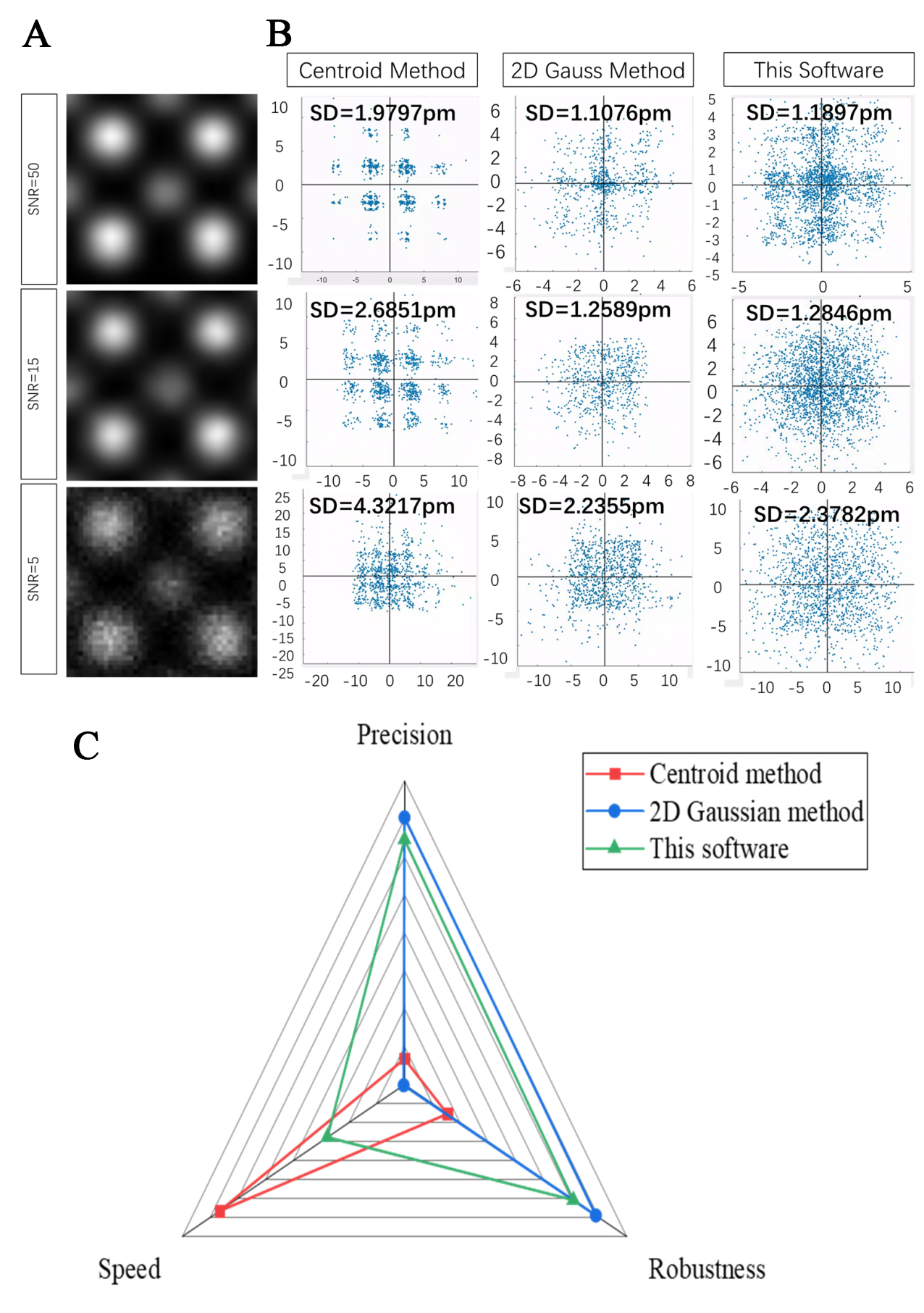
Figure 5. Simulation of HAADF images with B-site intensity at 50% of A-site intensity. (A) Enlarged views of a single lattice for SNR values of 50, 15, and 5; (B) Comparison of measurement precision among the proposed software, the centroid method, and the 2D Gaussian fitting method under SNR values of 50, 15, and 5, illustrated by scatter plots of the differences between the observed and theoretical displacements; (C) Radar map comparing the three methods in terms of speed, precision, and robustness. HAADF: High-angle annular dark-field; SNR: signal-to-noise ratio; 2D two-dimensional.

Additionally, it was found that the centroid method exhibited clustering at fixed symmetrical positions, likely due to the influence of noise introduced by the fixed pattern on the centroid calculations.

The simulated images used in this study do not account for scanning noise, as most low-frequency scan distortions can be effectively corrected using the “SmartAlign” procedure applied in the experimental section. In cases where such correction is not performed, the accuracy of this software may be reduced due to inherent limitations of the Gaussian fitting algorithm.

We plan to extend our software in future updates by incorporating a module for generating distortion-corrected images, in order to further enhance the accuracy and universality of our analysis.

These results demonstrate that the proposed software significantly outperforms the centroid method in terms of precision and maintains only a minor difference in precision compared to the 2D Gaussian method. Furthermore, at higher SNR levels, the precision gap between the proposed method and the 2D Gaussian method even decreased, potentially because the software individually estimates fitting parameters for each atom, thereby reducing the impact of varying peak intensities among different atoms. When compared to the precision achieved for simulated images of weak scattering B-site atoms, it was observed that although there is a reduction in precision under extremely weak signal conditions (where the peak intensity of the Gaussian distribution is very low), the method still maintains precision at the picometer level.

Potential applications

In addition to the ABO₃ perovskite structure image peak detection discussed in previous studies, this software can also be utilized to locate atomic positions in specialized structures.

For certain specialized materials, the presence of difficult-to-identify atoms is common. These atoms may exhibit extremely weak signals or occupy closely adjacent positions, resulting in numerous atoms within a single image that are challenging to detect directly. In such cases, the ‘Weak Scattering Atomic Columns Find’ script of the software can be employed to assist in the calibration process.

In this study, we selected a structure known as anti-fluorite, a highly complex cubic phase. Its structural diagram is illustrated in Figure 6A. For this structure, Figure 6B presents a STEM image acquired along the [110] crystallographic zone axis, it is evident that within each column of atoms situated between two strong scattering atomic columns, there are four atoms with relatively weaker intensities. However, due to the proximity of two of these weaker atoms to the strong scattering atomic columns and the limitations imposed by atomic distance and signal intensity, conventional calibration methods struggle to accurately determine the positions of all four atoms while maintaining precision, as illustrated in Figure 6C^[32]. This often results in missing peaks and superfluous peaks. In contrast, the proposed software overcomes this challenge by establishing two independent templates, as shown in Figure 6D, enabling the accurate calibration of all four weak scattering atomic columns. The final calibration results presented in Figure 6E demonstrate that the software successfully identifies the positions of all four weak scattering atomic columns without introducing any extraneous or erroneous atoms. This capability highlights the software’s effectiveness in calibrating atoms within materials that present significant calibration difficulties.

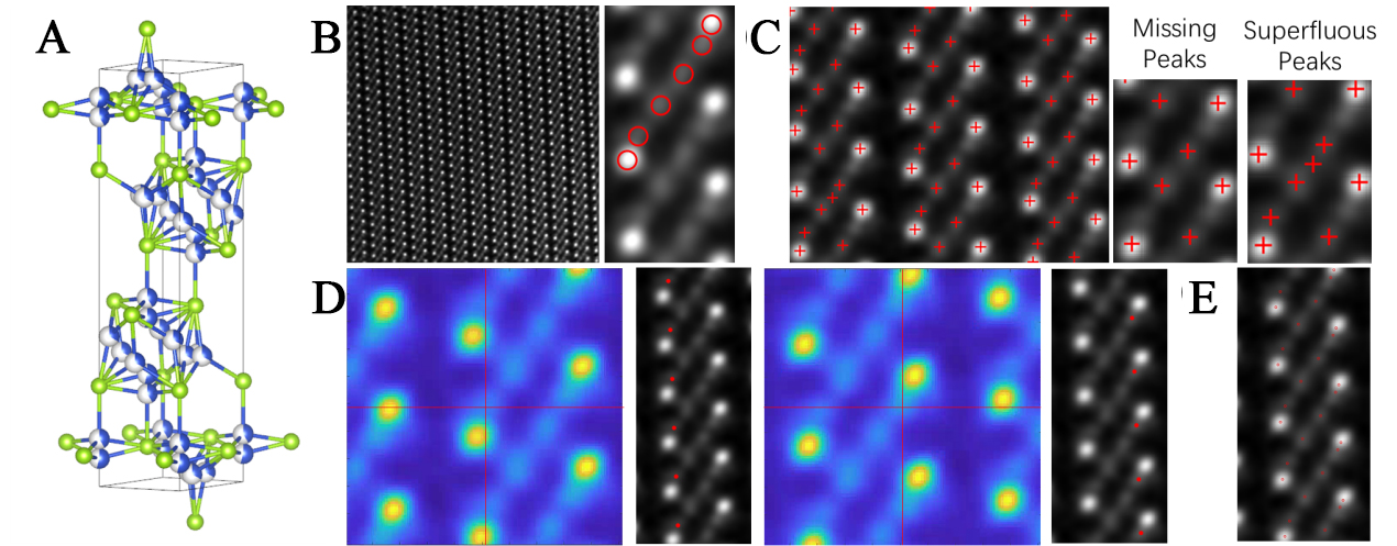
Figure 6. Illustration of the software’s template-based point detection performance for atoms with extremely weak signals. (A) Structure of anti-fluorite; (B) STEM image of the material and its structural schematic; (C) Point detection results obtained using Tempas, displaying missing peaks and superfluous peaks; (D) Effectiveness of template selection within the software; (E) Final point detection outcomes. STEM: Scanning transmission electron microscopy.

REFERENCES

1. Pennycook, S. J.; Jesson, D. E. High-resolution incoherent imaging of crystals. Phys. Rev. Lett. 1990, 64, 938-41.
2. Pennycook, S.; Jesson, D. Atomic resolution Z-contrast imaging of interfaces. Acta. Metallurgica. et. Materialia. 1992, 40, S149-59.
3. Qu, W.; Zhao, Z.; Yang, Y.; et al. Atomic-level quantitative analysis of electronic functional materials by aberration-corrected STEM. Chinese. Phys. B. , 33, 116802.
4. Wang, Y.; Salzberger, U.; Sigle, W.; Eren, Suyolcu. Y.; van, Aken. P. A. Oxygen octahedra picker: a software tool to extract quantitative information from STEM images. Ultramicroscopy 2016, 168, 46-52.
5. Nord, M.; Vullum, P. E.; MacLaren, I.; Tybell, T.; Holmestad, R. Atomap: a new software tool for the automated analysis of atomic resolution images using two-dimensional Gaussian fitting. Adv. Struct. Chem. Imag. 2017, 3, 9.
6. Rekik, A.; Zribi, M.; Benjelloun, M.; ben, Hamida. A. A k-Means clustering algorithm initialization for unsupervised statistical satellite image segmentation. 2006. 1ST. IEEE. International. Conference. on. E-Learning. in. Industrial. Electronics. , IEEE Publishers, Piscataway, New Jersey, USA, 2006; pp 11-6.
7. Boyat, A. K.; Joshi, B. K. A review paper: noise models in digital image processing. arXiv: arXiv:1505.03489v1 [Preprint]. 2015 [cited 2017 Feb 9]: [13 p.]. Available from: https://doi.org/10.48550/arXiv.1505.03489.
8. Cheezum, M. K.; Walker, W. F.; Guilford, W. H. Quantitative comparison of algorithms for tracking single fluorescent particles. Biophys. J. 2001, 81, 2378-88.
9. Lin, R.; Zhang, R.; Wang, C.; Yang, X. Q.; Xin, H. L. TEMImageNet training library and AtomSegNet deep-learning models for high-precision atom segmentation, localization, denoising, and deblurring of atomic-resolution images. Sci. Rep. 2021, 11, 5386.
10. Nan, H.; Lu, L.; Ma, X. Application of sliding window algorithm with convolutional neural network in high-resolution electron microscope image. J. Chin. Electr. Microsc. Soc. 2021, 40, 242-50. (in Chinese).
11. Bradley, D.; Roth, G. Adaptive thresholding using the integral image. J. Graphics. Tools. 2007, 12, 13-21.
12. Okunishi, E.; Ishikawa, I.; Sawada, H.; Hosokawa, F.; Hori, M.; Kondo, Y. Visualization of light elements at ultrahigh resolution by STEM annular bright field microscopy. Microsc. Microanal. 2009, 15, 164-5.
13. Born, M.; Wolf, E. Principles of Optics: Electromagnetic Theory of Propagation, Interference and Diffraction of Light, 7th ed.; Cambridge University Press; 1999.
14. Hu, M. K. Visual pattern recognition by moment invariants. IRE. Trans. Inf. Theory. 1962, 8, 179-87.
15. Sneath, P. H. A. Numerical Taxonomy (by) Peter H.A. Sneath (and) Robert R. Sokal: The Principles and Practice of Numerical Classification; W.H. Freeman and Company, 1973.
17. Lewis, J. P. Fast Template Matching. In Vision Interface 95, Proceedings of the Canadian Image Processing and Pattern Recognition Society, Quebec City, Canada; May 15-19, 1995; Canadian Image Processing and Pattern Recognition Society: Québec, Canada, 1995; pp 15-9.http://scribblethink.org/Work/nvisionInterface/vi95_lewis.pdf (accessed 2025-11-26).
18. Shafait, F.; Keysers, D.; Breuel, T. M. Efficient implementation of local adaptive thresholding techniques using integral images. In IS&T/SPIE International Symposium on Electronic Imaging, Proceedings of the 15th Conference on Document Recognition and Retrieval, San Jose, USA; January 26-31, 2008; SPIE: San Jose, USA, 2008; pp 681510.
19. Frank, J.; Goldfarb, W.; Eisenberg, D.; Baker, T. S. Reconstruction of glutamine synthetase using computer averaging. Ultramicroscopy 1978, 3, 283-90.
20. Lewis,JP. Fast normalized crosscorrelation. San Rafael, CA: Industrial Light & Magic; 1995. https://www.researchgate.net/publication/2378357_Fast_Normalized_Cross-Correlation (accessed 2025-6-4).
21. Shapiro, L. G. Computer and Robot Vision; Vol 2 Reading, MA: AddisonWesley Publishing Company, 1992.
22. Teukolsky, S. A.; Vetterling, W. T.; Flannery, B. P. Numerical Recipes: The Art of Scientific Computing, 3rd ed.; Cambridge University Press; 2007.
23. Nobach, H.; Honkanen, M. Two-dimensional Gaussian regression for sub-pixel displacement estimation in particle image velocimetry or particle position estimation in particle tracking velocimetry. Exp. Fluids. 2005, 38, 511-5.
24. Anthony, S. M.; Granick, S. Image analysis with rapid and accurate two-dimensional gaussian fitting. Langmuir 2009, 25, 8152-60.
25. Sigworth, F. Read .dm3 and .dm4 image files. MATLAB Central File Exchange. Accessed December 23, 2024. https://www.mathworks.com/matlabcentral/fileexchange/43005-read-dm3-and-dm4-image-files (accessed 2025-6-4).
26. Mitchell, D. R. G. Create a Synthetic HAADF Image. Version 20211129, v1.2 [Source code] http://dmscripting.com/create_a_synthetic_haadf_image.html (accessed 2025-6-4).
27. Bosman, M.; Keast, V. J.; García-Muñoz, J. L.; D'Alfonso, A. J.; Findlay, S. D.; Allen, L. J. Two-dimensional mapping of chemical information at atomic resolution. Phys. Rev. Lett. 2007, 99, 086102.
28. Mevenkamp, N.; Binev, P.; Dahmen, W.; Voyles, P. M.; Yankovich, A. B.; Berkels, B. Poisson noise removal from high-resolution STEM images based on periodic block matching. Adv. Struct. Chem. Imag. 2015, 1, 4.
29. Jones, L.; Nellist, P. D. Identifying and correcting scan noise and drift in the scanning transmission electron microscope. Microsc Microanal 2013;19:1050-60.
30. Bals, S.; Van, Aert. S.; Van, Tendeloo. G.; Avila-Brande, D. Statistical estimation of atomic positions from exit wave reconstruction with a precision in the picometer range. Phys. Rev. Lett. 2006, 96, 096106.
31. Mitchell, D. R. G. Atomic Displacement. Version 20230104, v2.1 [Source code] http://dmscripting.com/atomic_displacement.html (accessed 2025-6-4).
32. Total Resolution. *Tempas* (Version 3.0.42) [Software]. 2023. https://www.totalresolution.com/Tempas.htm.
Cite This Article
How to Cite
Download Citation
Export Citation File:
Type of Import
Tips on Downloading Citation
Citation Manager File Format
Direct Import: When the Direct Import option is selected (the default state), a dialogue box will give you the option to Save or Open the downloaded citation data. Choosing Open will either launch your citation manager or give you a choice of applications with which to use the metadata. The Save option saves the file locally for later use.
Indirect Import: When the Indirect Import option is selected, the metadata is displayed and may be copied and pasted as needed.
About This Article
Special Topic
Copyright
Data & Comments
Data
0
Comments
Comments must be written in English. Spam, offensive content, impersonation, and private information will not be permitted. If any comment is reported and identified as inappropriate content by OAE staff, the comment will be removed without notice. If you have any queries or need any help, please contact us at [email protected].