


Intelligent prediction of the remaining useful life of lithium-ion batteries based on a CGHF-MDH-Mamba model
 0
0 Abstract
Lithium-ion batteries are core components of renewable generation and energy-storage systems and are widely deployed in PV/wind grid scheduling and e-mobility. Accurate remaining useful life (RUL) prediction is essential for operational stability and cost control. This paper proposes a battery life prediction approach that integrates channel-grouping half-convolution (CGHF) and a monotonic decreasing head (MDH) within a Mamba-based sequence modeling framework. CGHF reduces computational redundancy while strengthening multi-scale temporal representations; the selective state-space module of Mamba efficiently captures long-range dependencies; MDH imposes an explicit “non-increasing capacity” constraint at the decoder to enhance robustness and interpretability. Experiments on the National Aeronautics and Space Administration (NASA) Randomized Battery Usage Dataset and the Tongji University (TJU) Commercial Lithium-Ion Battery Cycling Dataset demonstrate superior RUL accuracy, achieving minimum capacity-prediction mean absolute errors (MAEs) of 0.0081 and 0.0009 Ah, respectively, outperforming strong baselines under the same settings. The method improves accuracy while maintaining fast inference, suggesting potential applicability to online health monitoring and maintenance planning, subject to further validation under more diverse operating conditions.
Keywords
1. INTRODUCTION
Lithium-ion batteries offer high energy density, long cycle stability, and low self-discharge[1], making them the preferred power source for grid-scale energy storage and electric vehicles[2]. Their operational reliability directly affects the safety and economic performance of downstream systems. Artificial intelligence and digital twin technologies have been increasingly applied in intelligent battery management systems to enhance remaining useful life (RUL) prediction and lifecycle optimization[3]. However, during long-term charge-discharge cycles, degradation is driven by coupled multiphysics effects such as electrode structure deterioration and electrolyte decomposition. This process is highly nonlinear and time-dependent. The characteristic information is often hidden in the spatiotemporal evolution of multi-source monitoring data such as voltage, current, and temperature, which makes direct identification and modeling difficult[4]. At the same time, the prediction of RUL[5] still faces both theoretical and technical challenges. Capacity recovery, nonlinear degradation, and strong individual variation make mechanism-based modeling difficult. Data-driven approaches, although flexible, often suffer from weak spatiotemporal coupling, high noise sensitivity, and lack of physical constraints, which limits their generalization and reliability in practical applications[6]. Smart evolving fuzzy predictors optimized by firefly algorithms have been proposed to improve adaptability and robustness under noisy degradation conditions[7]. Therefore, achieving accurate, efficient, and physically consistent RUL prediction has become a key scientific challenge in the health management of modern energy storage systems.
Current methods for lithium-ion battery RUL prediction can be divided into two main categories: model-based and data-driven[8,9]. Model-based methods describe degradation through electrochemical mechanisms or equivalent circuit models. For instance, the interactive multiple model particle flow filter (IMM-PFF) multi-model fusion method adapts to multi-stage degradation[2], and Gaussian mixture resampling improves particle filtering to reduce uncertainty[10]. However, these methods rely heavily on prior physical assumptions and show weak generalization under complex or unseen conditions such as those in photovoltaic or wind power systems, making them unsuitable for dynamic storage environments[11]. Data-driven methods have progressively improved in feature fitting. GRU-based frameworks combined with feature selection and clustering have further improved SOH and RUL prediction performance[12]. Hybrid ensemble learning frameworks have also been proposed to enhance the stability and accuracy of RUL prediction[13]. Recent studies have shown that extracting health indicators from partial charging curves can effectively improve the accuracy and practicality of data-driven SOH and RUL estimation methods[14]. The discrete wavelet decomposition and support vector regression model (DWD-SVR)[15] and the general regression neural network optimized by gravity search algorithm and enhanced with extreme learning machine (GRNN-GSA-ELM)[16] have achieved progress in multi-scale fitting and small-sample robustness, while K-means clustering-random forest and particle swarm optimization-elastic net models optimize individual adaptability and feature selection[15]. Nevertheless, the nonlinear representation of multi-dimensional time series remains limited under traditional machine-learning frameworks. Improved Dempster-Shafer evidence theory has been applied to enhance multi-source information fusion in RUL prediction[17]. Deep learning techniques have substantially improved lithium-ion battery RUL prediction in recent years. Recurrent and hybrid architectures, including OOA-BiGRU[18], CEEMDAN-CNN-BiGRU[19], attention-based BiLSTM models[20], CEEMDAN-BiLSTM-Transformer[21], and 1D CNN-BLSTM frameworks[22], have demonstrated enhanced temporal feature extraction capability. Transformer-based and multi-scale architectures, such as dynamic convolution transformers[23], temporal convolution networks (TCN)[24], transfer-learning AE-LSTM[25], TransRUL[26], comparative Transformer frameworks[27], and hybrid Informer-LSTM models[28], further improve long-sequence representation and degradation-stage awareness. However, major drawbacks remain. Most models extract temporal and spatial features separately, failing to capture the coupling among voltage, current, and temperature. The absence of physical constraints may lead to prediction trajectories that violate the capacity degradation mechanism. In addition, large parameter counts result in high inference costs[29].
Despite substantial progress, three key challenges remain in lithium-ion battery RUL prediction. First, spatiotemporal coupling of multi-dimensional features is insufficient. Most models handle voltage, current, and temperature independently in the temporal dimension and merge them by simple concatenation[30], which fails to capture their dynamic relationships during degradation and leads to incomplete feature representations. Additionally, the prediction process lacks physical constraints. Many models rely purely on data fitting without embedding the fundamental physical law of irreversible capacity decay, resulting in unrealistic oscillations or increases in the predicted trajectories that contradict actual degradation behavior[31]. Finally, model efficiency and architecture innovation lag behind. Current deep-learning models are typically large and slow during inference, which restricts their use in real-time monitoring or edge deployment. Efficient architectures such as Mamba[32] and channel-grouped half convolution[33] have not yet been systematically applied to RUL prediction. Recent work has demonstrated that state space models (SSM) can effectively capture long-term degradation dependencies in early RUL prediction tasks[34]. Their potential advantages in long-sequence dependency modeling and computational efficiency have not been fully realized[35].
Overall, this study aims to improve the accuracy, efficiency, and physical consistency of lithium-ion battery RUL prediction. Unlike existing approaches that introduce isolated improvements, this work focuses on a task-oriented integration of multi-level feature modeling and physics-informed constraints. The main contributions are as follows.
• A unified CGHF-VSN-Mamba framework is proposed to jointly model channel-level, variable-level, and temporal dependencies, enabling effective spatiotemporal coupling of battery degradation signals.
• A channel-grouped half convolution combined with attention is designed to reduce redundancy while preserving informative features, forming a lightweight yet expressive representation mechanism.
• A monotonic decreasing head (MDH) with adaptive gating is introduced to embed physical degradation constraints directly into the prediction process, improving both reliability and interpretability.
These components are not simply combined, but structurally coordinated to address three core challenges simultaneously: feature redundancy, long-sequence modeling, and lack of physical consistency.
2. METHODS
2.1. Channel-grouping half-convolution
In lithium-ion battery operation data, different variables and channel dimensions contain multi-scale degradation patterns. To capture local temporal dynamics while maintaining computational efficiency, a channel-grouping half-convolution (CGHF) module is introduced, as illustrated in Figure 1.
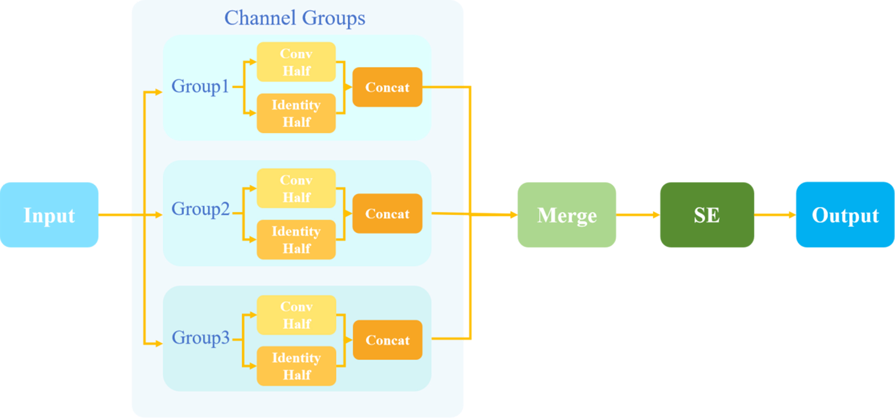
Figure 1. Structure of the CGHF module. CGHF: Channel-grouping half-convolution; SE: Squeeze-and-Excitation.
The key idea is to divide the input feature channels into several independent groups and use a “half-convolution plus half-bypass” structure within each group to achieve efficient modeling. Specifically, in each subgroup, half of the channels are processed by depth-wise separable convolution to extract local temporal features, while the remaining half are passed directly to preserve raw information. The two parts are then concatenated within the group and added to the input residual, balancing feature transformation and information fidelity.
Meanwhile, the CGHF module incorporates a Squeeze-and-Excitation (SE) attention mechanism[36]. This mechanism first performs global average pooling on each channel, then applies two fully connected layers with dimensionality reduction, expansion, and nonlinear activation to generate channel-wise weights. Finally, channel-wise reweighting is applied to the concatenated features, allowing the model to adaptively highlight channels more sensitive to capacity degradation while suppressing redundant or noisy information.
To balance local dynamic sensitivity and information fidelity, the input X ∈ ℝB×L×D is evenly divided into G groups. For the i- group, the channels are halved: one path passes through convolution, while the other bypasses to retain the original data. The two paths are concatenated within each group, groups operate in parallel, and SE attention performs the final channel recalibration.
The grouping and halving process are defined in Equation (1).
Here, X(i) denotes the output feature of the iii-th group. X(i)conv represents the half-channel feature processed by the depthwise convolution branch, while X(i)keep denotes the bypassed half-channel feature that preserves the original information. The in-group convolution extraction is defined in Equation (2).
In Equation (2),
The SE recalibration is defined in Equation (4).
In Equation (4), Y denotes the final output of the CGHF module after channel-wise recalibration. CatY(i) represents the concatenated features from all groups. W1 and W2 are the learnable weight matrices of the two fully connected layers in the SE attention, responsible for channel-wise dimensionality reduction and expansion.The resulting sigmoid activation generates channel weights that re-scale the concatenated features through Hadamard multiplication. Where Ø denotes GELU, BN denotes batch normalization, Conv1d denotes one-dimensional convolution, GAP denotes global average pooling, σ denotes the sigmoid function,
Compared with conventional convolutional structures, CGHF reduces redundancy through two mechanisms. First, the half-bypass design preserves raw features, avoiding excessive transformation that may amplify noise. Second, the SE attention dynamically suppresses channels with low contribution, ensuring that redundant information is not propagated to subsequent modules. This design is further complemented by the variable selection network (VSN) module at the variable level, forming a hierarchical redundancy reduction strategy.
2.2. VSN
In multivariate operation data, different features affect battery life to varying degrees. Treating all variables equally during prediction introduces feature redundancy and weakens the contribution of degradation-sensitive variables, thereby reducing both prediction accuracy and interpretability. To address this issue, the model incorporates a VSN that performs adaptive weighting and selection of input variables, as shown in Figure 2.
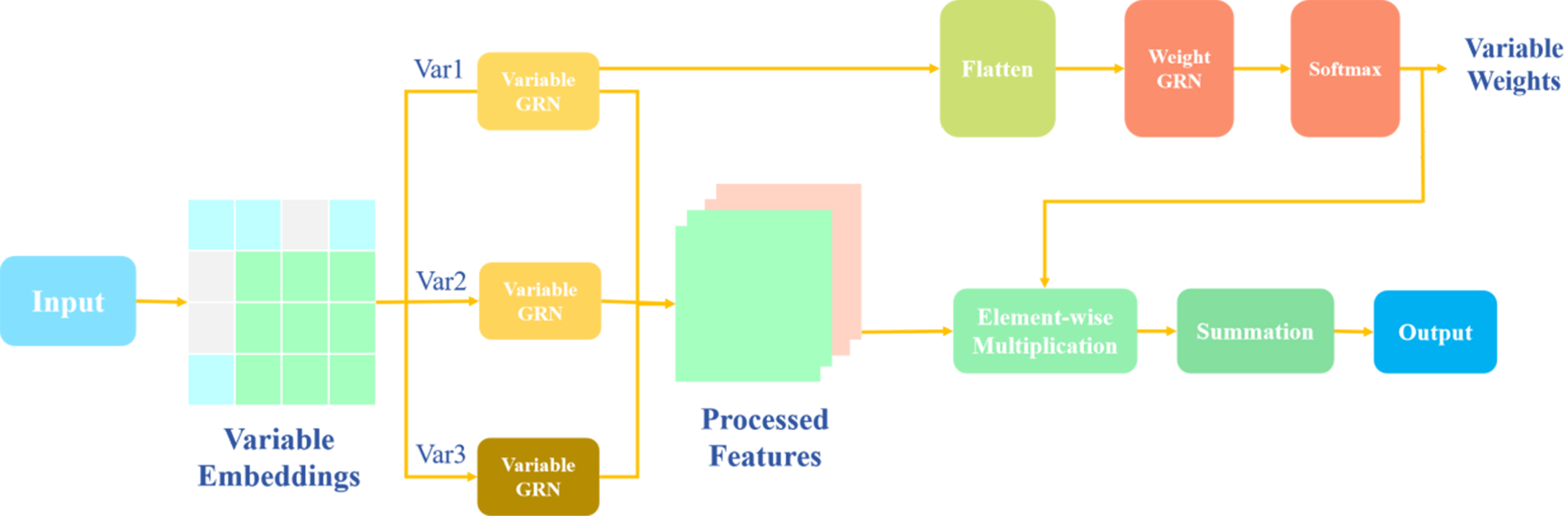
Figure 2. Structure of the VSN module. VSN: Variable selection network; GRN: gated residual network.
Specifically, the VSN constructs an independent gated residual subnetwork for each input variable to generate its candidate representation. This process ensures that every variable undergoes an independent nonlinear transformation before weighting, allowing the network to capture its latent temporal characteristics. Then, all candidate representations are concatenated and passed into a weight generation network, which applies a sparsified softmax distribution to assign variable weights. This sparsity mechanism suppresses the influence of secondary variables and highlights the most important ones during aggregation.
Finally, the VSN fuses the weighted variable representations into a unified temporal feature representation. This module reduces redundancy in the input feature space and enhances interpretability by explicitly indicating which operational variables play a dominant role in the prediction of battery life. The sparsified softmax weighting enables the model to focus on a subset of dominant variables while suppressing less informative ones. Although explicit visualization such as heatmaps is not included in this study, the effectiveness of this mechanism is indirectly validated through ablation experiments, where the inclusion of VSN good robustness prediction accuracy. Future work will incorporate visualization techniques to further enhance interpretability.
2.3. Mamba encoder and selective scanning
Currently, deep learning research on sequence modeling mainly focuses on recurrent neural networks (RNNs) and Transformer architectures. The former often suffers from gradient vanishing when modeling long-term dependencies, while the latter can capture global relationships but has a quadratic computational complexity O(L2) in its self-attention mechanism, leading to high computation and memory costs in long-sequence tasks. To address this issue, the Mamba model has been proposed. Its core idea is to build upon SSM and the Selective Scan mechanism to capture long-range dependencies efficiently while maintaining linear time complexity O(L) as shown in Figure 3.
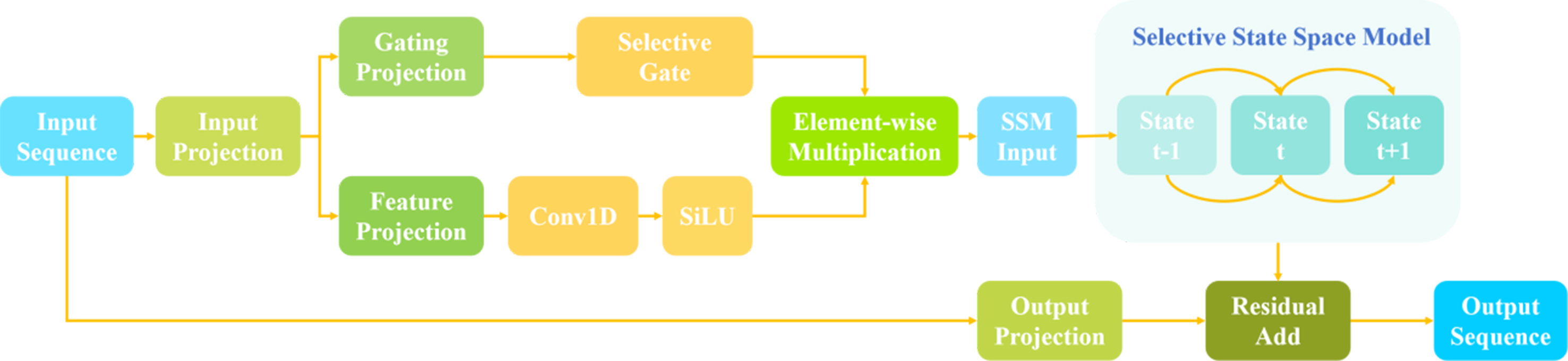
Figure 3. Structure of the Mamba state-space modeling module. SSM: State space models.
In this study, Mamba is employed to efficiently model the full life-cycle capacity curve of lithium-ion batteries. The degradation process exhibits strong long-term dependencies, and relying solely on local statistical features fails to represent the overall degradation trend. The SSM mechanism in Mamba dynamically updates hidden states through parameterized transition matrices (A, B, C, Δ, D), capturing both short-term fluctuations and long-term decay patterns. This enables the model to generate stable feature representations for RUL prediction.
The Mamba module consists of four components:
Input projection (in_proj) - The input sequence is linearly mapped into two parts: a hidden-state representation and a residual signal. This prepares the data for state updates and subsequent feature fusion.
Depthwise convolution (conv1d) - A one-dimensional depthwise convolution is applied along the sequence dimension to extract local neighborhood information and enhance temporal smoothness. This operation is implemented as grouped convolution in the MambaBlock.
State-space recurrence (ssm) - The module performs the Selective Scan process using parameterized matrices A, B, C, D and a dynamic step size ∆ computed from the input, as expressed in Equation (5)[32].
In Equation (5), xt denotes the hidden state of the state-space model at time step t, and xt-1 is the previous hidden state. ut represents the input signal derived from the projected feature sequence, while yt denotes the output of the SSM at the current step. A, B, C, and D are learnable state transition, input mapping, output projection, and direct feed-through matrices, respectively, which jointly govern the evolution of the system dynamics. The term Δ acts as a data-dependent dynamic step size, modulating the discrete-time update and enabling the selective scan mechanism to adjust temporal scaling adaptively. Here, ∆ is constrained to be non-negative through the softplus function, ensuring reasonable time-step scaling. This mechanism is the key for Mamba to effectively capture long-range dependencies.
Residual connection and output projection (out_proj) - The recursive output is combined with the residual signal and projected linearly back to the original dimension. This preserves information and enhances representational capacity.
In the overall framework, the hidden-state sequence output by the Mamba module is used to generate contextual representations and is further combined with the trend-constrained module (MDH) to ensure physically consistent predictions.
2.4. MDH
In lithium-ion battery lifetime prediction, battery capacity generally follows an overall decreasing trend as the cycle number increases. However, apparent local recovery may occur because of relaxation effects, temperature variations, or measurement noise. Purely data-driven deep learning models may violate this degradation characteristic and generate locally increasing predictions that lack physical plausibility and interpretability. To address this, a MDH is designed to impose a physical constraint on the predicted capacity at the output stage, as shown in Figure 4.
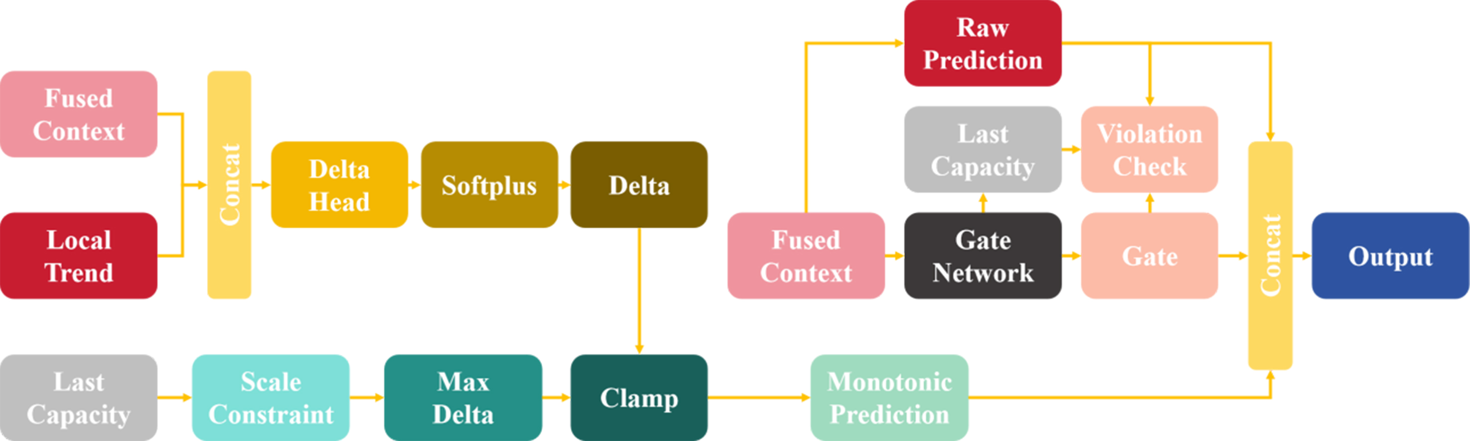
Figure 4. Structure of the MDH module. MDH: Monotonic decreasing head.
To ensure non-increasing capacity, the MDH outputs a non-negative “decrement value” and constrains its relative magnitude. The result is then adaptively fused with the original regression head through a gating mechanism. The previous-step capacity yt, local trend Δht = htlast - ht-1last, and contextual representation ct are all integrated in this process.
The trend-aware decrement is defined in Equation (6).
In Equation (6), ct denotes the contextual hidden representation output by the sequence encoder at step t, while Δht represents the local trend descriptor extracted from the recent degradation trajectory. The function fθ(·) is a two-layer multilayer perceptron that maps the concatenated features into a latent decrement score, which is then transformed into a non-negative value through the softplus function. The upper bound of the relative decrement is defined in Equation (7).
This structure ensures that the predicted capacity strictly decreases across cycles. The monotonic branch is expressed in Equation (8).
In Equation (8), yt+1mono denotes the monotonicity-enforced capacity prediction. The term yt is the previous capacity. The fusion of the main and auxiliary prediction branches is defined in Equation (9).
In Equation (9),
In Equation (10), gt is a gating coefficient that adaptively increases when a physical violation occurs, directing the prediction toward the monotonic branch. The term Wg is the learnable projection matrix that maps the contextual representation ct into a gating score, while β amplifies the gate when the intermediate prediction yt+1mono exceeds the previous value yt. The indicator function [
The MDH module integrates three types of inputs: the contextual representation at the current step, local trend information, and the previous capacity value. It outputs the predicted capacity change Δ, which is strictly non-negative. A relative upper bound constraint is applied to Δ, ensuring that the decrease does not exceed a certain ratio of the previous capacity. The final predicted capacity is then obtained by
Additionally, the MDH is fused with the main prediction branch (original regression head) through an adaptive gating mechanism. When the main prediction violates physical constraints (i.e., the predicted capacity exceeds the previous value), the gate value increases, assigning higher weight to the physically consistent branch. When the prediction follows the physical rule, the main branch dominates. This adaptive fusion achieves a balance between physical consistency and model flexibility.
Practical note. In real-world battery operation, apparent local capacity recovery can be observed due to relaxation phenomena, temperature changes, and measurement noise. The proposed MDH is intended to improve long-horizon trend consistency and suppress non-physical upward oscillations in predictions, rather than to explicitly model reversible short-term behaviors. Therefore, strict monotonic enforcement may reduce flexibility in scenarios dominated by recovery effects, particularly in early-life stages. Exploring soft/uncertainty-aware monotonic constraints is an important direction for future work.
3. EXPERIMENTS
3.1. Dataset
This study uses the National Aeronautics and Space Administration (NASA) battery dataset as the primary benchmark and introduces the TJU dataset to evaluate the generalization capability of the proposed model under multivariable conditions[32]. The NASA dataset, provided by the NASA, contains full discharge cycle data for four lithium-ion batteries (B0005, B0006, B0007, and B0018) under constant operating conditions. The core variable is the trajectory of capacity degradation with respect to cycle count, which has become one of the most widely used benchmark datasets for RUL prediction. To simulate practical rolling prediction scenarios, the capacity sequences were truncated at different starting points (SP = 50, 70, and 90) to initialize the prediction process. These settings cover both the early and rapid degradation stages, enabling evaluation of model stability and robustness under different observation windows.
In contrast, the TJU dataset, proposed by Tongji University and collaborators, provides more complex cycling information. In addition to capacity, it includes multiple statistical features of voltage and current during constant current (CC) and constant voltage (CV) stages, such as mean, variance, kurtosis, skewness, slope, and entropy. Incorporating the TJU dataset serves two purposes: Firstly, to demonstrate that the proposed model maintains strong predictive performance in high-dimensional feature spaces; and secondly, to verify its generalization capability across datasets. For consistency, the TJU dataset was evaluated at starting points SP is equal to 200, 300, and 400, allowing assessment of prediction behavior over longer historical cycles.
Notably, although the NASA dataset is essentially univariate, the input sequence is first projected into a higher-dimensional latent space before being processed by CGHF. Therefore, multi-scale feature extraction is still performed across latent channels. Nevertheless, the full advantage of CGHF is more evident in multivariate scenarios, which is further validated using the TJU dataset.
Figure 5 illustrates the capacity degradation curves of the two datasets, while Table 1 lists the basic specifications of the cells, including model type, rated capacity, charge–discharge protocol, and temperature conditions.
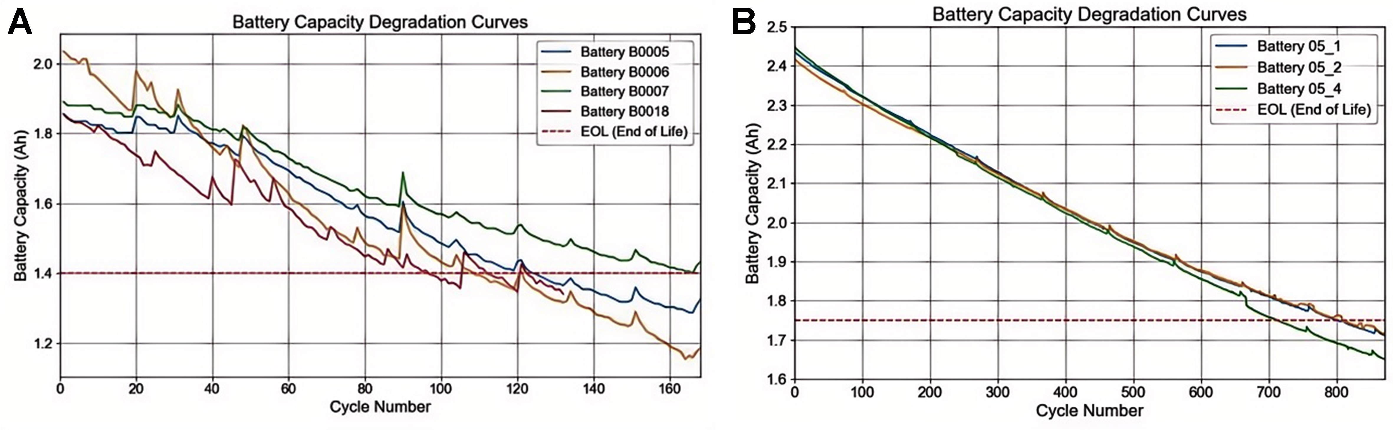
Figure 5. (A) NASA dataset and (B) TJU dataset: capacity degradation curves of lithium-ion batteries in both datasets. NASA: National Aeronautics and Space Administration; TJU: Tongji University.
Battery parameter information of the NASA and TJU datasets
| Source | ID | Charge/discharge cut-off voltage | Charge/discharge CC | Temperature | Rated capacity | End-of-Life criteria |
| NASA | B0005 | 4.2 V / 2.7 V | 1.5 A / 2 A | 24 °C | 2 Ah | 1.4 Ah |
| B0006 | 4.2 V / 2.5 V | 1.5 A / 2 A | 24 °C | 2 Ah | 1.4 Ah | |
| B0007 | 4.2 V / 2.2 V | 1.5 A / 2 A | 24 °C | 2 Ah | 1.4 Ah | |
| B0018 | 4.2 V / 2.5 V | 1.5 A / 2 A | 24 °C | 2 Ah | 1.4 Ah | |
| TJU | CY25_1 | 4.2 V / 2.5 V | 1.25 A / 2.5 A | 25 °C | 2.5 Ah | 1.75 Ah |
| CY25_2 | 4.2 V / 2.5 V | 1.25 A / 2.5 A | 25 °C | 2.5 Ah | 1.75 Ah | |
| CY25_4 | 4.2 V / 2.5 V | 1.25 A / 2.5 A | 25 °C | 2.5 Ah | 1.75 Ah |
3.2. Data cleaning and feature construction
For the NASA dataset, the raw records contain missing cycles and local abnormal fluctuations; therefore, a two-step correction strategy is adopted. Initially, the entire cycle range from 1 to the maximum is completed, and missing capacity values are reconstructed by linear interpolation. Subsequently, outliers are detected using the 2σ criterion and masked, followed by another linear interpolation to smooth the capacity trajectory. The resulting capacity curve becomes smoother and exhibits an approximately monotonic decline, which is consistent with the overall irreversible degradation trend of lithium-ion batteries under controlled cycling.
Notably, the above interpolation and sigma-based masking are mainly used to handle missing cycles and apparent outliers in the NASA records, rather than to remove realistic short-term recovery behaviors. This preprocessing results in a smoother and approximately monotonic trajectory, which may attenuate local capacity recovery caused by relaxation or measurement noise. Accordingly, the current benchmark setting may not fully reflect reversible short-term behaviors, and we regard evaluation on raw (non-monotonized) trajectories under broader operating conditions as an important direction for future work.
For the TJU dataset, the 3σ rule is applied to all numerical feature columns, removing rows where values exceed three standard deviations from the mean. The cycle indices are then renumbered to ensure sequence continuity. In the feature selection stage, 17 health-related statistical features are retained, including the mean, standard deviation, kurtosis, skewness, slope, and entropy of voltage and current during the CC and CV phases, as well as charging time and capacity. Compared with the univariate NASA dataset, the multidimensional TJU features provide a more comprehensive description of the degradation process, supporting verification of the model’s variable selection and channel attention mechanisms.
3.3. Data partitioning
As shown in Table 2, all data are divided into two parts: a training set and a test set. Within the training data, the first 80% of cycles in chronological order are used for model training, and the remaining 20% are used for validation to monitor early stopping and select hyperparameters. For the NASA dataset, which serves as the main experimental benchmark, the full-cycle data from batteries B0006, B0007, and B0018 are used for training, while B0005 is reserved as an independent test sample to evaluate cross-cell generalization and rolling prediction performance at different starting points (SP). For the TJU dataset, which tests generalization in a multivariable feature space, CY25_2 and CY25_4 are merged as the training set, and CY25_1 is used for testing.
Partitioning of the NASA and TJU datasets
| Dataset | Training dataset | Test dataset |
| NASA | B0006 B0007 B0018 | B0005 |
| TJU | CY25_2 CY25_4 | CY25_1 |
During testing, evaluation begins at the predefined starting points for each dataset (NASA: 50/70/90; TJU: 200/300/400). To strictly prevent data leakage, all normalization parameters are computed exclusively from the training set and then fixed for use in validation and testing. This setup ensures independence under cross-battery conditions and maintains consistency in constructing multi-start and single-step prediction windows, facilitating fair comparisons between datasets and reproducibility of experiments.
3.4. Overall architecture
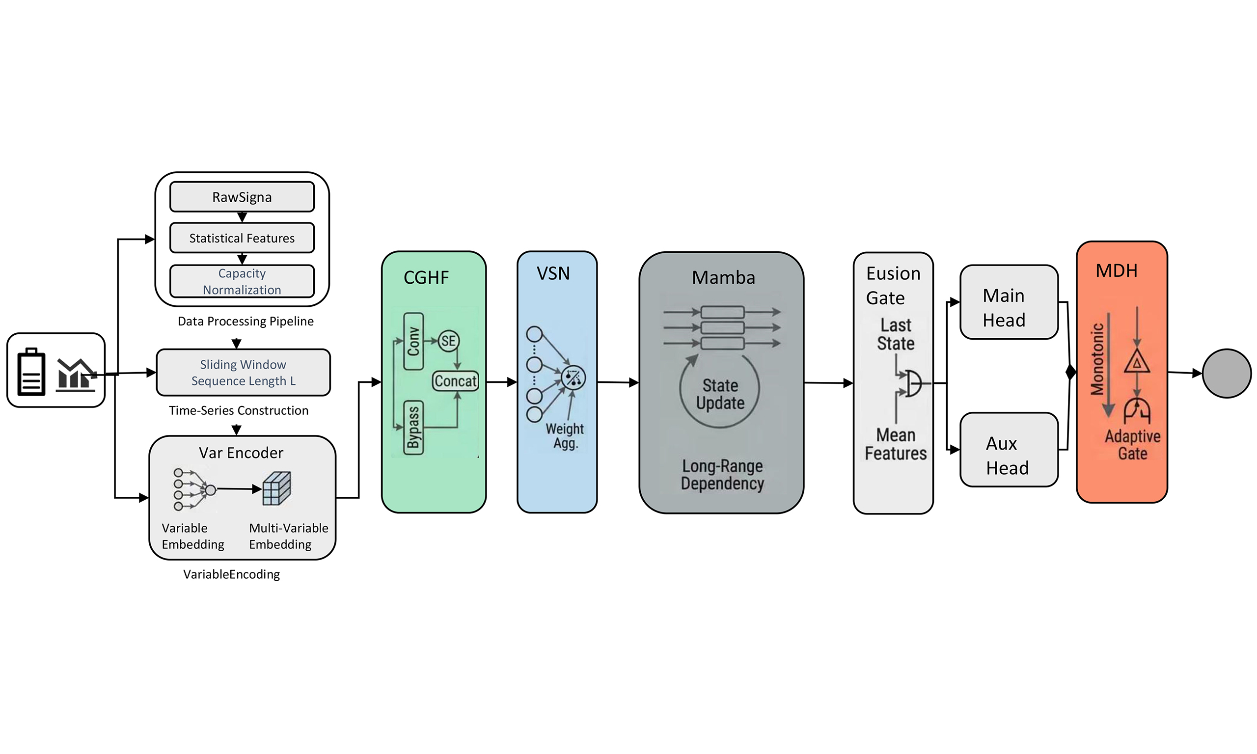
The model architecture consists of four main components, and the overall framework is shown in Figure 6.
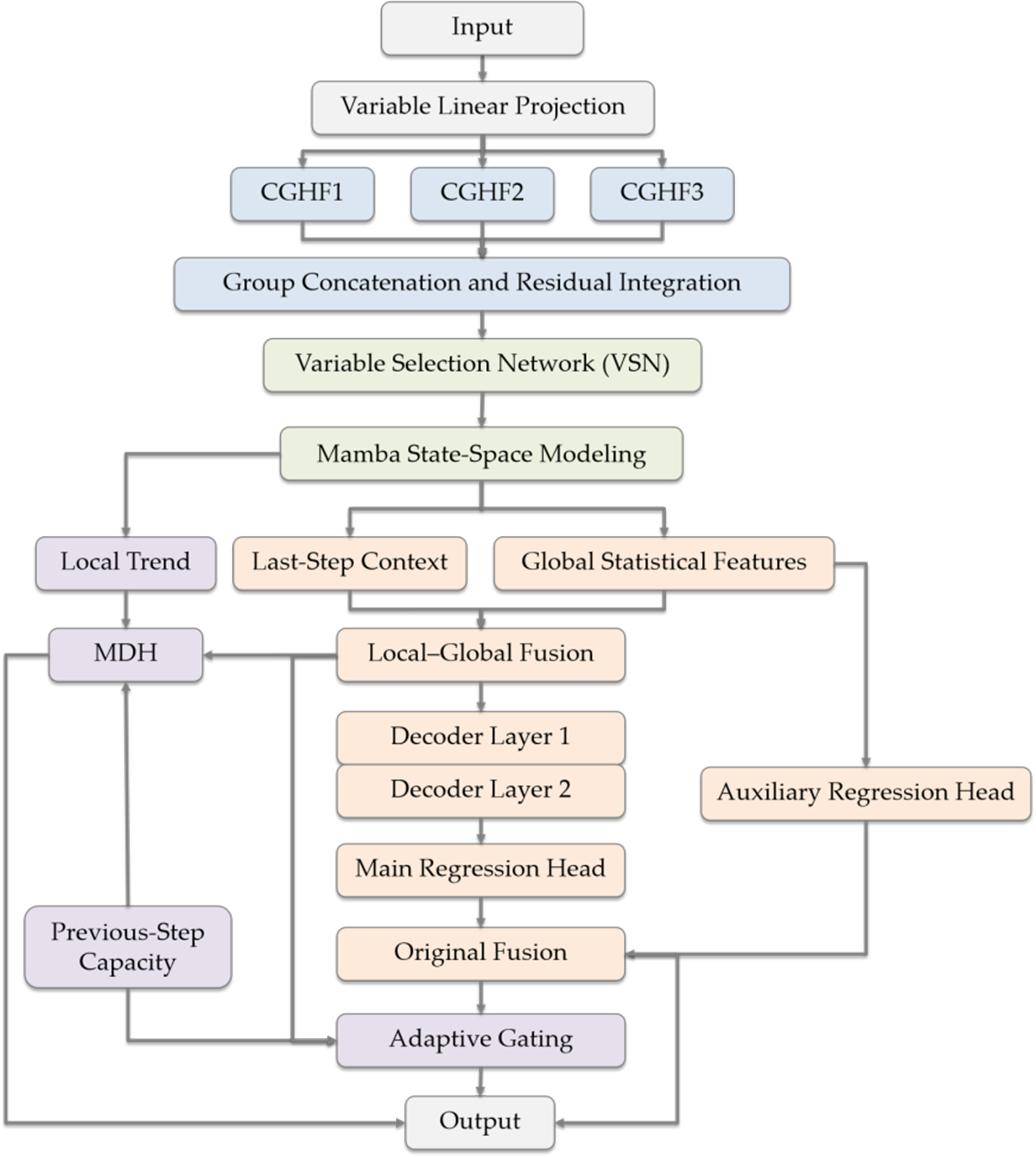
Figure 6. Overall architecture of the proposed CGHF-MDH-Mamba model. CGHF: Channel-grouping half-convolution; MDH: monotonic decreasing head.
First, CGHF operates at the channel level to compress redundant feature maps and enhance local temporal patterns with lightweight grouped half-convolution and channel attention before sequence modeling. Additionally, VSN operates at the variable level to assign adaptive importance weights across heterogeneous input variables, improving feature saliency and interpretability in multivariate settings. In this sense, CGHF and VSN play complementary roles: the former suppresses intra-channel redundancy, while the latter reduces inter-variable redundancy. Third, the Mamba sequence modeling module captures long-range dependencies and fuses local and global contextual information to better represent complex degradation patterns after feature refinement. Finally, a MDH imposes a physical constraint that forces the predicted capacity to decrease monotonically with cycles, ensuring consistency with electrochemical degradation laws. These modules operate in a complementary manner to improve multivariate degradation modeling, prediction consistency, and generalization capability.
4. RESULTS AND DISCUSSION
4.1. Experimental environment
The experiments were conducted on an Ubuntu 22.04 operating system using the PyTorch deep learning framework. The detailed hardware and software configurations are listed in Table 3.
Experimental environment configuration
| Item | Configuration information |
| Operating system | Ubuntu 22.04 |
| Development language | Python 3.10.13 |
| Framework | PyTorch 1.13.1 + cuda 11.7 |
| CPU | Intel(R) Core(TM) i5-14600KF |
| GPU | GeForce RTX 4070 Ti SUPER(16G) |
| Memory | 64 GB |
During training, the AdamW optimizer was used with a learning rate of 1 × 10⁻³, a batch size of 128, and a maximum of 1,000 epochs. An early stopping strategy was applied to prevent overfitting. The sequence length was set to 64, and the prediction step was set to 1. All hyperparameters were tuned based on validation performance to ensure fairness and reproducibility of the experimental results.
4.2. Evaluation metrics
In this study, five evaluation metrics are used to assess the prediction performance of the model at each starting point (SP): mean absolute error (MAE), root mean square error (RMSE), coefficient of determination (R2), absolute error (AE), and relative error (RE). The definitions and corresponding formulas for these metrics are summarized in Table 4. In this study, MAE and RMSE are calculated on battery capacity prediction values and are reported in Ah. AE is reported in cycles, whereas R2 and RE are dimensionless.
Evaluation indicators
| Evaluation metrics | Formula | Significance |
| MAE (Ah) | The absolute value of the error between the predicted and true values is averaged. Value range: ≥ 0, the smaller the better | |
| RMSE (Ah) | Similar to MAE, but more sensitive to “points with large deviations”. Value range: ≥ 0, the smaller the better | |
| R2 | Measures the degree to which predicted values explain true values. Numerical range: (-∞; 1], the closer the perfect prediction is to 1, the better | |
| AE (for RUL, cycles) | The difference between the predicted RUL (remaining life cycle number) and the real RUL | |
| RE (for RUL) | The ratio of RUL prediction error to true life. Value range: 0-1, the smaller the better |
4.3. Comparative experiments
To comprehensively evaluate the performance of the proposed model, comparative experiments were conducted on both the NASA and TJU battery datasets.
For the NASA dataset, which primarily consists of univariate sequences describing capacity degradation over cycles, the experiments focused on evaluating the model’s RUL prediction capability based on a single health indicator. As shown in Figure 7 and Table 5, other deep learning models-such as Autoformer, FEDformer, and PatchTST-can partially capture the degradation trend but exhibit larger errors across different starting points (SP = 50, 70, and 90). In contrast, the RUL-Mamba model achieves lower prediction errors, benefiting from the ability of the state-space recurrence mechanism to model long-term dependencies. The proposed CGHF-MDH-Mamba model further improves prediction accuracy, achieving a minimum MAE of 0.0081. These results indicate that the integration of channel half-convolution and monotonic constraints improves prediction stability and maintains competitive performance in univariate scenarios.
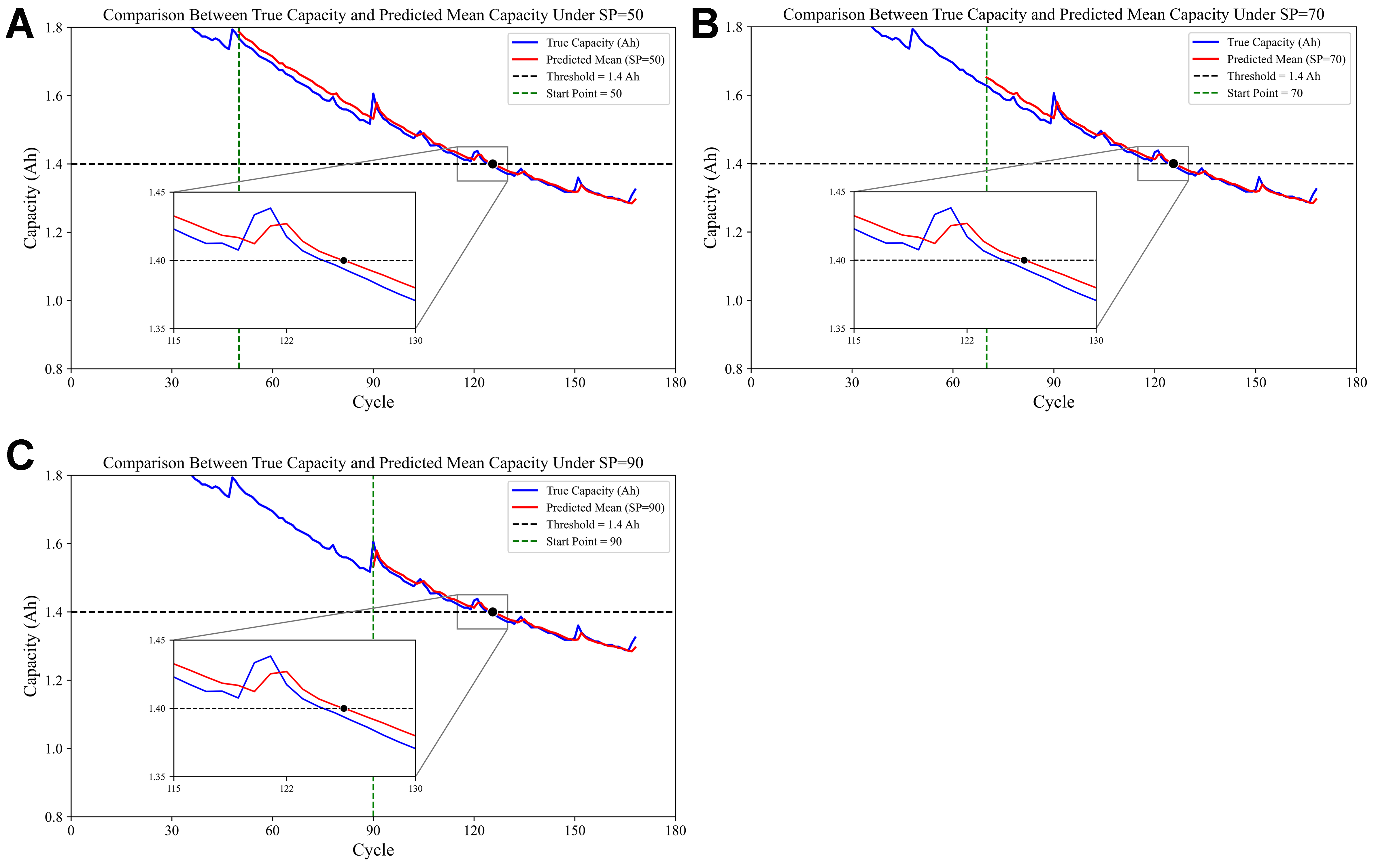
Figure 7. Comparison between predicted and measured battery capacity trajectories on the NASA dataset under different prediction starting points. Comparison curve between predicted value and true value when (A) SP = 50; (B) SP = 70; (C) SP = 90. NASA: National Aeronautics and Space Administration; SP: starting point.
RUL prediction results of different models on NASA dataset
| Dataset | Method | SP | TRUL | PRUL | MAE (Ah) | RMSE (Ah) | R2 | AE (cycles) | RE |
| NASA | Autoformer | 50 | 75 | 74.8 | 0.0234 | 0.0336 | 0.9341 | 3.6 | 0.0486 |
| 70 | 55 | 52.3 | 0.0230 | 0.0340 | 0.8721 | 4.1 | 0.0759 | ||
| 90 | 35 | 32.8 | 0.0213 | 0.0313 | 0.8153 | 4.2 | 0.1235 | ||
| FEDformer | 50 | 75 | 74.9 | 0.0215 | 0.0266 | 0.9569 | 4.7 | 0.0635 | |
| 70 | 55 | 53.6 | 0.0199 | 0.0262 | 0.9217 | 5.0 | 0.0926 | ||
| 90 | 35 | 32.6 | 0.0172 | 0.0237 | 0.8961 | 5.8 | 0.1706 | ||
| PathFormer | 50 | 75 | 70.3 | 0.0274 | 0.0375 | 0.9228 | 5.1 | 0.0689 | |
| 70 | 55 | 50.0 | 0.0214 | 0.0292 | 0.9100 | 5.6 | 0.1037 | ||
| 90 | 35 | 27.1 | 0.0186 | 0.0248 | 0.8941 | 7.9 | 0.2324 | ||
| TimesNet | 50 | 75 | 78.0 | 0.0364 | 0.0478 | 0.8753 | 3.0 | 0.0405 | |
| 70 | 55 | 57.9 | 0.0298 | 0.0403 | 0.8349 | 2.9 | 0.0537 | ||
| 90 | 35 | 38.0 | 0.0213 | 0.0275 | 0.8699 | 3.0 | 0.0882 | ||
| TimeMixer | 50 | 75 | 79.8 | 0.0239 | 0.0285 | 0.9540 | 8.0 | 0.1081 | |
| 70 | 55 | 52.7 | 0.0241 | 0.0298 | 0.9014 | 6.7 | 0.1241 | ||
| 90 | 35 | 26.0 | 0.0203 | 0.0307 | 0.8290 | 9.0 | 0.2647 | ||
| PatchTST | 50 | 75 | 79.2 | 0.0260 | 0.0319 | 0.9405 | 4.2 | 0.0568 | |
| 70 | 55 | 56.7 | 0.0201 | 0.0250 | 0.9333 | 3.9 | 0.0722 | ||
| 90 | 35 | 30.4 | 0.0150 | 0.0212 | 0.9209 | 5.0 | 0.1471 | ||
| MambaLithium | 50 | 75 | 81.7 | 0.0301 | 0.0362 | 0.9254 | 6.7 | 0.0905 | |
| 70 | 55 | 60.7 | 0.0250 | 0.0305 | 0.9034 | 5.7 | 0.1056 | ||
| 90 | 35 | 32.9 | 0.0188 | 0.0244 | 0.8943 | 4.1 | 0.1206 | ||
| RUL-Mamba | 50 | 75 | 75.8 | 0.0083 | 0.0134 | 0.9901 | 0.8 | 0.0135 | |
| 70 | 55 | 55.9 | 0.0091 | 0.0150 | 0.9770 | 0.9 | 0.0167 | ||
| 90 | 35 | 34.5 | 0.0092 | 0.0161 | 0.9556 | 2.5 | 0.0735 | ||
| Ours | 50 | 75 | 76 | 0.0081 | 0.0132 | 0.9848 | 1.0 | 0.0133 | |
| 70 | 55 | 56 | 0.0082 | 0.0135 | 0.9816 | 1.0 | 0.0182 | ||
| 90 | 35 | 36 | 0.0085 | 0.0144 | 0.9640 | 1.0 | 0.0286 |
For the TJU dataset, which includes multivariate health indicators such as voltage and current statistics across different charge–discharge phases, the experiments focused on evaluating multivariate time-series prediction performance. As shown in Figure 8 and Table 6, conventional Transformer-based models achieved relatively good fitting performance but still suffered from inconsistencies and higher errors across starting points. In contrast, the RUL-Mamba model effectively exploited temporal dependencies among variables, producing very low prediction errors. Building on this, the proposed CGHF-MDH-Mamba model achieved further improvement, reducing the MAE to 0.0009 and yielding an RUL deviation of only one cycle from the ground truth. These results indicate that, in complex multivariate conditions, the CGHF’s redundant feature compression and MDH’s trend constraint mechanisms significantly enhance generalization capability.
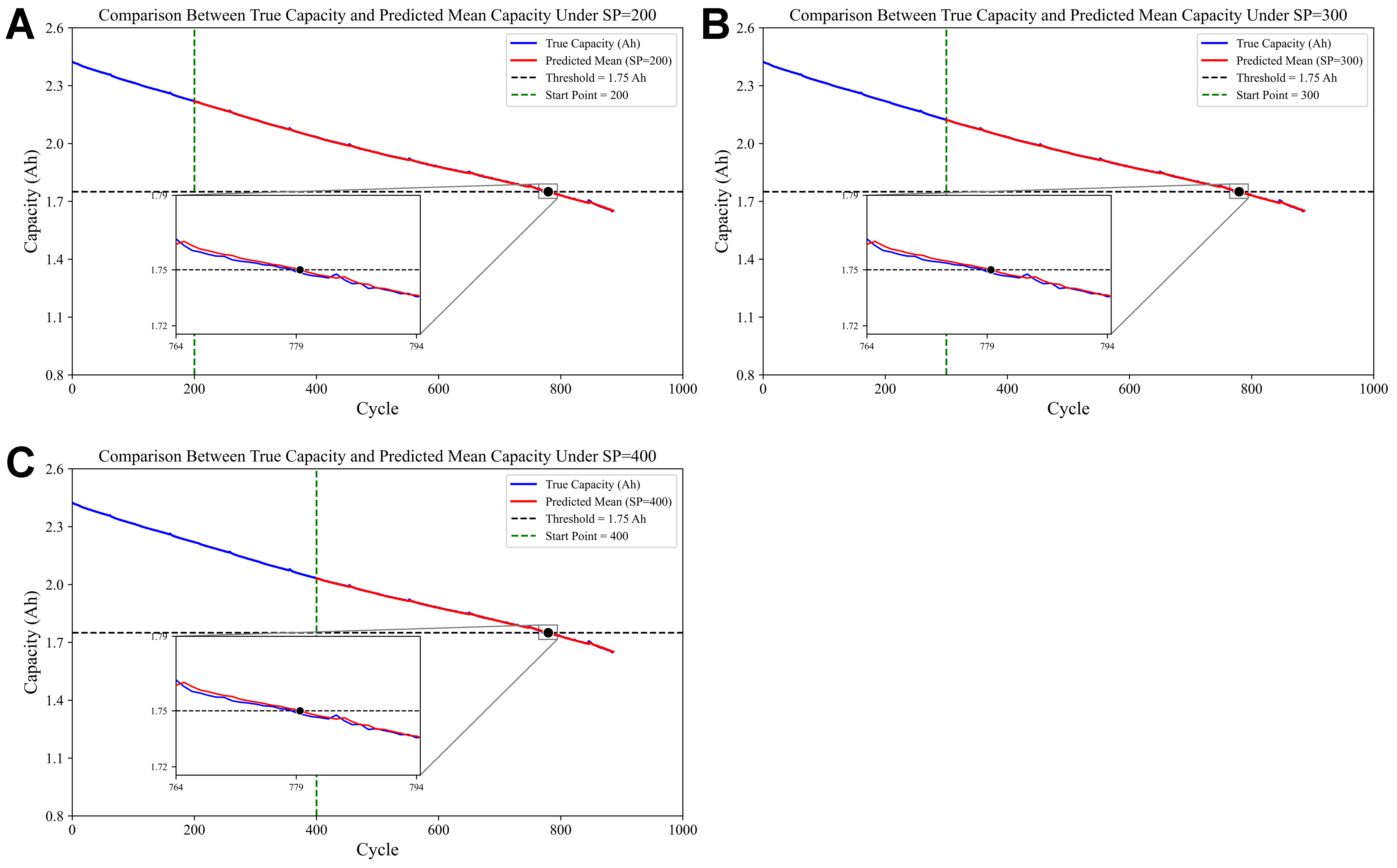
Figure 8. Comparison between predicted and measured battery capacity trajectories on the TJU dataset under different prediction starting points. Comparison curve between predicted value and true value when (A) SP = 200; (B) SP = 300; (C) SP = 400. TJU: Tongji University; SP: starting point.
RUL prediction results of different models with multivariate inputs on TJU dataset
| Dataset | Method | SP | TRUL | PRUL | MAE (Ah) | RMSE (Ah) | R2 | AE (cycles) | RE |
| TJU | Autoformer | 200 | 579 | 580.4 | 0.0020 | 0.0028 | 0.9997 | 1.6 | 0.0028 |
| 300 | 479 | 478.6 | 0.0031 | 0.0042 | 0.9989 | 3.2 | 0.0067 | ||
| 400 | 379 | 376.6 | 0.0038 | 0.0051 | 0.9975 | 4.4 | 0.0116 | ||
| FEDformer | 200 | 579 | 581.2 | 0.0020 | 0.0028 | 0.9997 | 2.2 | 0.0038 | |
| 300 | 479 | 481.5 | 0.0030 | 0.0039 | 0.9990 | 2.5 | 0.0052 | ||
| 400 | 379 | 380.2 | 0.0034 | 0.0045 | 0.9980 | 3.2 | 0.0085 | ||
| PathFormer | 200 | 579 | 569.2 | 0.0093 | 0.0123 | 0.9938 | 9.8 | 0.0170 | |
| 300 | 479 | 467.4 | 0.0105 | 0.0148 | 0.9868 | 11.6 | 0.0243 | ||
| 400 | 379 | 364.4 | 0.0144 | 0.0199 | 0.9641 | 14.6 | 0.0386 | ||
| TimesNet | 200 | 579 | 580.0 | 0.0161 | 0.0202 | 0.9832 | 1.0 | 0.0017 | |
| 300 | 479 | 479.1 | 0.0145 | 0.0177 | 0.9812 | 0.1 | 0.0002 | ||
| 400 | 379 | 378.3 | 0.0129 | 0.0154 | 0.9787 | 0.7 | 0.0019 | ||
| TimeMixer | 200 | 579 | 582.2 | 0.0120 | 0.0147 | 0.9900 | 12.0 | 0.0208 | |
| 300 | 479 | 456.3 | 0.0195 | 0.0236 | 0.9630 | 35.1 | 0.0734 | ||
| 400 | 379 | 334.4 | 0.0271 | 0.0308 | 0.8992 | 51.4 | 0.1360 | ||
| PatchTST | 200 | 579 | 574.8 | 0.0087 | 0.0113 | 0.9947 | 8.8 | 0.0152 | |
| 300 | 479 | 456.6 | 0.0206 | 0.0233 | 0.9640 | 22.8 | 0.0477 | ||
| 400 | 379 | 334.9 | 0.0326 | 0.0347 | 0.8740 | 44.1 | 0.1167 | ||
| MambaLithium | 200 | 579 | 580.9 | 0.0064 | 0.0082 | 0.9970 | 4.7 | 0.0081 | |
| 300 | 479 | 472.3 | 0.0088 | 0.0110 | 0.9919 | 6.7 | 0.0140 | ||
| 400 | 379 | 354.3 | 0.0178 | 0.0197 | 0.9631 | 24.7 | 0.0653 | ||
| RUL-Mamba | 200 | 579 | 581.6 | 0.0014 | 0.0022 | 0.9998 | 2.6 | 0.0045 | |
| 300 | 479 | 481.6 | 0.0015 | 0.0023 | 0.9997 | 2.6 | 0.0054 | ||
| 400 | 379 | 381.6 | 0.0016 | 0.0024 | 0.9995 | 2.6 | 0.0069 | ||
| Ours | 200 | 579 | 580.0 | 0.0009 | 0.0015 | 0.9999 | 1.0 | 0.0017 | |
| 300 | 479 | 480.0 | 0.0010 | 0.0016 | 0.9999 | 1.0 | 0.0021 | ||
| 400 | 379 | 380.0 | 0.0010 | 0.0016 | 0.9998 | 1.0 | 0.0026 |
Overall, the experimental results demonstrate that, for univariate input scenarios (NASA dataset), the RUL-Mamba model already exhibits strong prediction capability, while the proposed model further improves both prediction accuracy and physical consistency. For multivariate input scenarios (TJU dataset), the inclusion of CGHF and MDH modules significantly enhances the model’s ability to select and represent multidimensional degradation features, achieving the best performance across all starting points. These findings confirm that the CGHF-MDH-Mamba model maintains strong adaptability and generalization under various data characteristics and operating conditions.
4.4. Ablation study
To quantify the contribution of each module to the performance improvement of the proposed battery RUL prediction model, a systematic ablation study was conducted. The experiments were performed on the TJU dataset by progressively integrating different modules. Starting from the baseline model, the MDH, fusion, VSN, and CGHF modules were added one by one, and the final results were compared with the complete model. The detailed results are shown in Table 7.
Comparison of ablation experiment results
| Method | SP | MAE (Ah) | RMSE (Ah) | R2 | AE (cycles) | RE | Inference time/s |
| Base model | 200 | 0.0014 | 0.0022 | 0.9998 | 2.6 | 0.0045 | 0.203 |
| 300 | 0.0015 | 0.0023 | 0.9997 | 2.6 | 0.0054 | 0.152 | |
| 400 | 0.0016 | 0.0024 | 0.9995 | 2.6 | 0.0069 | 0.126 | |
| Base model + MDH | 200 | 0.0018 | 0.0021 | 0.9998 | 1.4 | 0.0024 | 0.171 |
| 300 | 0.0018 | 0.0022 | 0.9997 | 1.4 | 0.0029 | 0.128 | |
| 400 | 0.0018 | 0.0022 | 0.9995 | 1.4 | 0.0037 | 0.110 | |
| Base model + fusion + MDH | 200 | 0.0016 | 0.0020 | 0.9998 | 1.2 | 0.0021 | 0.166 |
| 300 | 0.0016 | 0.0020 | 0.9998 | 1.2 | 0.0025 | 0.127 | |
| 400 | 0.0016 | 0.0020 | 0.9996 | 1.2 | 0.0032 | 0.105 | |
| Base model + VSN + fusion + MDH | 200 | 0.0012 | 0.0016 | 0.9999 | 1.0 | 0.0017 | 0.177 |
| 300 | 0.0012 | 0.0017 | 0.9998 | 1.0 | 0.0021 | 0.129 | |
| 400 | 0.0012 | 0.0017 | 0.9997 | 1.0 | 0.0026 | 0.105 | |
| Base model + CGHF + VSN + fusion + MDH | 200 | 0.0009 | 0.0015 | 0.9999 | 1.0 | 0.0017 | 0.167 |
| 300 | 0.0010 | 0.0016 | 0.9999 | 1.0 | 0.0021 | 0.119 | |
| 400 | 0.0010 | 0.0016 | 0.9998 | 1.0 | 0.0026 | 0.102 |
As observed from the results, the baseline model already achieved reasonably stable prediction performance in terms of MAE and RMSE, but the AE in RUL estimation remained relatively high. After introducing the MDH module, MAE and RMSE improved slightly, while AE dropped significantly. This indicates that MDH enhances the consistency between predicted and actual RUL values and enforces the physical law of monotonic capacity degradation.
When the fusion gating mechanism was added on top of the Baseline + MDH structure, the model combined local and global contextual representations, improving the smoothness and stability of the predicted curves. The approach reduces fluctuations caused by overreliance on instantaneous features. On this basis, incorporating the VSN module led to a more substantial improvement-MAE dropped to 0.0012. This demonstrates that the VSN effectively suppresses noisy features and emphasizes key signals sensitive to degradation trends, thereby enhancing both prediction accuracy and interpretability in multivariable input scenarios.
Overall, after adding the CGHF module, the model achieved the best performance across all three starting points, with the lowest MAE reaching 0.0009, RMSE remaining around 0.0015, and AE controlled within one cycle. The CGHF module balances local feature extraction and channel residual connection through grouped half-convolution. Assisted by SE attention, it strengthens the response to key channels, making the overall feature representation more compact and effective. Together with the VSN’s sparse variable selection, this ensures strong robustness under high-dimensional feature conditions.
Moreover, inference efficiency was compared in the ablation experiments. It was found that even after adding multiple modules, the increase in inference time remained within a controllable range. The complete model maintained inference latency between 0.1 and 0.2 s. This demonstrates that the proposed approach achieves high prediction accuracy without significantly compromising computational efficiency, indicating potential suitability for online monitoring scenarios, subject to further validation under diverse operating conditions.
Collectively, the ablation results confirm that MDH is indispensable for maintaining physical consistency. The fusion and VSN modules enhance the expressiveness and robustness of temporal features, while CGHF further optimizes local modeling and channel feature selection. These components complement each other, enabling the complete CGHF-MDH-Mamba model to achieve an optimal balance among prediction accuracy, physical interpretability, and inference efficiency.
5. CONCLUSIONS
This paper proposes a unified framework for lithium-ion battery lifetime prediction that integrates CGHF, VSN, Mamba state-space modeling, and a MDH. Experimental results on the NASA and TJU datasets show that the proposed method provides competitive prediction accuracy while maintaining physical consistency and interpretability, summarized in three aspects as follows:
(1) Feature modeling: The CGHF and VSN modules contribute to local temporal feature extraction and multivariable sparse selection, respectively, effectively reducing redundancy and emphasizing critical features.
(2) Sequence modeling: The Mamba module efficiently captures long-range dependencies through a state-space recurrence mechanism, improving the model’s ability to represent full-lifecycle degradation trends.
(3) Prediction constraint: The MDH module introduces a monotonic decreasing constraint and an adaptive gating mechanism at the output stage, ensuring that the predictions follow electrochemical principles and reducing the deviation between predicted and actual RUL values.
Nevertheless, this work has several limitations. The datasets used in this study are primarily collected under controlled laboratory conditions, lacking the variability of real-world operating environments such as fluctuating temperatures, dynamic loads, and measurement noise. Although cross-dataset validation partially demonstrates generalization, further evaluation under diverse industrial conditions is necessary. In addition, while the proposed MDH introduces physical constraints that improve robustness, its effectiveness under extreme or highly non-stationary conditions requires further investigation. Future work will focus on large-scale real-world datasets and adaptive modeling strategies for complex operating scenarios.
DECLARATIONS
Authors’ contributions
Writing - original draft, software, investigation, methodology, validation, data curation: Zhou, X.
Supervision, conceptualization, writing - review and editing, resources, project administration, funding acquisition: Li, Y.
Investigation, methodology, visualization: Han, W.
Formal analysis, software, validation: Zhong, F.
Data curation, formal analysis, writing - review and editing: Zhang, Z.
Validation, visualization, resources: Tong, R.
Conceptualization, methodology, supervision, writing - review and editing: Huang, L.
All authors have read and agreed to the published version of the manuscript.
Availability of data and materials
The original contributions presented in this study are included in the article. Further inquiries can be directed to the corresponding author.
AI and AI-assisted tools statement
Not applicable.
Financial support and sponsorship
This research was funded by The Science and Technology Project of Southern Power Grid Company, Research on the Key Technology of Highly Refreshed Digital Twins and Large Depth Cable Detection in Power Conduit Corridors-Subject 1: Research on Key Technology of Highly Refreshed Digital Twins in Power Conduit Corridors (No. 030117KC23110003).
Conflicts of interest
Huang, L. serves as an Editorial Board Member of the journal Intelligence & Robotics. He was not involved in any steps of editorial processing, notably including reviewers’ selection, manuscript handling, or decision making. Li, Y.; Zhou, X.; Zhong, F.; Han, W.; Zhang, Z.; and Tong, R. are affiliated with Guangzhou Power Supply Bureau of Guangdong Power Grid Co., Ltd.
Ethical approval and consent to participate
Not applicable.
Consent for publication
Not applicable.
Copyright
© The Author(s) 2026.
REFERENCES
1. Sun, H.; Jiang, H.; Gu, Z.; et al. A novel multiple kernel extreme learning machine model for remaining useful life prediction of lithium-ion batteries. J. Power. Sources. 2024, 613, 234912.
2. Wang, S.; Li, Y. T.; Chen, L. F.; Su, X. H.; Zhou, S. B. Remaining useful life prediction of lithium-ion batteries based on IMM-PFF. Acta. Electron. Sin. 2025, 53, 1520-32.
3. Madani, S. S.; Shabeer, Y.; Fowler, M.; et al. Artificial intelligence and digital twin technologies for intelligent lithium-ion battery management systems. Batteries 2025, 11, 298.
4. Jia, D.; Ren, Y.; Li, L.; Yun, P.; Xue, Y.; Mi, Y. Research on optimization of hybrid energy storage capacity using ensemble empirical mode ecomposition and fuzzy control. Acta. Energ. Sol. Sin. 2023, 44, 239-46.
5. Zhu, Z. W.; Miao, J. W.; Zhu, X. Y.; et al. Research progress in remaining useful life prediction of lithium-ion batteries based on machine learning. Energy. Storage. Sci. Technol. 2024, 13, 3134-49.
6. Li, Y.; Wang, J. F.; Mo, W. Q.; Zhang, X. L. A review of remaining useful life prediction for lithium-ion batteries based on data-driven method. J. Power. Supply. 2025, 23, 253-65.
7. Ahwiadi, M.; Wang, W. A smart evolving fuzzy predictor with customized firefly optimization for battery RUL prediction. Batteries 2025, 11, 362.
8. Demirci, O.; Taskin, S.; Schaltz, E.; Acar Demirci, B. Review of battery state estimation methods for electric vehicles-Part II: SOH estimation. J. Energy. Storage. 2024, 96, 112703.
9. Liu, Y.; Tian, Y.; Liu, D.; et al. A novel dual gated recurrent unit neural network based on error compensation integrated with Kalman filter for the state of charge estimation of parallel battery modules. J. Power. Sources. 2025, 635, 236508.
10. Liu, B.; Yin, J.; Li, R. Improved particle filter algorithm for remaining useful life prediction of lithium-ion batteries. Power. Syst. Prot. Control. 2024, 52, 124-31.
11. Qiang, H.; Zhang, W.; Ding, K. A prediction framework for state of health of lithium-ion batteries based on improved support vector regression. J. Electrochem. Soc. 2023, 170, 110517.
12. Qaadan, S.; Alshare, A.; Popp, A.; Schmuelling, B. Prediction of lithium-ion battery health using GRU-BPP. Batteries 2024, 10, 399.
13. Zhao, S.; Sun, D.; Liu, Y.; Liang, Y. Remaining useful life prediction for lithium-ion batteries based on hybrid ensembles allied with data-driven approach. Energies 2025, 18, 1114.
14. Qian, K.; Li, Y.; Zou, Q.; Cao, K.; Li, Z. SOH and RUL estimation for lithium-ion batteries based on partial charging curve features. Energies 2025, 18, 3248.
15. Wang, X. M.; He, Y.; Wang, L. L.; Wu, H. B.; Xu, B.; Zhao, W. G. RUL prediction for lithium-ion batteries based on DWD-SVR model. Acta. Energ. Sol. Sin. 2025, 46, 52-9.
16. Cai, Y.; Wang, X.; Jiang, K.; Han, D.; Zhao, Q. Multi-step prediction of online lithium battery remaining useful life based on GRNN-GSA-ELM. J. Mech. Eng. 2024, 60, 296-308.
17. Zhang, T.; Sun, H. A method for predicting the remaining life of lithium-ion batteries based on an improved Dempster–Shafer evidence theory framework. Energies 2025, 18, 3370.
18. Sun, J.; Zhai, Q. C. A novel remaining useful life prediction method based on fusion feature and OOA-BiGRU for lithium-ion batteries. Trans. China. Electrotech. Soc. 2025, 40, 2996-3012.
19. Lv, K.; Ma, Z.; Bao, C.; Liu, G. Indirect prediction of lithium-ion battery RUL based on CEEMDAN and CNN-BiGRU. Energies 2024, 17, 1704.
20. Niu, W.; Li, X.; Tian, H.; Liang, C. Remaining useful life prediction of PEMFC based on 2-layer bidirectional LSTM network. World. Electr. Veh. J. 2025, 16, 511.
21. Liu, B.; Ji, C. L.; Cao, L. J.; Wu, X. Y.; Duan, Y. F. Prediction of remaining service life of lithium-ion batteries based on complete ensemble empirical mode decomposition with adaptive noise and BiLSTM-Transformer. Power. Syst. Prot. Control. 2024, 52, 167-77.
22. Mou, J.; Yang, Q.; Tang, Y.; Liu, Y.; Li, J.; Yu, C. Prediction of the remaining useful life of lithium-ion batteries based on the 1D CNN-BLSTM neural network. Batteries 2024, 10, 152.
23. Wang, X.; Zhang, J. Lithium battery lifespan prediction method integrating dynamic convolution transformer and CMA-ES. Acta. Energ. Sol. Sin. 2025, 46, 1-8.
24. Sun, Y.; An, J.; Huang, C.; et al. Battery life evaluation method based on temporal convolution network. Adv. Eng. Sci. 2025, 57, 259-68.
25. Yin, J.; Liu, B.; Sun, G.; Qian, X. Transfer learning DAE-LSTM for remaining useful life prediction of Li-ion batteries. Trans. China. Electrotech. Soc. 2024, 39, 290-302.
26. Saleem, U.; Liu, W.; Riaz, S.; et al. TransRUL: a transformer-based multihead attention model for enhanced prediction of battery remaining useful life. Energies 2024, 17, 3976.
27. Capoglu, E. U.; Taherkhani, A. A comparison of different transformer models for time series prediction. Information 2025, 16, 878.
28. Zhu, X.; Li, L.; Wang, G.; Shi, N.; Li, Y.; Yang, X. A lithium-ion battery remaining useful life prediction method based on mode decomposition and informer-LSTM. Electronics 2025, 14, 3886.
29. Wang, Z.; Ma, Y.; Gao, J.; Chen, H. Remaining useful life prediction for solid-state lithium batteries based on spatial–temporal relations and neuronal ODE-assisted KAN. Reliab. Eng. Syst. Saf. 2025, 260, 111003.
30. Jiang, L.; Li, Z.; Hu, C.; Chen, J.; Huang, Q.; He, G. A robust adapted flexible parallel neural network architecture for early prediction of lithium battery lifespan. Energy 2024, 308, 132840.
31. Zhou, J.; Huang, W.; Li, Y.; Wang, Z. Life prediction of lithium battery based on particle filter and BP neural network. J. Phys. Conf. Ser. 2024, 2814, 012047.
32. Huang, J.; Liu, L.; Zhao, H.; Li, T.; Li, B. RUL-Mamba: Mamba-based remaining useful life prediction for lithium-ion batteries. J. Energy. Storage. 2025, 120, 116376.
33. Liu, C.; Min, W.; Song, J.; et al. Channel grouping vision transformer for lightweight fruit and vegetable recognition. Expert. Syst. Appl. 2025, 292, 128636.
34. Liang, Y.; Zhao, S. Early prediction of remaining useful life for lithium-ion batteries with the state space model. Energies 2024, 17, 6326.
35. Liao, Z.; Lv, D.; Hu, Q.; Zhang, X. Review on aging risk assessment and life prediction technology of lithium energy storage batteries. Energies 2024, 17, 3668.
Cite This Article
How to Cite
Download Citation
Export Citation File:
Type of Import
Tips on Downloading Citation
Citation Manager File Format
Type of Import
Direct Import: When the Direct Import option is selected (the default state), a dialogue box will give you the option to Save or Open the downloaded citation data. Choosing Open will either launch your citation manager or give you a choice of applications with which to use the metadata. The Save option saves the file locally for later use.
Indirect Import: When the Indirect Import option is selected, the metadata is displayed and may be copied and pasted as needed.
About This Article
Copyright

Data & Comments
Data
0


Comments
Comments must be written in English. Spam, offensive content, impersonation, and private information will not be permitted. If any comment is reported and identified as inappropriate content by OAE staff, the comment will be removed without notice. If you have any queries or need any help, please contact us at [email protected].