


Modeling and prediction of the ionosphere with deep learning: a review
 0
0 Abstract
The ionosphere plays a crucial role in the transmission and propagation of space signals. As a component of the upper atmosphere, it exhibits distinct spatio-temporal variations and is influenced by solar and geomagnetic activities. Accurately modeling and predicting the ionosphere remains a significant challenge. Recent advancements in deep learning techniques have provided valuable insights into these challenges, offering new approaches for spatio-temporal ionospheric modeling and prediction. By integrating multiple observations from both space-borne and ground-based stations, high-resolution digital models of the ionosphere can be constructed using convolutional and recurrent neural networks. This paper reviews the recent progress in ionospheric modeling and prediction using deep learning networks, discusses the advantages of deep learning models over traditional empirical models, and outlines future directions to address the remaining challenges in this field.
Keywords
1. INTRODUCTION
The ionosphere, a key component of the Earth’s upper atmosphere, is formed through the ionization of neutral atoms and molecules by solar ultraviolet (UV) and extreme ultraviolet (EUV) radiation, and particle precipitation[1]. The importance of ionospheric modeling is closely tied to the advancement of modern aerospace technology, as the ionosphere serves as a critical medium for radio wave propagation. When radio signals from space or satellites pass through the ionosphere, they undergo refraction due to changes in plasma density with altitude, resulting in signal propagation delays[2,3]. The ionospheric plasma density exhibits small-scale structures, some of which approach the Fresnel scale of the radio waves, leading to rapid phase and amplitude fluctuations. This phenomenon is known as ionospheric scintillation[4]. Moreover, the ionosphere is intricately coupled with other regions of the near-Earth space environment, playing a vital role in space weather[5-7]. Specifically, the ionosphere can be influenced by extreme terrestrial weather events[8], tsunamis[9], explosions[10,11], rocket launches[12-14], and earthquakes[15-19].
Physics-based ionospheric modeling primarily relies on the principles of plasma physics, electromagnetics, and space fluid dynamics. It incorporates both physical and photochemical processes, particularly those related to the ionization of atmospheric molecules[20-22]. Several physics-driven ionospheric models have been developed and refined to solve the governing equations and elucidate the underlying mechanisms of ionospheric processes. These models allow for the calculation of the three-dimensional (3D), time-varying structures of neutral components, ion and electron densities, temperatures, and neutral winds within a predefined spatial range of the middle and upper atmosphere[23-25].
In addition, there are some empirical ionospheric models developed and increasingly adopted in both scientific research and engineering applications. These models largely reflect patterns observed in the ionosphere, capturing the combination of various physical processes[26-30]. Unlike physics-based models, empirical models rely on simple parameterizations and primarily focus on the F-region of the ionosphere. One well-known example is the international reference ionosphere (IRI), a global empirical model constructed using observational data from hundreds of ionospheric sounding stations and multiple satellite datasets[31]. Under specific solar activity conditions, the IRI model provides monthly averages of key ionospheric parameters, including electron density, critical frequency, electron and ion temperatures, and total electron content (TEC) across different regions. While it reproduces monthly climatological averages, the model shows deviations of up to 25% from actual measurements[31-33]. Despite its climatological nature, the IRI model remains a valuable tool for studying the spatiotemporal variations of the global ionosphere, based on observational data, and has facilitated the shift from physics-based to data-driven global ionospheric modeling approaches[34,35]. Another widely used empirical model is the NeQuick model, which describes the spatial distribution of electron density as a continuous function, ensuring the continuity of its first-order spatial derivative. This model extends beyond the F2 layer peak, encompassing both the bottom-side and topside ionosphere[36,37]. The ionospheric coverage in NeQuick is represented by a semi-Epstein layer, with its height determined by a thickness parameter. The model provides electron density and TEC along any path from Earth to a satellite and is widely recognized as the standard reference model for trans-ionospheric electromagnetic wave propagation. NeQuick is also used as the ionospheric single-frequency correction model for the GALILEO satellite navigation system[38-41].
The effects of radio wave propagation in the ionosphere enable the use of electromagnetic waves to sense variations in electron density and TEC. Radio wave propagation can be utilized to measure ionospheric electron density variations, while TEC is typically measured using dual-frequency Global Navigation Satellite Systems (GNSS) signals. In the early stages of ionospheric remote sensing, ionosondes and coherent/incoherent radar were the primary tools employed to uncover spatiotemporal patterns in the lower ionosphere[42]. Subsequently, dual-frequency GNSS observations provided an accurate method for measuring TEC along both slant and vertical paths. Space-borne radio occultation observations have further complemented 3D ionospheric modeling, offering novel insights into the fine-scale structure of the ionosphere[43]. Together, these observations form a large-scale spatiotemporal database for the ionosphere, laying the foundation for ionospheric modeling through artificial intelligence (AI)[44].
Modeling the ionosphere using AI relies on a vast array of multi-source data, including continuous and reliable ionospheric observations. Early data-driven studies of the ionosphere employed various machine learning (ML) techniques, such as decision trees, random forests, and eXtreme Gradient Boosting (XGBoost)[45-57]. These initial efforts laid a solid foundation for the application of more advanced and efficient neural network architectures in ionospheric research. With recent advances in AI, particularly deep learning (DL), the spatiotemporal morphology of the ionosphere can be more effectively investigated and understood, allowing for the detection and extraction of finer features. From a research perspective, the application of DL in ionospheric studies represents a shift from physics-based to data-driven approaches, marking a significant milestone in modern ionospheric research, as described by Figure 1. This trend reflects a broader transition from physics-inspired frameworks to data-driven paradigms, which heavily rely on neural network architectures and DL techniques. As part of AI for science, AI for space weather will play a pivotal role in future research, with DL remaining central to these advancements.
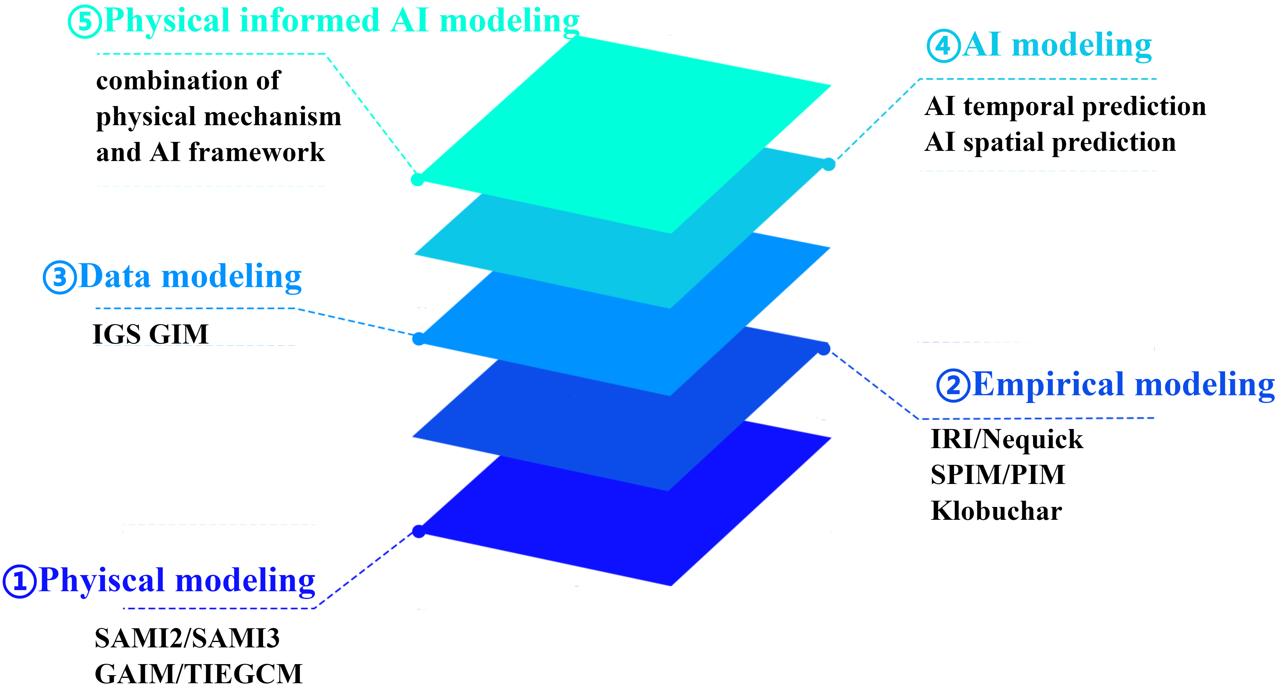
Figure 1. The research paradigms in ionosphere modeling. AI: Artificial intelligence; IGS: International GPS Service; GIM: Global Ionospheric Maps; IRI: international reference ionosphere; SPIM: Standard Plasmasphere Ionosphere Model; SAMI: Sami is Another Model of the Ionosphere; GAIM:Global Assimilative Ionosphere Model; TIEGCM: Thermosphere-Ionosphere-Electrodynamics General Circulation Mode.
2. IONOSPHERE AND ITS CURRENT OBSERVATIONS
The ionosphere consists of electrons, ions, and neutral particles in roughly equal proportions, with its properties determined by the balance between ionization, recombination, and transport processes. It is traditionally divided into distinct layers (D, E, F1, and F2) based on electron density profiles with altitude, each with characteristic formation mechanisms and behaviors. These layers exhibit different responses to solar and geomagnetic activity and play distinct roles in radio wave propagation[58].
The structure and variability of the ionosphere have profound implications for modern technological systems. High-frequency (HF) radio communications rely on ionospheric reflection for beyond-line-of-sight propagation, while GNSSs such as the United States’ Global Positioning System (GPS) and China’s BeiDou navigation system (BDS) are susceptible to signal degradation caused by ionospheric irregularities[59]. Space weather events can cause dramatic changes of density and structure in ionosphere, potentially disrupting communications, navigation, and power grids[60]. Understanding ionospheric variability across multiple scales is therefore not merely an academic exercise but a necessity for maintaining and improving technological systems that have become essential to modern society. In this part, the spatial and temporal features of ionosphere are introduced; then the current ionosphere observations from multiple observatory sources are discussed in detail.
2.1. spatial and temporal features of ionosphere
The most prominent long-term variation in the ionosphere is associated with the approximately 11-year solar cycle, driven by changes in solar magnetic activity. During periods of high solar activity, characterized by increased sunspot numbers and solar flare occurrences, the Sun emits more EUV and X-ray radiation, which dramatically increases ionization rates throughout the ionosphere. This results in significantly higher electron densities across all ionospheric layers. Research has shown that parameters such as the critical frequency of the F2 layer (foF2) and TEC can exhibit differences of 100%-200% between solar minimum and solar maximum conditions[61,62]. Annual variations in the ionosphere refer to changes that occur over a yearly cycle, reflecting the Earth’s orbital progression around the Sun. These variations are particularly evident in parameters such as the maximum electron density [the maximum electron density of the F2 Layer (NmF2)] and TEC. A remarkable phenomenon known as the "December anomaly" manifests as unexpectedly high electron densities in the F2 layer during November, December, and January. This anomaly represents a significant deviation from what would be expected based solely on solar zenith angle considerations. The annual variation also exhibits latitudinal dependencies[63,64]. At mid-latitudes, the ionosphere typically shows higher electron densities during local spring and autumn compared to summer and winter, a pattern known as the semiannual variation. Seasonal variations in the ionosphere exhibit complex patterns that differ across latitude sectors and altitude regions. One of the most studied seasonal phenomena is the “winter anomaly” in the F2 layer, where electron densities during winter daytime exceed those in summer at the same local time and solar activity level, contrary to simple photochemical expectations[65-67]. This anomaly is particularly pronounced during solar maximum years and at mid to high latitudes. The D layer also exhibits its own winter anomaly, characterized by increased electron density at around 80 km during winter months, leading to enhanced absorption of radio waves. Diurnal variations represent the most fundamental periodicity in the ionosphere, driven by the Earth’s rotation and the consequent daily cycle of solar radiation. The ionosphere exhibits dramatic changes between day and night conditions: the D layer disappears entirely at night, while E and F layer electron densities decrease significantly. The F2 layer typically does not reach its maximum electron density at local noon but rather shows pre-noon or post-noon peaks depending on location and season. Short-term variations on timescales of hours to tens of minutes are primarily associated with ionospheric disturbances caused by various geophysical phenomena. These include traveling ionospheric disturbances (TIDs) generated by atmospheric gravity waves, prompt penetration electric fields associated with geomagnetic activity, and solar flares causing sudden ionospheric disturbances (SIDs)[68,69]. During solar eclipses, the Moon’s shadow sweeping across Earth creates rapid changes in ionization, with TEC decreases reaching 1.0-19.0 TECU (the unit of total electron content) and relative decreases of approximately -0.32 during the October 2022 partial solar eclipse[70].
Global-scale ionospheric variations encompass features that span thousands of kilometers and are primarily governed by the Earth’s magnetic field and the global pattern of solar illumination. The most prominent global feature is the equatorial ionization anomaly (EIA), characterized by a trough of electron density at the magnetic equator flanked by crests at approximately ± 15° magnetic latitude[71,72]. This feature, often called the “double-hump phenomenon”, was first identified by Appleton in 1947 and is now understood to result from the “fountain effect” driven by electromagnetic drift[73]. The magnitude of this anomaly strengthens with increasing solar activity, and the crests converge toward the magnetic equator at higher altitudes. Regional-scale variations typically extend over hundreds to thousands of kilometers and reflect the influence of geographic factors, magnetic field anomalies, and atmospheric wave patterns. The ionosphere above different continental regions exhibits distinct characteristics due to variations in geomagnetic field intensity, orographic effects, and land-sea differences. For instance, research in central China has revealed that ionospheric disturbances display directional propagation preferences, with southward-propagating waves having larger spatial and temporal scales compared to northeastward waves with relatively smaller scales[74].
Medium-scale (tens to hundreds of kilometers) and small-scale (less than tens of kilometers) variations are primarily associated with ionospheric irregularities that develop through plasma instability processes. These include spread F, equatorial plasma bubbles, and scintillation-producing irregularities that significantly impact radio wave propagation[75,76]. The occurrence characteristics of these features vary systematically with latitude. Equatorial spread F is predominantly a nighttime phenomenon, with maximum occurrence near solar maximum and during equinoctial seasons, whereas mid-latitude spread F occurs mainly under geomagnetically disturbed conditions.
Moreover, the ionosphere demonstrates strong spatial and temporal variations during disturbances, such as geomagnetic storms, which are considered as the storm-time response in ionosphere. A geomagnetic storm is a major disturbance of Earth’s magnetosphere caused by the exchange of energy from the solar wind. This energy input dramatically alters the magnetospheric and ionospheric current systems and convection patterns[77]. There are some specific features in the ionosphere excited by geomagnetic storms, such as storm enhanced density (SED), the polar cap patch (PCP) and the sub-auroral polarization stream (SAPS)[78,79]. SED is a plume of greatly enhanced plasma density that forms at mid-latitudes and extends sunward into the high-latitude ionosphere, often towards the cusp region or the dayside auroral oval. A SED plume is a transient feature. It can last for several hours, often persisting throughout the main phase of the storm. Its intensity period and precise location will fluctuate with changes in the interplanetary magnetic field (IMF) and the strength of the magnetospheric convection[80]. SED is the source for one of the most disruptive high-latitude phenomena: Polar Cap Patches (PCP). Patches are mesoscale structures - regions of significantly enhanced F-region plasma density (often 5-10 times background levels) with typical diameters of 100 to 1,000 km. SED are formed when a segment of the SED plume is detached and transported across the polar cap by the high-latitude convection flow, from the dayside to the nightside. As patches cross the dark polar cap, they begin to decay through recombination processes. However, their density is so high that they remain significant plasma structures throughout their journey[81]. SAPS is a very narrow channel of intense westward plasma drift. It resides in the sub-auroral region, immediately equatorward of the electron auroral oval. Its location shifts equatorward with increasing storm intensity. It strengthens and weakens in near-lockstep with the ring current dynamics during the storm main phase. It can persist for many hours during sustained geomagnetic activity[82]. Table 1 lists the spatial and temporal features of SED, PCP and SAPS. There are difficulties in dealing with these mid-scale and small-scale phenomena through observation, empirical models, physical models, and predictive models. Therefore, it is necessary to develop new models and frameworks with AI techniques.
Spatial and temporal features of SED, PCP and SAPS
| Phenomenon | Spatial scale | Key spatial features | Temporal scale | Key drivers |
| SED | Macroscale (1,000s of km) | Narrow, sunward-pointing plume of high-density plasma. Forms at mid-latitudes | Hours (Main Phase) | SAPS electric field acting on a sharp plasma gradient |
| SAPS | Narrow Channel (~ 1-3° lat) | Intense, narrow westward plasma drift channel | Hours (Main phase) | Interaction between the ring current and the inner magnetosphere |
| PCP | Mesoscale (100-1,000 km) | Island of high-density plasma transported across the polar cap | ~ 1 h | Detachment of SED plasma by convection |
| Irregularities within SED/PCP | Microscale (10s m-km) | Density gradients, bubbles, and structures causing scintillation | Minutes | Plasma instability processes (e.g., Gradient Drift Instability) acting on the large-scale gradients |
The practical impacts of ionospheric variability are diverse and significant. During periods of enhanced disturbance, GNSS positioning accuracy can degrade due to rapid phase fluctuations and amplitude scintillation, particularly at low latitudes where plasma bubbles are common. HF radio communications experience fading and complete blackouts when ionization levels change abruptly, especially following solar flares or during geomagnetic storms. The increasing reliance on space-based technologies makes understanding and eventually predicting ionospheric behavior an essential capability for maintaining critical infrastructure. It is the result of a specific combination of storm-time electric and wind fields.
2.2. The current ionosphere observations
Ground-based observations primarily rely on a network of ionosonde instruments, satellite navigation receivers, and coherent/incoherent ground-based radars. The most extensive global ionosonde network is led by the University of Massachusetts Lowell in the United States, which has deployed Digisonde Portable Sounder 4D (DPS4D) ionosondes worldwide to establish the Global Ionospheric Radio Observatory (GIRO)[83]. This network, in conjunction with the IRI model, has facilitated the development of a real-time assimilative two-dimensional (2D) model of the global ionosphere[84]. With a temporal resolution of 15 min, this model provides key physical parameters, including peak electron density and peak height, and serves as an improved reference for studying long-term ionospheric morphological variations. In addition, a global assimilative model for the bottom-side ionosphere has been developed, also with a 15-min temporal resolution. Currently, the GIRO network operates over 80 ionosonde instruments worldwide. Beyond generating assimilative models, GIRO offers consistent outputs of ionosonde data, Doppler drift, and disturbances in ionospheric propagation[85,86]. The network of ground-based satellite navigation receivers has been deployed at over 5,000 stations worldwide, providing continuous multi-frequency and multi-constellation satellite navigation pseudo-range and carrier phase measurements in both receiver independent exchange (RINEX) 2 and RINEX 3 formats[87-89]. From dual-frequency satellite navigation observations, the TEC along slant paths and the vertical TEC can be accurately derived. Several research institutions, including the International Centre for Theoretical Physics in Italy, Boston College in the United States, and the Aerospace Innovation Research Institute of the Chinese Academy of Sciences, have developed precise methods for calculating TEC along both slant and vertical paths[90,91]. A detailed calculation procedure is described as follows [Algorithm 1].
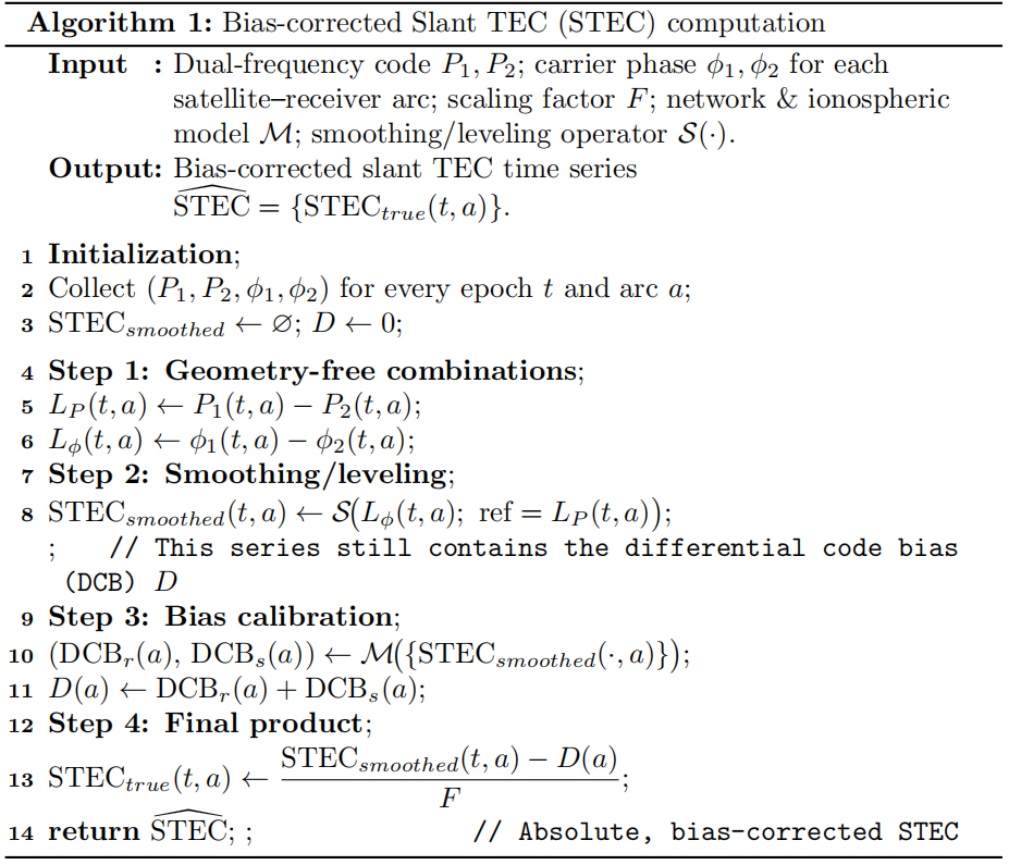
Algorithm 1.
Currently, the most reliable reanalysis model and data source for the ionosphere are the global ionospheric TEC maps provided by the International GPS Service (IGS), which offer more than 20 years of stable data[92]. These maps are generated using multi-frequency and multi-constellation satellite navigation observations from over 500 stations worldwide, and the data are processed through reanalysis or assimilation models that employ polynomials and spherical harmonics. The resulting models produce global ionospheric TEC maps with a temporal resolution of approximately 2 h and a spatial resolution of 5° in longitude and 2.5° in latitude. Among the seven global data analysis centers authorized by IGS, the Technical University of Catalonia (UPC), the Chinese Academy of Sciences (CAS), and Wuhan University (WHU) have begun providing near-real-time Global Ionospheric Maps (GIM) products[93]. As a result, the temporal resolution of GIM can be further reduced to intervals such as 5 min, 15 min, or 1 h[94-97].
Additionally, many Continuously Operating Reference Stations (CORS) are distributed globally, with station spacing ranging from tens of kilometers to hundreds of kilometers. CORS are used for various applications, including geological monitoring, ionospheric and tropospheric parameter inversion, and serving as the foundation for precise point positioning and real-time kinematics (RTK)[98]. CORS data have been instrumental in studying ionospheric co-seismic effects. For example, following the 2022 Tonga volcanic eruption, researchers used CORS data from around the world to replicate the ionospheric Lamb waves and bowl waves induced by the eruption[99-103]. Furthermore, CORS observations from Japan and Taiwan (China) have provided valuable insights into the multi-layer coupling effects within the Earth during the 2011 Tohoku Earthquake[104]. Satellite navigation observation networks, both global and regional, focus on studying the effects of ionospheric scintillation caused by the formation of ionospheric irregularities. Notable examples include the Canadian High Arctic Ionospheric Network (CHAIN, http://chain.physics.unb.ca/chain/)[105], the Concept for Ionospheric Scintillation Mitigation for Professional GNSS in Latin America (CIGALA), and the Countering GNSS High Accuracy Applications Limitations Due to Ionospheric Disturbances in Brazil (CALIBRA, https://ismrquerytool.fct.unesp.br/) networks in South America[106]. Ionospheric irregularities primarily occur in the global EIA and high-latitude regions. The EIA mainly causes amplitude scintillation in satellite signals, while high-latitude regions predominantly affect satellite navigation signals through phase scintillation. Due to the global distribution of geomagnetic latitudes and longitudes, the South American region, especially Peru and Brazil, experiences the most severe ionospheric scintillation effects in low-latitude areas, while the Canadian region in North America represents high-latitude areas. In these regions, both conventional satellite navigation receivers and specialized ionospheric scintillation receivers are deployed. For example, the Low-latitude Ionosphere Sensor Network (LISN, http://lisn.igp.gob.pe/about/detail/institutional/) serves as an observation network in these areas[107]. The characteristics of above-ground observation networks can be summarized as follows: (1) These networks offer multiscale spatial coverage. For example, the International GNSS Service (IGS) operates global ground observatories, while many regional CORS networks are found in countries such as the United States (https://www.ngs.noaa.gov/CORS/), Italy (https://webring.gm.ingv.it/), Germany (https://igs.bkg.bund.de/root_ftp/), Japan (http://terras.gsi.go.jp/), and China (CMONOC, Crustal Movement Observation Network of China[108]); (2) Oceanic regions are not covered, primarily due to the challenges of establishing stable observatories on the sea surface; (3) There is a hemispheric imbalance in the density of deployments, with a higher concentration along geomagnetic latitudes in the Northern Hemisphere, while the Southern Hemisphere has fewer regional GNSS networks. Notable exceptions include Brazil (http://geoftp.ibge.gov.br/), Australia (http://ga.gov.au/), and New Zealand (https://www.geonet.org.nz); (4) There is also a geopolitical disparity, with dense networks in developed countries, ensuring high data quality and network stability, while deployments in certain regions of Africa remain sparse. In addition, other low Earth orbit (LEO) ionosphere observables have highlighted the limitations of the IRI model in modeling the topside ionospheric profile. With the aid of the Alouette and International Satellites for Ionospheric Studies (ISIS) topside sounders, as well as in-situ radio occultations from the Challenging Minisatellite Payload (CHAMP) and the Gravity Recovery and Climate Experiment (GRACE), the topside ionospheric plasma density has been significantly corrected and refined[109]. Comprehensive comparisons of satellite-based plasma density observations considering data from the Constellation Observing System for Meteorology, Ionosphere, and Climate (COSMIC), CHAMP, GRACE, the Communications/Navigation Outage Forecasting System (C/NOFS), and Swarm are essential for further model improvements[110,111]. These data, particularly from occultation measurements, demonstrate significant spatiotemporal discontinuities. The spatial sampling density of these observations depends on the configuration of the satellite constellations. Nevertheless, the altitude-specific ionospheric electron density and TEC data provided by satellite-based observations, when effectively integrated with ground-based data and existing models, offer valuable insights into new phenomena and mechanisms related to the 3D evolution of ionospheric TEC[112].
The first phase of the COSMIC, which was a collaborative project between the U.S. National Center for Atmospheric Research and Taiwan, was launched in 2006. This system consists of six small satellites, each equipped with occultation instruments capable of obtaining vertical profiles of key atmospheric parameters in both the ionosphere and troposphere. Since 2009, stable and continuous COSMIC data have been made available[113-115]. The system’s primary and secondary data products include ionospheric electron density profiles, TEC, and the ionospheric scintillation index, providing a crucial observational foundation for studying the 3D variations of global ionospheric TEC. The second phase of COSMIC, which began construction in 2019, aims to create a global constellation of 18 low-Earth orbit satellites. This expansion is expected to triple the number of occultation events observed globally within a 2-h period, resulting in a denser, more comprehensive 3D sampling network for ionospheric electron density and TEC[116-118].
C/NOFS satellite was a pioneering mission designed to study ionospheric irregularities and their impact on communication and navigation systems[119]. Developed through a collaboration between the U.S. Air Force Research Laboratory (AFRL) and National Aeronautics and Space Administration (NASA), C/NOFS aimed to predict ionospheric scintillations and disturbances that can disrupt radio signals and GPS accuracy. Launched in 2008 and operational until 2015, its data continues to contribute significantly to space weather research. During the unusually deep solar minimum of cycle 23/24, C/NOFS data revealed unique ionospheric behaviors, such as reduced plasma densities and altered irregularity patterns, providing insights into solar-cycle dependencies. The Swarm satellite constellation, launched by the European Space Agency (ESA) in 2013, represents a groundbreaking mission designed to study Earth’s magnetic field and its interactions with the ionosphere and space weather[120]. Comprising three identical satellites, Swarm provides unprecedented high-precision measurements that have revolutionized our understanding of geophysical processes and space weather phenomena. This comprehensive overview covers the mission’s design, instrumentation, and its critical applications in ionospheric and space weather research. Through its innovative multi-satellite design and sophisticated instrumentation, Swarm has enabled breakthroughs in ionospheric tomography and the study of plasma irregularities, Space weather forecasting and geomagnetic storm monitoring, Coupling processes between the atmosphere, ionosphere, and magnetosphere.
In addition to ground-based and space-based ionospheric observations, incoherent scatter radar (ISR) observations are essential for probing the ionosphere. The thermal motion of medium-density plasma in the ionosphere results in Thomson scattering of incident electromagnetic waves, which is exploited by ISRs. Since the 1960s, the United States and the European Incoherent Scatter Scientific Association (EISCAT) have established more than ten ISRs[121]. In China, supported by the Chinese Meridian Project, the Qujing Incoherent Scatter Radar (QJISR) was constructed in Yunnan Province in 2012, followed by the recent completion of the Sanya Incoherent Scatter Radar (SYISR)[122,123]. ISRs can measure electron density, electron and ion temperatures, plasma drift velocity, and can indirectly infer ionospheric conductivity, electric fields, thermospheric winds, and particle collision frequencies. These radars offer high temporal resolution, often on the order of tens of seconds, and spatial resolution on the scale of hundreds of meters. The Millstone Hill ISR in the United States has been in operation for nearly 50 years and has contributed to the development of the Madrigal global ISR data-sharing system (Madrigal, madrigal.haystack.mit.edu).
Significant progress has been made in understanding ionospheric characteristics and models in the mid-latitude and auroral regions. The European EISCAT team developed the Ground-based Incoherent Scatter Data Analysis and Processing software (GUISDAP), which focuses on the structure, climatology, disturbances, and electrodynamics of the high-latitude ionosphere in the Nordic region[124]. The Qujing and Sanya ISRs, located in the low-latitude regions of China, provide valuable insights into the formation, evolution, and structural morphology of non-uniform ionospheric structures in the mid- and low-latitude regions[124,125]. Additionally, the Jicamarca ISR in Peru, situated at even lower latitudes, has been instrumental in discovering ionospheric irregularities with spatial scales as small as three meters[126]. This research has revealed the mechanisms behind the development and evolution of plasma instability in low-latitude and equatorial regions, significantly advancing the understanding of equatorial ionospheric electrodynamics.
3. ADOPTABLE DL APPROACHES
Modern AI modeling approaches, particularly those utilizing ML and DL networks, are increasingly applied to model the ionosphere at both global and regional scales. DL, with its strong capability for nonlinear function approximation, offers an effective complement to the limitations of traditional physical and empirical models. Recent advancements in DL techniques have introduced new perspectives for ionospheric modeling and prediction, suggesting that AI methods hold significant potential for spatial and temporal geoscience modeling and future research[127]. Similar to their use in computer vision and natural language processing, convolutional neural networks (CNNs), recurrent neural networks (RNNs), and generative networks are now being explored to address spatiotemporal, multiscale space physics challenges. These include tasks such as ionospheric anomaly detection, feature extraction, physical phenomenon identification, and multiscale temporal prediction[128,129]. In addition, substantial breakthroughs in AI applications within meteorology have demonstrated that transformer-based DL models can outperform traditional methods in spatiotemporal prediction, reanalysis modeling, and nowcasting[130-132], providing promising cases for AI-assisted ionospheric modeling.
The GIM products provide a continuous and stable dataset for investigating global ionospheric morphology. With over twenty years of data, they are highly suitable for AI-based ionospheric modeling and prediction. Additionally, other ground-based and space-borne ionospheric observations, as discussed in Section 2, can also be utilized for ionospheric modeling, spatiotemporal estimation, and anomaly detection.
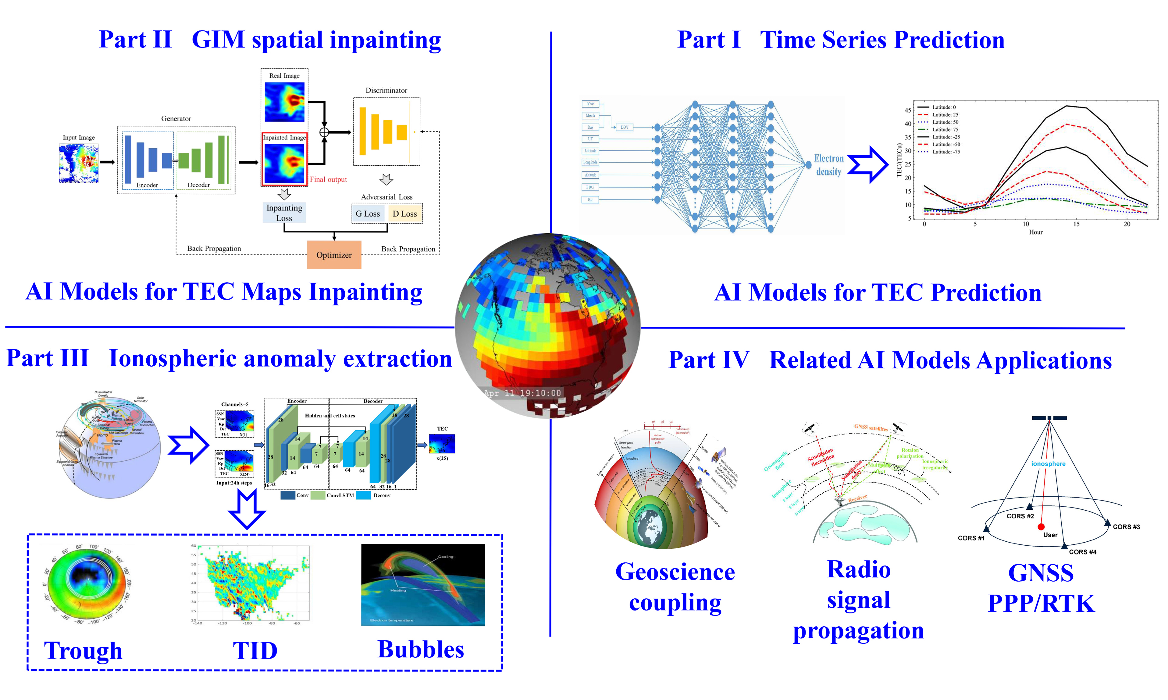
Recent advances in AI-driven ionospheric studies primarily focus on using DL networks for modeling and predicting the temporal and spatial variations of ionospheric TEC. Some studies also concentrate on ionospheric anomaly feature detection and extraction, as summarized in Figure 2.
Figure 2. The adoptable deep learning approaches in ionosphere studies. GIM: global ionospheric maps; TEC: total electron content; TID: traveling ionospheric disturbance.
3.1. Temporal ionosphere modeling with DL networks
Ionospheric prediction in the temporal domain has long been a subject of significant interest, as shown in Figure 3. RNNs, such as long short-term memory (LSTM), Gated Recurrent Units (GRU), and attention-based backbone neural networks, have proven effective for forecasting key ionospheric parameters. These include the foF2, TEC, and electron density profiles, which can be predicted over both short-term (hours) and medium-to-long-term (days to weeks) time frames. For foF2 prediction, Bi et al. utilized the Informer framework to achieve long-term, effective forecasting[133]. For TEC prediction, numerous studies have been conducted, typically employing datasets gathered from global satellite navigation systems[133].
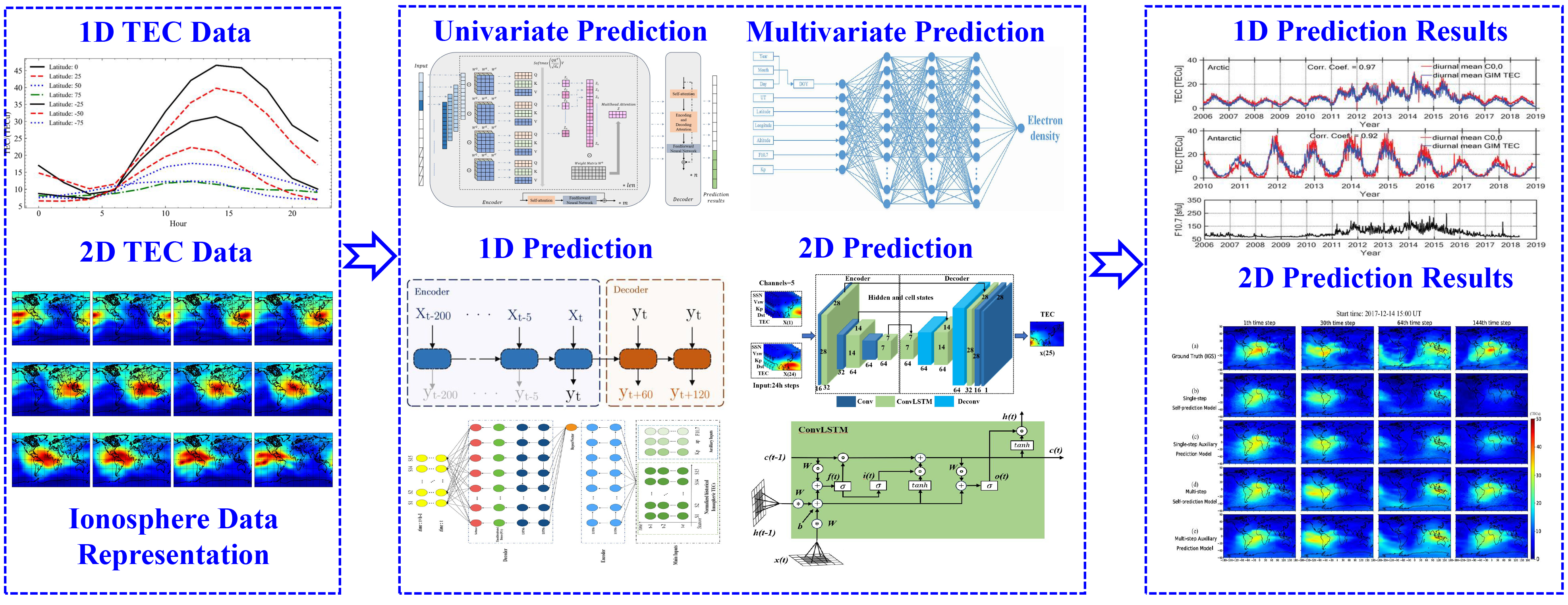
Figure 3. Temporal prediction of ionospheric TEC with ML and DL frameworks. 1D: One-dimensional; TEC: total electron content; 2D: two-dimensional; ML: machine learning; DL: deep learning.
LSTM networks are commonly used as the framework for constructing short-term prediction models of global ionospheric TEC, typically in one-dimensional (1D) or 2D formats. However, prediction accuracy tends to decrease as the output time step increases[108-110,133-135]. For medium- and long-term predictions, attention-based mechanisms and transformer-based frameworks have become more prevalent as backbone networks[109-111,133,135,136]. Bi et al. (2022) applied an Informer model, notable for its efficient attention mechanism, to successfully forecast the critical frequency foF2 in mid-latitude regions[133]. Similarly, Lin et al. (2022) developed an optimized transformer model utilizing positional embedding to improve the prediction accuracy of one-dimensional TEC time series[135]. Expanding this to 2D forecasts, Xia et al. (2022) proposed the CAiTST model, which innovatively integrates convolutional neural networks with a transformer to process and predict full TEC maps by capturing both spatial features and temporal dynamics[136]. Collectively, these studies highlight the growing efficacy and adaptability of attention-based deep learning models in addressing key ionospheric parameter prediction tasks.
In the study of the topside ionosphere, several studies have focused on modeling and predicting electron density profiles. Using radio occultation observations from COSMIC, a four-dimensional physical grid model of ionospheric electron density was developed using deep neural networks[129]. Similarly, a study by Smirnov et al. utilized 19 years of GNSS radio occultation data to model topside ionospheric electron density with a neural network[111]. This AI-based model outperforms the state-of-the-art IRI model, particularly in the 100 to 200 km range above the F2 layer peak. The results demonstrate that data-driven models of topside ionospheric electron density reveal complex physical processes that govern topside dynamics. Additionally, radio occultation observations provide a reliable data source for 3D modeling of ionospheric electron density. As mentioned in introduction part, data assimilation strategies have been applied for 3D ionospheric modeling, laying a solid foundation for state-of-the-art comparison metrics in potential 3D modeling using DL networks[113-117,137-142].
Transition from traditional machine learning to DL in Ionosphere temporal prediction
Traditional ML methods were adopted in the early stage of ionosphere temporal prediction. For instance, linear regression, random forest, XGBoost and light gradient boosting algorithm (LightGBM) algorithms are considered as ways to improve short term ionosphere morphology prediction. Tang et al. applied random forest to ionosphere vertical plasma drift prediction, with precise capability to capture the climatological variations for equatorial ionosphere vertical plasma drifts[143]. It demonstrated superior performance in high dimensional nonlinear modeling for ionosphere vertical drifts than other methods. Shidler et al. used LightGBM to predict ionospheric TEC in low latitudes during storm times, indicating higher prediction accuracy than the IRI model[144]. Nigusie et al. evaluated two types of framework of ionosphere TEC prediction under geomagnetic disturbances, one is light gradient boost machine (LGB) and the other is deep neural network (DNN)[145]. Han et al. develops a global ionospheric slab thickness prediction model by integrating XGBoost with Ensemble Learning (EL). The model utilizes inputs such as vertical TEC, solar flux (F10.7), and geomagnetic indices (Ap, Dst), achieving superior accuracy over the Neustrelitz Slab Thickness Model and the International Reference Ionosphere[146]. Traditional ML methods have some inherent limitations in ionospheric prediction modeling: (1) Traditional ML relies much on feature engineering, which serves as a typical characteristic of ML; however, in face of complex ionosphere spatial and temporal variations, it requires much complicated artificial settings, especially to deal with the space physical influences on ionosphere; (2) Ionosphere exhibits strong nonlinearity and nonstability during disturbance, such as ionosphere storms, while it is hard for traditional ML methods to demonstrate or represent correctly those dynamic evolutions in ionosphere; (3) Traditional ML methods are weak to deal with high dimensional data, while modern ionosphere data contain diverse types of observations from both ground stations and space satellites, thus leading to the dilemma of dimensional explosion and information loss; (4) Traditional ML methods lack externalization and generalization capabilities under extreme events, such as strong ionospheric storms; (5) These methods, especially the tree-like models, are limited in representation capability and flexibility; in contrast, DL neural networks such as CNNs can well approximate most complex functions.
To address the above limitations for traditional ML methods, especially those tree-like models, recent studies apply DL frameworks in ionosphere temporal and spatial prediction modeling, which will be discussed in detail below.
3.1.2. Ionosphere temporal prediction with single and multiple physical parameters
Ionospheric temporal prediction can be approached using a single parameter, where only one ionospheric parameter, such as TEC or the foF2, is used as input to DL networks. Several previous studies have focused on this approach. For example, recently proposed frameworks such as multi-strategy assisted osprey optimization algorithm (MAOOA)-residual-attention-bidirectional convolutional LSTM (BiConvLSTM), Encoder-Decoder-AttentionConvLSTM (ED-AttentionConvLSTM), and Encoder-Decoder-ConvLSTM (ED-ConvLSTM) have been developed. LSTM networks have been shown to play a significant role in ionospheric temporal modeling and prediction[145-150,117,118]. However, as noted earlier, LSTM models face limitations in medium- and long-term prediction tasks. To address this, several encoder-decoder-based prediction networks have been adopted. For instance, a self-attention mechanism within a transformer framework has been applied to capture long-term variations in TEC in China, outperforming the LSTM framework by 23% for the period from 2016 to 2018[110].
In the aforementioned cases, the structure of the DL network, along with the selection of hyperparameters, plays a critical role in the performance of ionospheric prediction tasks. Specifically, the number of hidden layers and the number of training iterations must be carefully chosen to optimize model performance. For instance, an excessively large number of training iterations can lead to overfitting, while too few iterations may result in underfitting, causing large prediction errors[140].
As is well known, ionospheric variation is influenced by multiple space physics factors, including solar radiation flux (F10.7 index), sunspot number (R), geomagnetic index (Ap), and geomagnetic storm index (DST). When appropriately incorporated, these factors can improve the accuracy of ionospheric modeling[137,138]. The coupling mechanism between these factors and ionospheric TEC has been explored using statistical correlations and various ML approaches[139]. However, the challenge in temporal modeling and prediction of the ionosphere using multiple space physics parameters lies in the complex interactions between factors such as F10.7, R, Ap, DST, and ionospheric TEC. Specifically, the internal physical links between solar activity, geomagnetic activity, and ionospheric variation remain difficult to fully characterize and model.
3.1.3. Ionosphere temporal prediction with 1D and 2D data frameworks
Ionospheric temporal prediction methods can be categorized into 1D and 2D approaches based on how the dataset is processed. As mentioned in Section 2, most ionospheric observations, whether ground-based or space-borne, are typically represented as Euclidean data. Depending on the source of the observations, ionospheric variation can be described either as a 1D array or a 2D figure, which incorporates both temporal and spatial features of the ionosphere. For 1D data prediction, temporal variations and fluctuations of the ionosphere are modeled using 1D neural network architectures, such as traditional LSTM, attention-based LSTM, the original transformer, Informer, Autoformer, and TimesNet. However, 1D data prediction does not account for spatial correlations in the ionosphere, which is a key feature in geoscience problems. To address this limitation, some researchers have turned to 2D data representations. For instance, GIM data are gridded to ensure good temporal and spatial consistency, which generates 2D ionospheric features. The processing of 2D ionospheric datasets is similar to image processing. For example, a convolutional-attentional image time-sequence transformer (CAiTST) was proposed to predict ionospheric TEC maps at different solar activity levels for one-day intervals. Results show that CAiTS outperforms the 1-day Center for Orbit Determination in Europe (CODE) prediction[108,109,135,137]. Additionally, several DL frameworks, such as MAOOA-Residual-Attention-BiConvLSTM, ED-AttConvLSTM, and ED-ConvLSTM, are all designed for 2D ionospheric temporal prediction.
Spatial ionosphere modeling with DL networks
The ionospheric observations discussed in Section 2 have inherent limitations in their spatial distribution. For example, ground-based ionospheric observations often exhibit uneven coverage, with gaps over oceans. In contrast, space-borne observations are discontinuous in both the temporal and spatial domains. These limitations hinder a more detailed understanding of fine ionospheric structures, particularly in regions such as the EIA, TIDs, and ionospheric irregularities. To address these challenges, one potential solution is the application of generative adversarial networks (GANs). First proposed by Goodfellow in 2014[151], GANs have proven highly effective in various applications, including data augmentation and image restoration. A GAN consists of two primary components: a generator network and a discriminator network. The generator network learns to approximate the statistical distribution of the target data by using its "imitation" ability to transform random input sequences into realistic outputs. In contrast, the discriminator network aims to differentiate between the generator’s output and the true target data, effectively assessing the quality of the generated data. During the training process, the discriminator is first trained using an upward gradient strategy, followed by training the generator with a downward gradient strategy. This iterative process continues until the generator and discriminator reach an equilibrium state, where the discriminator can no longer distinguish between the generator’s output and the real data, resulting in a discriminator loss function of 0.5.
GANs have been employed for ionospheric TEC completion and reconstruction, providing a broader spatial coverage of TEC distribution. Ji et al. utilized conditional GANs to enhance the output accuracy of the IRI model[152]. The deep convolutional GAN (DCGAN) was adopted to improve TEC completion accuracy, particularly in regions with significant data gaps. To supplement coverage in oceanic areas, Massachusetts Institute of Technology (MIT) global TEC map products were augmented using DCGAN and spectral normalized patch generative adversarial network (SNPGAN)[153-157]. The completion root mean square error (RMSE) achieved was below 2 TECu during geomagnetically quiet periods and less than 4 TECU during geomagnetic storms. Jeong et al. applied DCGAN with Poisson blending for fine-grained modeling of the local ionosphere in South Korea[154]. Yang and Liu compared the performance of DCGAN and Wasserstein GAN with Gradient Penalty (WGAN-GP) networks for global TEC data augmentation, testing these models under both geomagnetically quiet and disturbed conditions[158]. Figure 4 illustrates the general framework for spatial modeling and data completion of ionospheric TEC, showcasing a typical GAN structure. The input of 2D TEC data is represented as images, with two primary components in the network: the generator and the discriminator. The generator is typically modeled using an encoder-decoder network, while the discriminator functions as a classifier. For optimal network performance, both the generator and discriminator have separate loss functions.
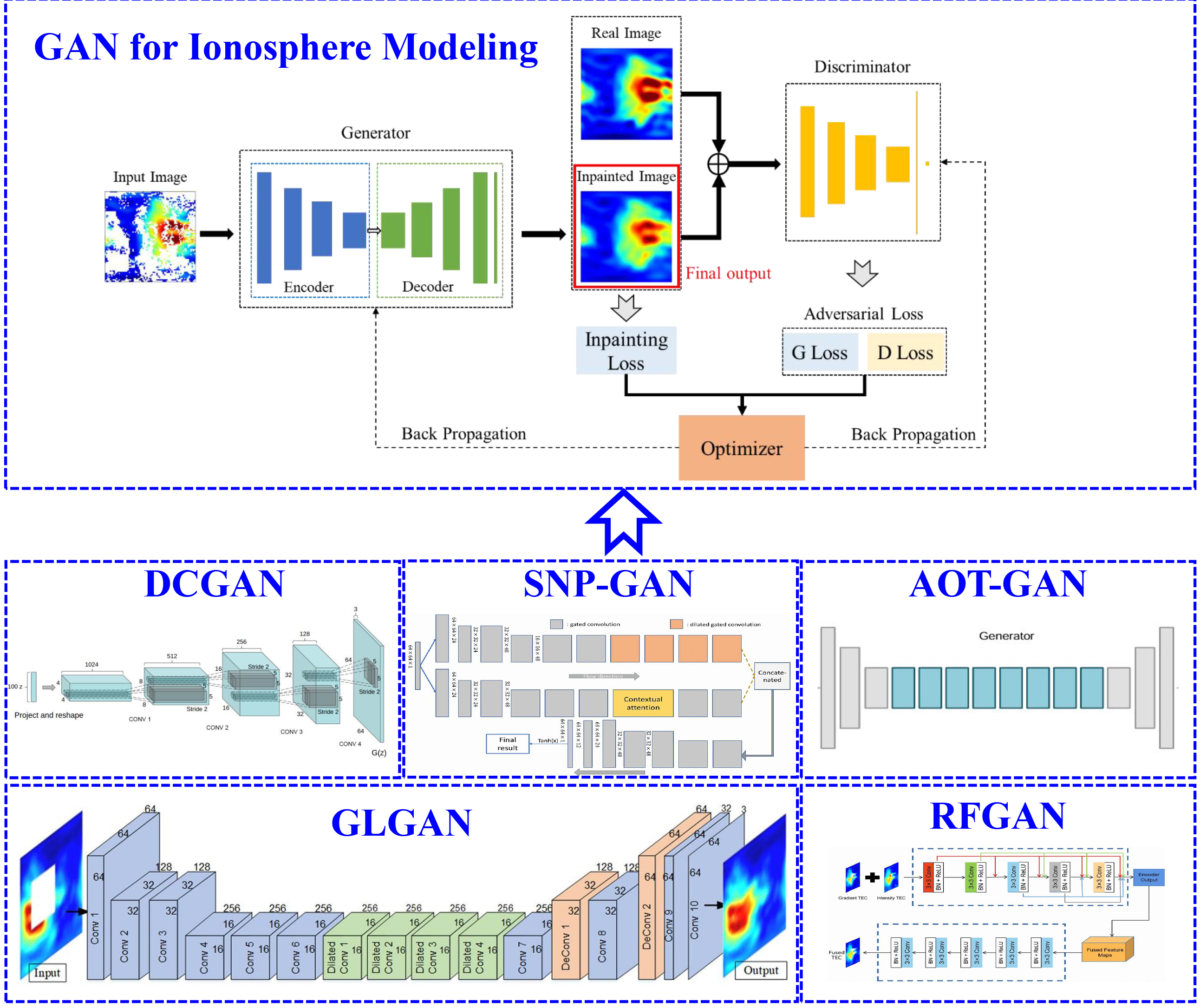
Figure 4. Spatial modeling and data completion of ionospheric TEC with DL frameworks. GAN: Generative adversarial network; DCGAN: deep convolutional generative adversarial network; SNP-GAN: spectral normalized patch generative adversarial network; AOT-GAN: aggregated contextual-transformation generative adversarial network; GLGAN: Global and Local GAN; RFGAN: a deep learning hybrid model; TEC: total electron content; DL: deep learning.
3.3. Applications of DL in other ionosphere studies
Spatiotemporal modeling of ionospheric TEC offers insights into the macroscopic evolution of the ionosphere’s behavior. However, at regional scales, specific ionospheric features, including TIDs, ionospheric irregularities, ionospheric troughs, and co-seismic ionospheric disturbances (CIDs), display distinct patterns that require further investigation. Several DL networks originally developed for computer vision and pattern recognition[159] have been applied to study these specific patterns.
Lan et al. employed a convolutional neural network (CNN) with a 5 × 5 kernel size to extract feature maps for automatic spread-F identification[160]. For training, they used ionograms recorded in 2015 and July 2016, comparing the performance of CNN with other ML methods, such as decision trees and random forests. Their results demonstrated that CNN outperformed the other methods, showing considerable potential for recognizing ionospheric spread-F patterns[160].
Tian et al. applied a 3D U-Net to extract the latent relationship between bottom ionospheric winds and temperature, and the sporadic E layer. They trained the model using the 5th generation of European ReAnalysis (ERA5) reanalysis data and COSMIC radio occultation data[161]. The 3D U-Net, an improved version of the original U-Net, is designed for semantic segmentation, consisting of a contracting encoder and an expanding decoder for full-resolution segmentation[162]. Their study highlighted the strong potential of DL networks in uncovering the complex coupling mechanisms responsible for ionospheric irregularities in the E layer.
A Mask Region-Convolutional Neural Network (R-CNN) was employed to detect wave-like perturbations in Medium-Scale Traveling Ionospheric Disturbances (MSTIDs) over Japan. The training dataset consisted of GPS-TEC data provided by the GPS Earth Observation Network (GEONET) in Japan[162]. The network structure includes a feature extraction network, a region proposal network (RPN), region-of-interest (ROI) selection, normalization, and prediction regression. The upward and downward arrows in the feature extraction network represent down-sampling and up-sampling, respectively. The MSTID wave structures were clearly visible in the differential TEC (dTEC) maps, which served as the primary image source for the training data. In total, 1,209,600 images from 1997 to 2019 were used. The dTEC maps were categorized into two groups, namely daytime and nighttime data. Both groups were trained and tested using the ResNet-50/ResNet-101 network backbones, and six different waveforms were output as categories. Statistical analysis was performed to explore the relationship between MSTID occurrences and solar and geomagnetic activity.
To construct a more robust model, a dataset of airglow images observed in China from October 2011 to December 2021 was compiled for training. The output of the CNN was classified into five categories, with only one category selected for further identification of MSTID[163]. The model achieved a classification accuracy of 96.9% and a localization accuracy exceeding 70%. Using this model, the periodic MSTID occurrence ratio at the Xinglong station in China was calculated for the period between 2012 and 2021.
An automatic co-seismic ionospheric disturbance (CID) classification model was developed using a random forest algorithm[164]. This model, which uses TEC waveform data as input, can automatically recognize CID patterns and estimate arrival times within 15 min of a seismic event. Trained on CID datasets from 12 earthquake events, the model achieved a classification accuracy of 96% and an arrival-time accuracy of less than 20 s. Additionally, semi-supervised ML algorithms were applied to monitor Traveling Ionospheric Disturbances (TIDs) and sporadic E layers (Es) globally, utilizing space-borne GNSS-radio occultation (RO) measurements.
In summary, DL networks play a crucial role in pattern recognition and feature extraction for the study of ionospheric irregularities, MSTIDs, CIDs, and other ionospheric anomalies. These automated and intelligent methods greatly enhance statistical analyses of occurrence patterns and provide deeper insights into the latent coupling mechanisms governing ionospheric behavior.
3.4. Performance evaluation for successful DL ionospheric modeling
Several critical factors contribute to the success of ionospheric modeling using DL networks: reliable datasets, accurate and robust network models, and a comprehensive understanding of ionospheric physics. High-quality ionospheric observation data primarily come from remote sensing methods, including satellite navigation systems, ISRs, and optical imaging techniques. Ground-based observations offer the advantage of long-term, continuous data collection, but they are often limited by uneven global spatial coverage. In contrast, space-borne observations provide valuable data but are inherently subject to spatiotemporal discontinuities, making it difficult to obtain complete 3D observations on a global scale.
From the perspective of model training, several challenges must be addressed: (1) the ability to describe the spatiotemporal evolution of ionospheric irregularities based on current data sources; (2) the capacity to capture the features of the topside ionosphere with existing observations; (3) the ability to identify multiscale spatial structures within the ionosphere; and (4) the capacity to predict ionospheric variations both in the near term and over extended periods. These capabilities can be realized using different DL network architectures. For instance, RNNs, such as LSTM, GRU, and the attention-based networks such as Transformer, Informer, and PatchTXT, have demonstrated efficient performance in the temporal prediction of ionospheric variations. Similarly, GANs such as DCGAN, SNPGAN, Wasserstein GAN (WGAN), and aggregated contextual-transformation GAN (AOT-GAN) are particularly well-suited for spatial data augmentation in ionospheric observations. Specific ionospheric patterns, such as spread-Es, equatorial plasma bubbles, and MSTIDs, require advanced semantic segmentation networks for precise and automated feature extraction.
Moreover, with the development of large language models (LLMs) and generative AI [AI-generated content (AIGC)], there is potential to construct a spatiotemporal ionospheric model based on LLMs or generative AI. However, challenges remain in generating a foundation model for ionospheric modeling and prediction, especially when compared to established foundational models for the troposphere, such as GraphCast, GenCast and Pangu[165-168]. A primary obstacle is the lack of continuous spatiotemporal 3D observations of ionospheric TEC or electron density. In contrast, for weather forecasting, comprehensive reanalysis datasets from the European Centre for Medium-Range Weather Forecasts (ECMWF) are readily available. The topside ionosphere, spanning the vertical range up to 1,000 km, has limited observational data, and even in the bottom-side ionosphere, available data are relatively sparse, primarily consisting of spotty ground-based ionosonde and ISR measurements. As a result, ionospheric sensing coverage still needs to be extended and augmented, posing significant challenges to developing a comprehensive ionospheric model across the entire altitude range[92].
The advantages of using DL for ionospheric modeling and forecasting lie in the ability of modern DL networks to automatically and more accurately extract ionospheric features. Numerous studies have compared the accuracy of ionospheric TEC predictions between DL models and traditional methods, including ML approaches such as random forest, LightGBM and XGBoost. DL frameworks, particularly LSTM and attention-based models, have shown significant improvements in short- and medium-to-long-term TEC prediction. For spatial modeling, generative DL networks, such as GANs, variational autoencoders (VAEs), and diffusion models, have proven highly effective for data augmentation. These models outperform traditional methods such as polynomial and kriging interpolation, making them a promising approach for ionospheric spatial modeling and prediction.
It is also important to note that certain data assimilation algorithms, such as the Ensemble Kalman Filter, have demonstrated strong performance in ionospheric modeling. As such, the potential for fusing ionospheric observations with DL networks, whether in single-modal or multi-modal settings, deserves significant attention.
These frameworks, originally developed for tasks in computer vision and large language modeling, may offer considerable promise for improving ionospheric forecasting capabilities.
Table 2 presents a comparison of ionospheric prediction performance between various methods, highlighting the advantages of DL networks over traditional approaches.
Comparison of ionosphere prediction performances
| Author | Model | RMSE(TECu) | R 2 | ||||
| High solar activity year | Low solar activity year | High solar activity year | Low solar activity year | ||||
| IRI[31] | IRI-2016 | 11.516 | 4.720 | 0.640 | 0.476 | ||
| CODE[92] | COPG | 4.855 | 1.794 | 0.936 | 0.924 | ||
| Xia et al.[148] | ED-ConvLSTM | 4.708 | 1.645 | 0.940 | 0.936 | ||
| Li et al.[149] | ED-AttConvLSTM | 4.613 | 1.610 | 0.944 | 0.939 | ||
| Wang et al.[150] | MAOOA-Residual-Attitude-BiConvLSTM | 3.855 | 1.418 | 0.943 | 0.944 | ||
3.5. Interpretability of DL ionosphere models
From the perspective of the physical nature of the ionosphere, several challenges remain in improving the accuracy and performance of ionospheric modeling: (1) The predictive capability of TEC in the EIA region requires further improvement[169]. Due to increased fluctuations in this region, data-driven methods, particularly those based on DL, struggle to effectively capture these variations; (2) TEC prediction during geomagnetic storms and other space weather events needs significant enhancement. Current DL-based approaches mainly rely on historical TEC data to identify fluctuation patterns. However, geomagnetic storms typically last only a few days to a week, resulting in limited data for training. This data scarcity hinders the model’s ability to learn and capture the full extent of ionospheric instability during such short-duration events. Additionally, ionospheric perturbations caused by geomagnetic storms are characterized by inherent uncertainty and randomness, further complicating accurate modeling.
Because of their large number of parameters and often complex architectures, DL models are commonly regarded as “black-box” techniques. When applied to specific scientific fields, such as space physics, it is crucial that the performance of the chosen DL networks aligns with the physical mechanisms of the ionosphere. In this context, DL models in space physics must be interpretable, both in terms of the model structure and the training procedures.
An interpretable DL model is one that is self-consistent, similar to supervised regression or decision trees, where explicit parameters describe the model’s operation. To some extent, attention mechanisms can also serve as an interpretable component within these DL models, as they have a clear mathematical definition. However, some DL networks used in ionospheric modeling are more interpretable based on factors such as the choice of training hyperparameters and strategies, feature map extraction, knowledge distillation, activation function selection, and the flow of information within the network.
The tuning of hyperparameters here consists of two parts as indicated in Table 3. In Table 3, (1) The automatic tuning, which is adopted for all DL frameworks. During training procedure, automatic tuning is used for weighting factors optimization, and those optimization methods are considered, such as grid searching, random searching, Bayesian optimization as well as evolutionary algorithms; (2) Tuning by knowledge in the field, here referring to knowledge and principal theory in ionosphere physics. For instance, the input time window should cover the critical period of the ionosphere, including daily or monthly variation periods; the size of the convolutional core should match the spatial correlation scale of the ionosphere TEC; the sensitivity of storm events should be considered with larger model capability and normalization strength.
Tuning strategies for ionosphere DL models
| Challenges | Tuning strategy |
| Daily/seasonal variations | Enlarge the layers of LSTM/Transformer, increase the length of input time window, use attention mechanism to capture critical epochs |
| Spatial heterogeneity, difference between equatorial and polar regions | Regional modeling by training in different latitudes, applying GNN to demonstrate spatial correlations |
| Extreme events forecast, such as geomagnetic storms forecast | Enlarge model volume and parameters, add more event detection models, modify loss functions |
| Unbalanced data distribution, deficiency in ocean and desert | Use spatial interpolation pre-training, apply GAN framework to make data augmentation |
| Multiple data fusion, GNSS/COSMIC/Swarm/GIRO | Design multi-modal inputs, adjust weighting parameters for different data sources |
The efficiency of hyperparameter tuning can be verified through spatial and temporal cross-validation. To ensure a rigorous and consistent cross-validation, temporal information should be preserved. For instance, the time spans of training, testing, and validation datasets should be kept separate. Spatial generalization should also be validated, for example by testing performance in different regions of the Earth. Finally, the extreme events such as geomagnetic storms should be carefully handled and isolated during training, testing and validation. Table 4 shows some tuning strategies for ionosphere DL models.
Ionosphere modeling tasks and related DL solutions
| Task | Solved problem | Methods | |
| Ionosphere temporal modeling | Univariate | Only known TEC predicts future TEC | (Kaselimi et al.[171]) (Chen et al.[174]) (Chen et al.[175]) (Xia et al.[148]) (Xia et al.[136]) (Bi et al.[133]) (Li et al.[149]) (Wang et al.[150]) |
| Multivariable | Known TEC + physical parameters predict future TEC | (Liu et al.[170]) (Kim et al.[172]) (Xiong et al.[173]) (Xie et al.[176]) (Gao et al.[177]) (Lin et al.[135]) (Tang et al.[178]) (Ren et al.[179]) | |
| Ionosphere spatial modeling | Data Augmentation Spatial TEC map completion | (Chen et al.[153]) (Ji et al.[152]) (Pan et al.[155]) (Chen et al.[156]) (Pan et al.[157]) (Yang et al.[180]) (Chen et al.[181]) | |
| Ionospheric anomaly extraction | Detection and analysis of TIDs | (Liu et al.[162]) (Lai et al.[163]) | |
With the systematic hyperparameter adjustment mechanism, the accuracy, robustness and physical rationality of DL model in complex ionosphere TEC prediction task can be significantly improved, especially in capturing sudden space weather events, which surpasses traditional methods.
The mathematical foundation of DL is largely based on the universal approximation theorem and the Kolmogorov-Arnold representation theorem[147]. Most current DL models employ gradient-based optimization techniques, which typically lead to local optima in the optimization process. Due to the non-convex nature of these models, different optimal solutions may be found depending on how the network is trained, influenced by variations in the training data and parameter strategies.
Generative models, as discussed above, are unsupervised but can be partially interpreted through optimal transportation theory. This theory facilitates the mapping of data across different latent spaces, establishing correspondences and substitutability. In generative models, the metric used to measure the similarity between source data and the transformed data is critical. For example, the Wasserstein distance, used as a loss function in GANs, offers a new perspective for evaluating the mapping performance across different latent spaces. For most data in Euclidean space, metrics such as cross-entropy, Kullback-Leibler divergence, and Jensen-Shannon divergence are commonly considered.
Ionospheric observations can be treated either as Euclidean data or transformed into other data types, such as graph data. In the approaches discussed for ionosphere modeling, ionospheric observations are typically treated as stable time series in Euclidean space. However, when adjacent connections and spatial dependencies across different regions are considered, the data can be treated as graph data. In such cases, appropriate graph neural networks should be applied to address the problem effectively.
3.6. AI ionosphere modeling with integration of physics information
It is crucial to assess the impact of heterogeneous observations with varying spatial and temporal scales on the accuracy of ionospheric modeling. In regions of high and mid-latitudes, where ground-based ionospheric observations are more abundant, the influence of solar activity and the geomagnetic field on ionospheric variations is relatively straightforward and easier to interpret. In contrast, low-latitude regions exhibit more complex ionospheric behavior, with significant variations in both spatial and temporal domains. The effects of solar and geomagnetic activity on the ionosphere in these regions are more challenging to clearly delineate. As a result, it is essential to integrate both physical mechanisms and observational data for effective ionospheric modeling. The integration of physics-inspired modeling and AI-based modeling continues to present challenges. Physics-based models can theoretically capture the ionosphere’s behavior and variations across high-dimensional, multiscale, and spatiotemporal domains, offering valuable insights for bridging macroscopic and microscopic ionospheric processes. However, their main limitation lies in the lack of explicit mathematical representations, which often results in substantial computational demands. On the other hand, AI-based modeling, primarily utilizing DL networks, focuses on feature extraction and approximation of ionospheric physical processes. Due to the non-convex nature of DL, these models exhibit inherent stochastic errors. To address this, AI-based approaches could benefit from incorporating spatio-temporal mappings inspired by ionospheric physics, embedding these mechanisms into the network architecture. This strategy, as shown in Figure 5, would not only improve the interpretability of DL models but also foster a more efficient integration of physics-based and AI-driven approaches.
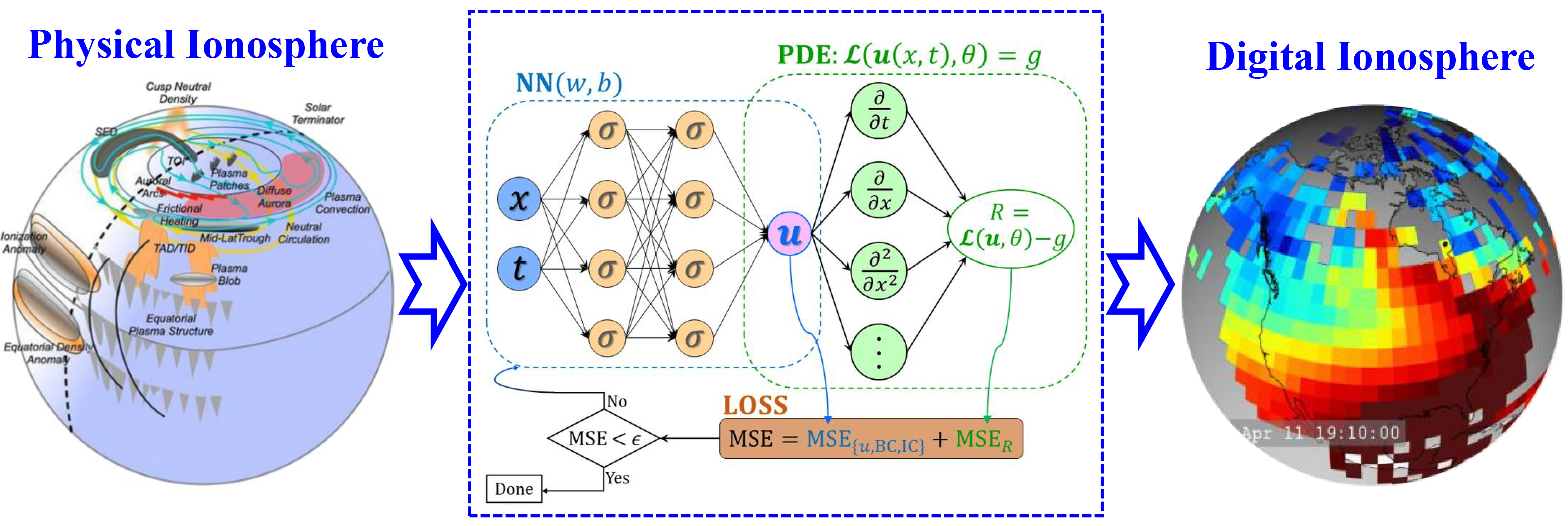
Figure 5. Ionosphere modeling and prediction with physically inspired neural network. NN: Neural network; PDE: partial differential equation; MSE: mean square error.
In ionospheric modeling, previous studies employing data assimilation and ensemble filtering techniques have been valuable approaches for integrating physical principles with real observational data[182-184]. Another promising strategy to enhance model accuracy and credibility involves combining empirical models with AI-based models. For example, integrating the IRI model with the GIM has shown potential for producing more robust global TEC products[185,186]. Both the IRI and NeQuick models[187,188], as leading empirical ionospheric models, provide essential reference data for understanding the ionosphere. When combined with precise TEC observations[189], these models offer a more detailed representation of spatio-temporal variations and transient fluctuations in the ionosphere. Rather than simply superimposing background and transient ionospheric variations, the physical principles embedded in empirical models guide the optimization of AI-based models, leading to faster computations and enhanced accuracy.
For instance, precise TEC prediction in low-latitude regions requires reliable network structures that can effectively represent and interpret complex relationships. Current DL networks often struggle to interpret causal relationships among multiple data sources, such as the coupling mechanisms between Kp (Planetary K index), Dst (Disturbance Storm Time index), and F10.7 (solar radio flux) indices and ionospheric TEC. The capability to train models with heterogeneous ionospheric data including spanning both space-borne and ground-based observations, needs further refinement. Improved training strategies are necessary to better handle joint data from multiple sources across different spatial and temporal scales. Such strategies would ultimately support more accurate long-term predictions of ionospheric variations and more effective detection and extraction of short-term anomalies.
3.7 Applications of precise ionosphere modeling and prediction
Several core applications of ionospheric modeling and prediction can be identified. (1) Positioning error correction for single-frequency GNSS receivers. Single-frequency GNSS receivers with low cost, accounting for more than 80% of the market, cannot eliminate ionospheric delay through dual frequency, and the positioning error accounts for more than 60% of ionospheric delay. With a near-real TEC map interpolation correction, the receiver can calculate ionosphere delay correction at its position point, which helps improve positioning accuracy in consumer-level GNSS applications[190,191]. (2) Rapid PPP convergence. Precise Point Positioning (PPP) technology requires a convergence time of more than 30 min, among which ionospheric delay decoupling is the bottleneck, since the traditional method relies on long observation to estimate residual error. The TEC value predicted by DL is added as prior information to PPP filter, such as virtual observation value of Kalman filter, to constrain the estimation of
ionosphere parameters. The convergence time is shortened by more than 50%, which meets the real-time and high-precision requirements of geological disaster monitoring and precision agriculture[192,193]; (3) GNSS integrity monitoring and alerting. Ionosphere disturbances pose a threat to aviation navigation. With rapid prediction of TEC variations, spatial and temporal ionospheric integrity risk maps can be generated and incorporated into satellite-based augmentation systems. High-resolution ionosphere TEC map prediction can efficiently reduce the integrity risk for civil aviation navigation systems, and further increase the GNSS augmentation availability during space weather events[194-196]. (4) Signal combination and optimization for multi-constellation and multi-frequency systems. Currently, frequency differences among GPS, GLONASS, Galileo and BDS multi-systems complicate the ionospheric delay correction. High-accuracy ionosphere map directly provides vertical TEC regardless of GNSS signal frequencies, serving as a consistent reference for multi-frequency GNSS systems. This can help improve the accuracy of multi-constellation interoperability positioning by 20%-30%, and especially enhance the availability of BDS in low latitudes[197].
The primary applications of precise ionospheric modeling and prediction span several key areas, including ionospheric delay correction for satellite navigation, precise positioning, and satellite navigation augmentation. In the context of ionospheric delay correction, well-established models such as the Klobuchar model used in the U.S. GPS system, the NeQuick model, and NTCM corrections adopted by the European GALILEO satellite navigation system, as well as the new single-frequency ionospheric correction model proposed by BDS system, have been widely implemented[198-204]. These models have been enhanced to better estimate mesoscale structures and to capture the evolving trends in the ionosphere. Additionally, the impacts of space weather on ionospheric navigation errors are effectively addressed within these models.
Another critical application of precise ionospheric modeling and prediction is assessing the impact of space weather on the middle and upper atmosphere. Previous studies have demonstrated that space weather events trigger a clear macroscopic causal chain. The explosive activity on the Sun influences Earth’s space environment through a series of processes that involve complex coupling between the magnetosphere and ionosphere. At a macroscopic level, the multiscale responses of ionospheric space weather reflect the propagation of high-speed solar wind energy through the middle and upper atmosphere. At the microscopic level, understanding the interaction among ions, electrons, and neutral particles in the ionosphere during space weather events is crucial to grasping the underlying mechanisms of ionospheric space physics. Consequently, a major challenge in ionospheric modeling today is accurately predicting and simulating the medium- and small-scale responses, as well as the evolutionary processes of ionospheric gradients, anomalies, and irregularities induced by space weather events.
4. SUMMARY AND CONCLUSIONS
This work provides a comprehensive exploration of AI-based ionospheric modeling frameworks and their typical applications. Various DL networks have been employed for spatiotemporal prediction, data completion, and feature extraction in ionospheric studies. The performance of these networks was discussed, demonstrating significant advantages over traditional ionospheric data processing methods, highlighting the considerable potential of DL techniques in advancing ionospheric research. As generative DL networks continue to develop, ionospheric modeling is expected to increasingly integrate physics-based information, empirical models, and AI methodologies.
Accurate ionospheric modeling has far-reaching implications, particularly in global and regional satellite navigation, ionospheric delay correction, and precise positioning. Furthermore, it plays a crucial role in uncovering new phenomena, mechanisms, and evolutionary patterns within ionospheric space physics.
DECLARATIONS
Authors’ contributions
Conceptualization: Liu, Y.
Methodology: Liu, Y.; Yang, K.
Writing - original draft preparation: Liu, Y.; Yang, K.
Writing - review and editing: Liu, Y.; Sun, L.; Wang, J.; Smirnov, A.; Xiong, C.
Visualization: Liu, Y.; Yang, K.
All authors have read and agreed to the published version of the manuscript.
Availability of data and materials
The original contributions presented in this study are included in the article. Further inquiries can be directed to the corresponding author.
Financial support and sponsorship
This work was supported by the National Natural Science Foundation of China under Grant 61771030.
Conflicts of interest
Liu, Y. is an Editorial Board Member of the journal Intelligence & Robotics and the Guest Editor of the Special Issue entitled “AI for Space Information and Related Applications”. She was not involved in any stage of the editorial process, including reviewer selection, manuscript handling, or decision-making. The other authors declare that they have no conflicts of interest.
Ethical approval and consent to participate
Not applicable.
Consent for publication
Not applicable.
Copyright
© The Author(s) 2026.
REFERENCES
1. Jin, S.; Wang, Q.; Dardanelli, G. A review on Multi-GNSS for earth observation and emerging applications. Remote. Sens. 2022, 14, 3930.
2. Klobuchar, J. Ionospheric time-delay algorithm for single-frequency GPS users. IEEE. Trans. Aerosp. Electron. Syst. 1987, AES-23, 325-31.
3. Davies, K.; Hartmann, G. K. Studying the ionosphere with the Global Positioning System. Radio. Sci. 1997, 32, 1695-703.
5. Coster, A.; Komjathy, A. Space weather and the global positioning system. Space. Weather. 2008, 6, 2008SW000400.
6. Akmaev, R. A. Whole atmosphere modeling: connecting terrestrial and space weather. Rev. Geophys. 2011, 49, 2011RG000364.
7. Kauristie, K.; Andries, J.; Beck, P.; et al. Space weather services for civil aviation - challenges and solutions. Remote. Sens. 2021, 13, 3685.
8. Chou, M. Y.; Lin, C. C. H.; Yue, J.; et al. Concentric traveling ionosphere disturbances triggered by Super Typhoon Meranti (2016). Geophys. Res. Lett. 2017, 44, 1219-26.
9. Savastano, G.; Komjathy, A.; Verkhoglyadova, O.; et al. Real-time detection of tsunami ionospheric disturbances with a stand-alone GNSS receiver: a preliminary feasibility demonstration. Sci. Rep. 2017, 7, 46607.
10. Blanc, E.; Jacobson, A. R. Observation of ionospheric disturbances following a 5-kt chemical explosion 2. Prolonged anomalies and stratifications in the lower thermosphere after shock passage. Radio. Sci. 1989, 24, 739-46.
11. Huang, C. Y.; Helmboldt, J. F.; Park, J.; Pedersen, T. R.; Willemann, R. Ionospheric detection of explosive events. Rev. Geophys. 2019, 57, 78-105.
12. Booker, H. G. A local reduction of F -region ionization due to missile transit. J. Geophys. Res. 1961, 66, 1073-9.
13. Mendillo, M.; Hawkins, G. S.; Klobuchar, J. A. A sudden vanishing of the ionospheric F region due to the launch of Skylab. J. Geophys. Res. 1975, 80, 2217-28.
14. Savastano, G.; Komjathy, A.; Shume, E.; et al. Advantages of geostationary satellites for ionospheric anomaly studies: ionospheric plasma depletion following a rocket launch. Remote. Sens. 2019, 11, 1734.
15. Rasheed, R.; Chen, B.; Wu, D.; Wu, L. A comparative study on multi-parameter ionospheric disturbances associated with the 2015 Mw 7.5 and 2023 Mw 6.3 earthquakes in Afghanistan. Remote. Sens. 2024, 16, 1839.
16. Akhoondzadeh, M.; De, Santis. A.; Marchetti, D.; Wang, T. Developing a deep learning-based detector of magnetic, Ne, Te and TEC anomalies from swarm satellites: The Case of Mw 7.1 2021 Japan earthquake. Remote. Sens. 2022, 14, 1582.
17. Jin, S.; Occhipinti, G.; Jin, R. GNSS ionospheric seismology: Recent observation evidences and characteristics. Earth-Sci. Rev. 2015, 147, 54-64.
18. Astafyeva, E.; Shults, K. Ionospheric GNSS imagery of seismic source: possibilities, difficulties, and challenges. J. Geophys. Res. Space. Phys. 2019, 124, 534-43.
20. Scherliess, L.; Schunk, R. W.; Sojka, J. J.; Thompson, D. C. Development of a physics-based reduced state Kalman filter for the ionosphere. Radio. Sci. 2004, 39, 2002RS002797.
21. Immel, T. J.; Harding, B. J.; Heelis, R. A.; et al. Regulation of ionospheric plasma velocities by thermospheric winds. Nat. Geosci. 2021, 14, 893-8.
22. Pasko, V. P.; Stanley, M. A.; Mathews, J. D.; Inan, U. S.; Wood, T. G. Electrical discharge from a thundercloud top to the lower ionosphere. Nature 2002, 416, 152-4.
23. Lu, G.; Richmond, A. D.; Emery, B. A.; Roble, R. G. Magnetosphere-ionosphere-thermosphere coupling: Effect of neutral winds on energy transfer and field-aligned current. J. Geophys. Res. 1995, 100, 19643-59.
24. Basu, S.; Kudeki, E.; Basu, S.; et al. Scintillations, plasma drifts, and neutral winds in the equatorial ionosphere after sunset. J. Geophys. Res. 1996, 101, 26795-809.
25. Ridley, A. J.; Richmond, A. D.; Gombosi, T. I.; De, Zeeuw. D. L.; Clauer, C. R. Ionospheric control of the magnetospheric configuration: thermospheric neutral winds. J. Geophys. Res. 2003, 108, 2002JA009464.
26. Belehaki, A.; Stanislawska, I.; Lilensten, J. An overview of ionosphere - thermosphere models available for space weather purposes. Space. Sci. Rev. 2009, 147, 271-313.
27. Rees, D.; Fuller-rowell, T. Understanding the transport of atomic oxygen within the thermosphere, using a numerical global thermospheric model. Planet. Space. Sci. 1988, 36, 935-48.
28. Roble, R. G.; Ridley, E. C.; Richmond, A. D.; Dickinson, R. E. A coupled thermosphere/ionosphere general circulation model. Geophys. Res. Lett. 1988, 15, 1325-8.
29. Richmond, A. D.; Ridley, E. C.; Roble, R. G. A thermosphere/ionosphere general circulation model with coupled electrodynamics. Geophys. Res. Lett. 1992, 19, 601-4.
30. Ridley, A.; Deng, Y.; Tóth, G. The global ionosphere-thermosphere model. J. Atmos. Sol-Terr. Phys. 2006, 68, 839-64.
31. Bilitza, D.; Altadill, D.; Truhlik, V.; et al. International reference ionosphere 2016: from ionospheric climate to real-time weather predictions. Space. Weather. 2017, 15, 418-29.
32. Pignalberi, A.; Pietrella, M.; Pezzopane, M. Towards a real-time description of the ionosphere: a comparison between international reference ionosphere (IRI) and IRI real-time assimilative mapping (IRTAM) models. Atmosphere 2021, 12, 1003.
33. Bilitza, D.; Xiong, C. A solar activity correction term for the IRI topside electron density model. Adv. Space. Res. 2021, 68, 2124-37.
34. Pignalberi, A.; Pezzopane, M.; Rizzi, R.; Galkin, I. Effective solar indices for ionospheric modeling: a review and a proposal for a real-time regional IRI. Surv. Geophys. 2018, 39, 125-67.
35. He, R.; Li, M.; Zhang, Q.; Zhao, Q. A comparison of a GNSS-GIM and the IRI-2020 model over China under different ionospheric conditions. Space. Weather. 2023, 21, e2023SW003646.
36. Radicella, S.; Leitinger, R. The evolution of the DGR approach to model electron density profiles. Adv. Space. Res. 2001, 27, 35-40.
37. Hochegger, G.; Nava, B.; Radicella, S.; Leitinger, R. A family of ionospheric models for different uses. Phys. Chem. Earth. C. 2000, 25, 307-10.
38. Wang, N.; Yuan, Y.; Li, Z.; Li, Y.; Huo, X.; Li, M. An examination of the Galileo NeQuick model: comparison with GPS and JASON TEC. GPS. Solut. 2017, 21, 605-15.
39. Kashcheyev, A.; Nava, B. Validation of NeQuick 2 model topside ionosphere and plasmasphere electron content using COSMIC POD TEC. J. Geophys. Res. Space. Phys. 2019, 124, 9525-36.
40. Feng, J.; Zhang, T.; Li, W.; Zhao, Z.; Han, B.; Wang, K. A new global TEC empirical model based on fusing multi-source data. GPS. Solut. 2023, 27, 1355.
41. Nava, B.; Coïsson, P.; Radicella, S. A new version of the NeQuick ionosphere electron density model. J. Atmos. Sol-Terr. Phys. 2008, 70, 1856-62.
42. Kelley, M. C.; Carlson, C. W. Observations of intense velocity shear and associated electrostatic waves near an auroral arc. J. Geophys. Res. 1977, 82, 2343-8.
43. Yue, X.; Schreiner, W. S.; Kuo, Y. Evaluating the effect of the global ionospheric map on aiding retrieval of radio occultation electron density profiles. GPS. Solut. 2013, 17, 327-35.
44. Radicella, S. M. New ways to modelling and predicting ionosphere variables. Atmosphere 2023, 14, 1788.
45. M. Decision tree, bagging and random forest methods detect TEC seismo-ionospheric anomalies around the time of the Chile, (Mw = 8.8) earthquake of 27 February 2010. Adv. Space. Res. 2016, 57, 2464-9.
46. Zhou, Y.; Liu, J.; Li, S.; Li, Q. Ionospheric TEC prediction based on ensemble learning models. Space. Weather. 2024, 22, e2023SW003790.
47. Han, Y.; Wang, L.; Fu, W.; Zhou, H.; Li, T.; Chen, R. Machine learning-based short-term GPS TEC forecasting during high solar activity and magnetic storm periods. IEEE. J. Sel. Top. Appl. Earth. Observations. Remote. Sensing. 2022, 15, 115-26.
48. Doven, S.; Güdar, B.; Al-nimer, K.; Aslan, Z. Estimating the effect of TEC data on rain with modelling and wavelet transformation analysis. ICCSA. 2023,. Computational. Science. and. Its. Applications. -. ICCSA. 2023. Workshops. , Gervasi, O.; Murgante, B.; Rocha, A. M .A. C.; Garau, C.; Scorza, F.; Karaca, Y.; Torre, C. M.; Eds.; Springer Nature, Cham, Switzerland, 2023; pp. 59-72.
49. Zhao, J.; Ren, B.; Wu, F.; Liu, H.; Li, G.; Li, D. TECX-TCN: Prediction of ionospheric total electron content at different latitudes in China based on XGBoost algorithm and temporal convolution network. J. Atmos. Sol-Terr. Phys. 2023, 249, 106091.
50. Nigusie, A.; Tebabal, A.; Galas, R. Modeling Ionospheric TEC using gradient boosting based and stacking machine learning techniques. Space. Weather. 2024, 22, e2023SW003821.
51. Han, Y.; Wang, L.; Chen, R.; et al. Topside ionospheric TEC modeling using multiple LEO satellites based on genetic algorithm-optimized machine learning models. GPS. Solut. 2024, 28, 1565.
52. Sivavaraprasad, G.; Lakshmi, Mallika. I.; Sivakrishna, K.; Venkata, Ratnam. D. A novel hybrid Machine learning model to forecast ionospheric TEC over low-latitude GNSS stations. Adv. Space. Res. 2022, 69, 1366-79.
53. Ji, G.; Jin, R.; Zhen, W.; Yang, H. Automatic GNSS Ionospheric scintillation detection with radio occultation data using machine learning algorithm. Appl. Sci. 2024, 14, 97.
54. Bals, A.; Thakrar, C.; Deshpande, K. B. Creating a Database to Identify high-latitude scintillation signatures with unsupervised machine learning. IEEE. J. Radio. Freq. Identif. 2022, 6, 240-9.
55. Zewdie, G. K.; Valladares, C.; Cohen, M. B.; Lary, D. J.; Ramani, D.; Tsidu, G. M. Data-driven forecasting of low-latitude ionospheric total electron content using the random forest and LSTM machine learning methods. Space. Weather. 2021, 19, e2020SW002639.
56. Zhukov, A.; Sidorov, D.; Mylnikova, A.; et al. Machine learning methodology for ionosphere total electron content nowcasting. Int. J. Artif. Intell. 2018, 16, 144-57.
57. Mcgranaghan, R. M.; Mannucci, A. J.; Wilson, B.; Mattmann, C. A.; Chadwick, R. New capabilities for prediction of high-latitude ionospheric scintillation: a novel approach with machine learning. Space. Weather. 2018, 16, 1817-46.
58. Liu, L.; Wan, W.; Chen, Y.; Le, H. Solar activity effects of the ionosphere: a brief review. Chin. Sci. Bull. 2011, 56, 1202-11.
59. Hernández-pajares, M.; Juan, J. M.; Sanz, J.; et al. The ionosphere: effects, GPS modeling and the benefits for space geodetic techniques. J. Geod. 2011, 85, 887-907.
60. Xue, D.; Wu, L.; Xu, T.; Wu, C.; Wang, Z.; He, Z. Space weather effects on transportation systems: a review of current understanding and future outlook. Space. Weather. 2024, 22, e2024SW004055.
61. Liu, L.; Wan, W.; Ning, B.; Pirog, O. M.; Kurkin, V. I. Solar activity variations of the ionospheric peak electron density. J. Geophys. Res. 2006, 111, 2006JA011598.
62. Liu, L.; Chen, Y.; Le, H.; et al. The ionosphere under extremely prolonged low solar activity. J. Geophys. Res. Space. Phys. 2011, 116, A04320.
63. Qian, L.; Burns, A. G.; Solomon, S. C. Annual/semiannual variation of the ionosphere. Geophys. Res. Lett. 2013, 40, 1928-33.
64. Zhao, B.; Wan, W.; Liu, L.; et al. Features of annual and semiannual variations derived from the global ionospheric maps of total electron content. Ann. Geophys. 2007, 25, 2513-27.
65. Azpilicueta, F.; Nava, B. A different view of the ionospheric winter anomaly. Adv. Space. Res. 2021, 67, 150-62.
66. Yasyukevich, Y. V.; Yasyukevich, A. S.; Ratovsky, K. G.; Klimenko, M. V.; Klimenko, V. V.; Chirik, N. V. Winter anomaly in NmF2 and TEC: when and where it can occur. J. Space. Weather. Space. Clim. 2018, 8, A45.
67. Shapley, A. H.; Beynon, W. J. G. ‘Winter Anomaly’ in ionospheric absorption and stratospheric warmings. Nature 1965, 206, 1242-3.
68. Hernández-Pajares, M.; Juan, J. M.; Sanz, J. Medium-scale traveling ionospheric disturbances affecting GPS measurements: Spatial and temporal analysis. J. Geophys. Res. 2006, 111, 2005JA011474.
69. Afraimovich, E. L.; Kosogorov, E. A.; Leonovich, L. A. The use of the international GPS network as the global detector (GLOBDET) simultaneously observing sudden ionospheric disturbances. Earth. Planet. Sp. 2000, 52, 1077-82.
70. Chernogor, L. F.; Mylovanov, Y. B.; Zhdanko, Y. H. Response of total electron content to the October 25, 2022 partial solar eclipse from high to low latitudes in the Euro-Asian region. Adv. Space. Res. 2024, 74, 1793-809.
71. N.; Liu, L. B.; Le, H. J. A brief review of equatorial ionization anomaly and ionospheric irregularities. Earth. Planet. Phys. 2018, 2, 257-75.
72. Eastes, R. W.; Solomon, S. C.; Daniell, R. E.; et al. Global-scale observations of the equatorial ionization anomaly. Geophys. Res. Lett. 2019, 46, 9318-26.
74. Ding, F.; Wan, W.; Xu, G.; Yu, T.; Yang, G.; Wang, J. Climatology of medium-scale traveling ionospheric disturbances observed by a GPS network in central China. J. Geophys. Res. 2011, 116, A09327.
76. Kintner, P. M.; Ledvina, B. M.; de, Paula. E. R. GPS and ionospheric scintillations. Space. Weather. 2007, 5, 2006SW000260.
78. Liu, J.; Wang, W.; Burns, A. G.; et al. In Upper Atmosphere Dynamics and Energetics; Structured storm-time polar ionosphere and its drivers: a review. American Geophysical Union and John Wiley & Sons, 2021;pp 239-52.
79. Wang, X.; Aa, E.; Chen, Y.; et al. Midlatitude neutral wind response during the Mother’s day super-intense geomagnetic storm in 2024 using observations from the Chinese meridian project. J. Geophys. Res. Space. Phys. 2025, 130, e2024JA033574.
80. Kelley, M. C.; Vlasov, M. N.; Foster, J. C.; Coster, A. J. A quantitative explanation for the phenomenon known as storm-enhanced density. Geophys. Res. Lett. 2004, 31, 2004GL020875.
81. Zhang, Q.; Moen, J.; Lockwood, M.; et al. Polar cap patch transportation beyond the classic scenario. J. Geophys. Res. Space. Phys. 2016, 121, 9063-74.
82. Wang, H.; Lühr, H.; Ma, S. Y. The relation between subauroral polarization streams, westward ion fluxes, and zonal wind: Seasonal and hemispheric variations. J. Geophys. Res. 2012, 117, 2011JA017378.
83. Zong, Q.; Reinisch, B. W.; Song, P.; Wei, Y.; Galkin, I. A. Dayside ionospheric response to the intense interplanetary shocks-solar wind discontinuities: observations from the digisonde global ionospheric radio observatory. J. Geophys. Res. 2010, 115, 2009JA014796.
84. Galkin, I. A.; Reinisch, B. W.; Huang, X.; Bilitza, D. Assimilation of GIRO data into a real-time IRI. Radio. Sci. 2012, 47, 2011RS004952.
85. Galkin, I.; Froń, A.; Reinisch, B.; et al. Global monitoring of ionospheric weather by GIRO and GNSS data fusion. Atmosphere 2022, 13, 371.
86. Reinisch, B. W.; Galkin, I. A. Global ionospheric radio observatory (GIRO). Earth. Planets. Space. 2011, 63, 377-81.
87. Estey, L. H.; Meertens, C. M. TEQC: The Multi-Purpose Toolkit for GPS/GLONASS Data. GPS. Solutions. 1999, 3, 42-9.
88. Galas, R.; Köhler, W. A binary exchange format for GPS data. Phys. Chem. Earth. A. 2001, 26, 645-8.
90. Ciraolo, L.; Azpilicueta, F.; Brunini, C.; Meza, A.; Radicella, S. M. Calibration errors on experimental slant total electron content (TEC) determined with GPS. J. Geod. 2007, 81, 111-20.
91. Ma, G.; Maruyama, T. Derivation of TEC and estimation of instrumental biases from GEONET in Japan. Ann. Geophys. 2003, 21, 2083-93.
92. Feltens, J. The activities of the Ionosphere Working Group of the International GPS Service (IGS). GPS. Solut. 2003, 7, 41-6.
93. Wielgosz, P.; Milanowska, B.; Krypiak-gregorczyk, A.; Jarmołowski, W. Validation of GNSS-derived global ionosphere maps for different solar activity levels: case studies for years 2014 and 2018. GPS. Solut. 2021, 25, 1142.
94. Jerez, G. O.; Hernández-Pajares, M.; Prol, F. S.; et al. Assessment of global ionospheric maps performance by means of ionosonde data. Remote. Sens. 2020, 12, 3452.
96. Hernández-pajares, M.; Lyu, H.; Aragón-àngel, À.; et al. Polar electron content from GPS data-based global ionospheric maps: assessment, case studies, and climatology. J. Geophys. Res. Space. Phys. 2020, 125, e2019JA027677.
97. Liu, Q.; Hernández-pajares, M.; Lyu, H.; Goss, A. Influence of temporal resolution on the performance of global ionospheric maps. J. Geod. 2021, 95, 1483.
98. Yasyukevich, Y. V.; Kiselev, A. V.; Zhivetiev, I. V.; et al. SIMuRG: system for ionosphere monitoring and research from GNSS. GPS. Solut. 2020, 24, 983.
99. Choi, J.; Lin, C. C.; Rajesh, P. K.; et al. Giant ionospheric density hole near the 2022 Hunga-Tonga volcanic eruption: multi-point satellite observations. Earth. Planets. Space. 2023, 75, 1933.
100. Astafyeva, E.; Maletckii, B.; Mikesell, T. D.; et al. The 15 January 2022 Hunga Tonga eruption history as inferred from ionospheric observations. Geophys. Res. Lett. 2022, 49, e2022GL098827.
101. Ghent, J. N.; Crowell, B. W. Spectral characteristics of ionospheric disturbances over the Southwestern Pacific from the 15 January 2022 Tonga eruption and tsunami. Geophys. Res. Lett. 2022, 49, e2022GL100145.
102. Hong, J.; Kil, H.; Lee, W. K.; Kwak, Y.; Choi, B.; Paxton, L. J. Detection of different properties of ionospheric perturbations in the vicinity of the Korean Peninsula after the Hunga-Tonga volcanic eruption on 15 January 2022. Geophys. Res. Lett. 2022, 49, e2022GL099163.
103. Le, G.; Liu, G.; Yizengaw, E.; Englert, C. R. Intense equatorial electrojet and counter electrojet caused by the 15 January 2022 Tonga volcanic eruption: space- and ground-based observations. Geophys. Res. Lett. 2022, 49, e2022GL099002.
104. Tang, L.; Li, Z.; Zhou, B. Large-area tsunami signatures in ionosphere observed by GPS TEC after the 2011 Tohoku earthquake. GPS. Solut. 2018, 22, 759.
105. Jayachandran, P. T.; Langley, R. B.; Macdougall, J. W.; et al. Canadian high arctic ionospheric network (CHAIN). Radio. Sci. 2009, 44, 2008RS004046.
106. Pereira VA, de Oliveira Camargo P. Brazilian active GNSS networks as systems for monitoring the ionosphere. GPS. Solut. 2017, 21, 1013-25.
107. Pashintsev, V. P.; Peskov, M. V.; Senokosov, M. A.; Mikhailov, D. A.; Skorik, A. D. A system for measuring the scintillation index based on the results of monitoring of small-scale fluctuations in the total electron content of the ionosphere. GPS. Solut. 2024, 28, 1550.
108. Niu, Z. Contemporary velocity field of crustal movement of Chinese mainland from Global Positioning System measurements. Chin. Sci. Bull. 2005, 50, 939-41.
109. Pignalberi, A.; Bilitza, D.; Coïsson, P.; et al. Validation of the IRI-2020 topside ionosphere options through in-situ electron density observations by low-Earth-orbit satellites. Adv. Space. Res. 2025, 75, 4192-216.
110. Smirnov, A.; Shprits, Y.; Zhelavskaya, I.; et al. Intercalibration of the plasma density measurements in earth’s topside ionosphere. J. Geophys. Res. Space. Phys. 2021, 126, e2021JA029334.
111. Smirnov, A.; Shprits, Y.; Prol, F. A novel neural network model of Earth’s topside ionosphere. Sci. Rep. 2023, 13, 1303.
112. Lin, C. H.; Wang, W.; Hagan, M. E.; et al. Plausible effect of atmospheric tides on the equatorial ionosphere observed by the FORMOSAT-3/COSMIC: three-dimensional electron density structures. Geophys. Res. Lett. 2007, 34, 2007GL029265.
113. Lin, C. Y.; Matsuo, T.; Liu, J. Y.; et al. Data assimilation of ground-based GPS and radio occultation total electron content for global ionospheric specification. J. Geophys. Res. Space. Phys. 2017, 122.
114. Zhao, B.; Wan, W.; Yue, X.; et al. Global characteristics of occurrence of an additional layer in the ionosphere observed by COSMIC/FORMOSAT-3. Geophys. Res. Lett. 2011, 38.
115. Pedatella, N. M.; Yue, X.; Schreiner, W. S. An improved inversion for FORMOSAT-3/COSMIC ionosphere electron density profiles. J. Geophys. Res. Space. Phys. 2015, 120, 8942-53.
116. Yue, X.; Schreiner, W. S.; Pedatella, N.; et al. Space weather observations by GNSS radio occultation: from FORMOSAT-3/COSMIC to FORMOSAT-7/COSMIC-2. Space. Weather. 2014, 12, 616-21.
117. Lin, C.; Lin, C. C.; Liu, J.; et al. The early results and validation of FORMOSAT-7/COSMIC-2 space weather products: global ionospheric specification and ne-aided abel electron density profile. J. Geophys. Res. Space. Phys. 2020, 125, e2020JA028028.
118. Pedatella, N. M.; Zakharenkova, I.; Braun, J. J.; et al. Processing and validation of FORMOSAT-7/COSMIC-2 GPS total electron content observations. Radio. Sci. 2021, 56, e2021RS007267.
119. La Beaujardière O. C/NOFS: a mission to forecast scintillations. J. Atmos. Sol-Terr. Phys. 2004, 66, 1573-91.
120. Jin, Y.; Spicher, A.; Xiong, C.; et al. Ionospheric plasma irregularities characterized by the swarm satellites: statistics at high latitudes. J. Geophys. Res. Space. Phys. 2019, 124, 1262-82.
121. Isham, B.; La, Hoz. C.; Kohl, H.; Hagfors, T.; Leyser, T.; Rietveld, M. Recent EISCAT heating results using chirped ISR. J. Atmos. Terr. Phys. 1996, 58, 369-83.
122. Yue, X.; Wan, W.; Ning, B.; et al. Development of the sanya incoherent scatter radar and preliminary results. J. Geophys. Res. Space. Phys. 2022, 127, e2022JA030451.
123. Yue, X.; Wan, W.; Ning, B.; Jin, L. An active phased array radar in China. Nat. Astron. 2022, 6, 619-619.
124. Wannberg, G.; Wolf, I.; Vanhainen, L.; et al. The EISCAT Svalbard radar: a case study in modern incoherent scatter radar system design. Radio. Sci. 1997, 32, 2283-307.
125. Liu, Y.; Morton, Y. J. Automatic detection of ionospheric scintillation-like GNSS satellite oscillator anomaly using a machine-learning algorithm. Navigation 2020, 67, 651-62.
126. Yang, D.; Fang, H. A low-latitude three-dimensional ionospheric electron density model based on radio occultation data using artificial neural networks with prior knowledge. Space. Weather. 2023, 21, e2022SW003299.
127. Harper, R.; Woodman, R. Preliminary multiheight radar observations of waves and winds in the mesosphere over Jicamarca. J. Atmos. Terr. Phys. 1977, 39, 959-63.
128. Camporeale, E. The challenge of machine learning in space weather: nowcasting and forecasting. Space. Weather. 2019, 17, 1166-207.
129. Wang, Z.; Zou, S.; Sun, H.; Chen, Y. Forecast global ionospheric TEC: apply modified U-Net on VISTA TEC data set. Space. Weather. 2023, 21, e2023SW003494.
130. Sun, H.; Chen, Y.; Zou, S.; et al. Complete global total electron content map dataset based on a video imputation algorithm VISTA. Sci. Data. 2023, 10, 236.
131. Zhou, H.; Zhang, S.; Peng, J.; et al. Informer: beyond efficient transformer for long sequence time-series forecasting. Proc. AAAI. Conf. Artif. Intell. 2021, 35, 11106-15.
132. Chen, L.; Zhong, X.; Zhang, F.; et al. FuXi: a cascade machine learning forecasting system for 15-day global weather forecast. NPJ. Clim. Atmos. Sci. 2023, 6, 512.
133. Bi, C.; Ren, P.; Yin, T.; Zhang, Y.; Li, B.; Xiang, Z. An informer architecture-based ionospheric foF2 model in the middle latitude region. IEEE. Geosci. Remote. Sens. Lett. 2022, 19, 1-5.
134. Zhang, Y.; Long, M.; Chen, K.; et al. Skilful nowcasting of extreme precipitation with NowcastNet. Nature 2023, 619, 526-32.
135. Lin, M.; Zhu, X.; Tu, G.; Chen, X. Optimal transformer modeling by space embedding for ionospheric total electron content prediction. IEEE. Trans. Instrum. Meas. 2022, 71, 1-14.
136. Xia, G.; Liu, M.; Zhang, F.; Zhou, C. CAiTST: conv-attentional image time sequence transformer for ionospheric TEC maps forecast. Remote. Sens. 2022, 14, 4223.
137. Luo, H.; Gong, Y.; Chen, S.; et al. Prediction of global ionospheric total electron content (TEC) based on SAM-ConvLSTM model. Space. Weather. 2023, 21, e2023SW003707.
138. Mukesh, R.; Karthikeyan, V.; Soma, P.; Sindhu, P. Prediction of TEC using NavIC/GPS data with geostatistical method/forecasting capability comparison with other models. Astrophys. Space. Sci. 2020, 365, 3868.
139. Zhukov, A. V.; Yasyukevich, Y. V.; Bykov, A. E. GIMLi: global ionospheric total electron content model based on machine learning. GPS. Solut. 2021, 25, 1055.
140. Chen, Z.; An, B.; Liao, W.; et al. Ionospheric electron density model by electron density grid deep neural network (EDG-DNN). Atmosphere 2023, 14, 810.
142. Wu, X.; Fan, C.; Tang, J.; Cheng, Y. Forecast of global ionospheric TEC using an improved transformer model. Adv. Space. Res. 2024, 73, 4519-38.
143. Tang, J.; Xu, L.; Fan, C.; Xu, C.; Ning, Y. A short-term prediction of ionospheric TEC using the RF-Prophet model for GNSS stations in China. Adv. Space. Res. 2025, 76, 3654-69.
144. Shidler, S. A.; Rodrigues, F. S. Modeling equatorial ionospheric vertical plasma drifts using machine learning. Earth. Planets. Space. 2020, 72, 1227.
145. Nigusie, A.; Tebabal, A.; Feyissa, F. Machine learning based storm time modeling of ionospheric vertical total electron content over Ethiopia. Sci. Rep. 2024, 14, 19293.
146. Han, C.; Chong, X. R.; Ou, M.; et al. Global ionospheric slab thickness prediction model using XGBoost and ensemble learning. Space. Weather. 2026, 24, e2025SW004606.
147. Ren, X.; Yang, P.; Liu, H.; Chen, J.; Liu, W. Deep learning for global ionospheric TEC forecasting: different approaches and validation. Space. Weather. 2022, 20, e2021SW003011.
148. Xia, G.; Zhang, F.; Wang, C.; Zhou, C. ED-ConvLSTM: a novel global ionospheric total electron content medium-term forecast model. Space. Weather. 2022, 20, e2021SW002959.
149. Li, L.; Liu, H.; Le, H.; et al. ED-AttConvLSTM: An ionospheric TEC map prediction model using adaptive weighted spatiotemporal features. Space. Weather. 2024, 22, e2023SW003740.
150. Wang, H.; Liu, H.; Yuan, J.; Le, H.; Shan, W.; Li, L. MAOOA-residual-attention-BiConvLSTM: an automated deep learning framework for global TEC map prediction. Space. Weather. 2024, 22, e2024SW003954.
151. Goodfellow, I.; Pouget-Abadie, J. Generative adversarial nets. In: The Twenty-Eighth Annual Conference on Neural Information Processing Systems, Advances in Neural Information Processing Systems, Ghahramani, Z., Welling, M., Cortes, C., Lawrence, N., Weinberger, K. Q., Eds.; Neural Information Processing Systems Foundation, Inc.: Montreal, Canada, 2014; Vol. 27. https://proceedings.neurips.cc/paper_files/paper/2014/file/f033ed80deb0234979a61f95710dbe25-Paper.pdf (accessed 2026-2-10).
152. Ji, E.; Moon, Y.; Park, E. Improvement of IRI global TEC maps by deep learning based on conditional generative adversarial networks. Space. Weather. 2020, 18, e2019SW002411.
153. Chen, Z.; Jin, M.; Deng, Y.; et al. Improvement of a deep learning algorithm for total electron content maps: image completion. J. Geophys. Res. Space. Phys. 2019, 124, 790-800.
154. Jeong, S.; Lee, W. K.; Jang, S.; et al. Reconstruction of the regional total electron content maps over the Korean peninsula using deep convolutional generative adversarial network and Poisson blending. Space. Weather. 2022, 20, e2022SW003131.
155. Pan, Y.; Jin, M.; Zhang, S.; Deng, Y. TEC map completion using DCGAN and Poisson blending. Space. Weather. 2020, 18, e2019SW002390.
156. Chen, J.; Fang, H.; Liu, Z. The application of a deep convolutional generative adversarial network on completing global TEC maps. J. Geophys. Res. Space. Phys. 2021, 126, e2020JA028418.
157. Pan, Y.; Jin, M.; Zhang, S.; Deng, Y. TEC map completion through a deep learning model: SNP-GAN. Space. Weather. 2021, 19, e2021SW002810.
158. Yang, K.; Liu, Y. Global Ionospheric total electron content completion with a GAN-based deep learning framework. Remote. Sens. 2022, 14, 6059.
159. Tian, P.; Yu, B.; Ye, H.; Xue, X.; Wu, J.; Chen, T. Estimation model of global ionospheric irregularities: an artificial intelligence approach. Space. Weather. 2022, 20, e2022SW003160.
160. Lan, T.; Hu, H.; Jiang, C.; Yang, G.; Zhao, Z. A comparative study of decision tree, random forest, and convolutional neural network for spread-F identification. Adv. Space. Res. 2020, 65, 2052-61.
161. Trebeschi, S.; van Griethuysen, J. J. M.; Lambregts, D. M. J.; et al. Deep learning for fully-automated localization and segmentation of rectal cancer on multiparametric MR. Sci. Rep. 2017, 7, 5301.
162. Liu, P.; Yokoyama, T.; Fu, W.; Yamamoto, M. Statistical analysis of medium-scale traveling ionospheric disturbances over Japan based on deep learning instance segmentation. Space. Weather. 2022, 20, e2022SW003151.
163. Lai, C.; Xu, J.; Lin, Z.; et al. Statistical characteristics of nighttime medium-scale traveling ionospheric disturbances from 10-years of airglow observation by the machine learning method. Space. Weather. 2023, 21, e2023SW003430.
164. Brissaud, Q.; Astafyeva, E. Near-real-time detection of co-seismic ionospheric disturbances using machine learning. Geophys. J. Int. 2022, 230, 2117-30.
165. Price, I.; Sanchez-Gonzalez, A.; Alet, F.; et al. Probabilistic weather forecasting with machine learning. Nature 2025, 637, 84-90.
166. Lam, R.; Sanchez-Gonzalez, A.; Willson, M.; et al. Learning skillful medium-range global weather forecasting. Science 2023, 382, 1416-21.
167. Bodnar, C.; Bruinsma, W. P.; Lucic, A.; et al. A foundation model for the Earth system. Nature 2025, 641, 1180-7.
168. Bi, K.; Xie, L.; Zhang, H.; Chen, X.; Gu, X.; Tian, Q. Accurate medium-range global weather forecasting with 3D neural networks. Nature 2023, 619, 533-8.
169. Sun, Y.; Liu, J.; Tsai, H.; Krankowski, A. Global ionosphere map constructed by using total electron content from ground-based GNSS receiver and FORMOSAT-3/COSMIC GPS occultation experiment. GPS. Solut. 2017, 21, 1583-91.
170. Liu, L.; Zou, S.; Yao, Y.; Wang, Z. Forecasting Global ionospheric TEC using deep learning approach. Space. Weather. 2020, 18, e2020SW002501.
171. Kaselimi, M.; Voulodimos, A.; Doulamis, N.; Doulamis, A.; Delikaraoglou, D. A causal long short-term memory sequence to sequence model for TEC prediction using GNSS observations. Remote. Sens. 2020, 12, 1354.
172. Kim, J.; Kwak, Y.; Kim, Y.; Moon, S.; Jeong, S.; Yun, J. Potential of regional ionosphere prediction using a long short-term memory deep-learning algorithm specialized for geomagnetic storm period. Space. Weather. 2021, 19, e2021SW002741.
173. Xiong, P.; Zhai, D.; Long, C.; Zhou, H.; Zhang, X.; Shen, X. Long short-term memory neural network for ionospheric total electron content forecasting over China. Space. Weather. 2021, 19, e2020SW002706.
174. Chen, J.; Zhi, N.; Liao, H.; Lu, M.; Feng, S. Global forecasting of ionospheric vertical total electron contents via ConvLSTM with spectrum analysis. GPS. Solut. 2022, 26, 1253.
175. Chen, Z.; Liao, W.; Li, H.; Wang, J.; Deng, X.; Hong, S. Prediction of global ionospheric TEC based on deep learning. Space. Weather. 2022, 20, e2021SW002854.
176. Xie, T.; Dai, Z.; Zhu, X.; Chen, B.; Ran, C. LSTM-based short-term ionospheric TEC forecast model and positioning accuracy analysis. GPS. Solut. 2023, 27, 1406.
177. Gao, X.; Yao, Y. A storm-time ionospheric TEC model with multichannel features by the spatiotemporal ConvLSTM network. J. Geod. 2023, 97, 1696.
178. Tang, J.; Zhong, Z.; Hu, J.; Wu, X. Forecasting regional ionospheric TEC maps over China using BiConvGRU deep learning. Remote. Sens. 2023, 15, 3405.
179. Ren, X.; Yang, P.; Mei, D.; Liu, H.; Xu, G.; Dong, Y. Global ionospheric TEC forecasting for geomagnetic storm time using a deep learning-based multi-model ensemble method. Space. Weather. 2023, 21, e2022SW003231.
180. Yang, D.; Fang, H.; Liu, Z. Completion of global ionospheric TEC maps using a deep learning approach. J. Geophys. Res. Space. Phys. 2022, 127, e2022JA030326.
181. Chen, Z.; Zhou, K.; Li, H.; Wang, J.; Ouyang, Z.; Deng, X. Global TEC map fusion through a hybrid deep learning model: RFGAN. Space. Weather. 2023, 21, e2022SW003341.
182. Hornik, K.; Stinchcombe, M.; White, H. Multilayer feedforward networks are universal approximators. Neural. Netw. 1989, 2, 359-66.
183. Hornik, K. Approximation capabilities of multilayer feedforward networks. Neural. Netw. 1991, 4, 251-7.
184. Schmidt-Hieber, J. The Kolmogorov-Arnold representation theorem revisited. Neural. Netw. 2021, 137, 119-26.
185. Erven T, Harremoes P. Rényi divergence and Kullback-Leibler divergence. IEEE. Trans. Inf. Theory. 2014, 60, 3797-820.
186. Menéndez, M.; Pardo, J.; Pardo, L.; Pardo, M. The Jensen-Shannon divergence. J. Frankl. Inst. 1997, 334, 307-18.
187. Shore, J.; Johnson, R. Properties of cross-entropy minimization. IEEE. Trans. Inform. Theory. 1981, 27, 472-82.
188. Alizadeh, M. M.; Schuh, H.; Todorova, S.; Schmidt, M. Global ionosphere maps of VTEC from GNSS, satellite altimetry, and formosat-3/COSMIC data. J. Geod. 2011, 85, 975-87.
189. Chen, G.; Wei, N.; Li, M.; Zhao, Q.; Zhang, J. BDS-3 and GPS/Galileo integrated PPP using broadcast ephemerides. GPS. Solut. 2022, 26, 1311.
190. Mukhtarov, P.; Pancheva, D.; Andonov, B.; Pashova, L. Global TEC maps based on GNSS data: 1. empirical background TEC model. J. Geophys. Res. Space. Phys. 2013, 118, 4594-608.
191. Mukhtarov, P.; Pancheva, D.; Andonov, B.; Pashova, L. Global TEC maps based on GNNS data: 2. model evaluation. J. Geophys. Res. Space. Phys. 2013, 118, 4609-17.
192. Prol, F. D. S.; Camargo, P. D. O.; Monico, J. F. G.; Muella, M. T. D. A. H. Assessment of a TEC calibration procedure by single-frequency PPP. GPS. Solut. 2018, 22, 701.
193. Santos Prol F, de Oliveira Camargo P, Hernandez-pajares M, de Assis Honorato Muella MT. A new method for ionospheric tomography and its assessment by ionosonde electron density, GPS TEC, and single-frequency PPP. IEEE. Trans. Geosci. Remote. Sensing. 2019, 57, 2571-82.
194. Rovira-garcia, A.; Juan, J. M.; Sanz, J.; González-casado, G.; Ibáñez, D. Accuracy of ionospheric models used in GNSS and SBAS: methodology and analysis. J. Geod. 2016, 90, 229-40.
195. Sunda, S.; Yadav, S.; Sridharan, R.; et al. SBAS-derived TEC maps: a new tool to forecast the spatial maps of maximum probable scintillation index over India. GPS. Solut. 2017, 21, 1469-78.
196. Sunda, S.; Sridharan, R.; Vyas, B. M.; et al. Satellite-based augmentation systems: A novel and cost-effective tool for ionospheric and space weather studies. Space. Weather. 2015, 13, 6-15.
197. Su, K.; Jin, S.; Hoque, M. M. Evaluation of ionospheric delay effects on multi-GNSS positioning performance. Remote. Sens. 2019, 11, 171.
198. Han, Y.; Wang, L.; Chen, R.; Fu, W.; Li, T.; Zhou, H. Toward real-time construction of global ionosphere map from ground and space-borne observations. GPS. Solut. 2022, 26, 1337.
199. Hu, T.; Xu, X.; Luo, J. Multi-source data ingestion for IRI-2020 model: a combination of ground-based and space-borne observations. GPS. Solut. 2024, 28, 1620.
200. Pedatella, N. M.; Anderson, J. L. The impact of assimilating COSMIC-2 observations of electron density in WACCMX. J. Geophys. Res. Space. Phys. 2022, 127, e2021JA029906.
201. Jakowski, N.; Hoque, M. M.; Mayer, C. A new global TEC model for estimating transionospheric radio wave propagation errors. J. Geod. 2011, 85, 965-74.
202. Hoque, M. M.; Jakowski, N. An alternative ionospheric correction model for global navigation satellite systems. J. Geod. 2015, 89, 391-406.
203. Hoque, M. M.; Jakowski, N.; Berdermann, J. Ionospheric correction using NTCM driven by GPS Klobuchar coefficients for GNSS applications. GPS. Solut. 2017, 21, 1563-72.
Cite This Article
How to Cite
Download Citation
Export Citation File:
Type of Import
Tips on Downloading Citation
Citation Manager File Format
Type of Import
Direct Import: When the Direct Import option is selected (the default state), a dialogue box will give you the option to Save or Open the downloaded citation data. Choosing Open will either launch your citation manager or give you a choice of applications with which to use the metadata. The Save option saves the file locally for later use.
Indirect Import: When the Indirect Import option is selected, the metadata is displayed and may be copied and pasted as needed.
About This Article
Special Topic
Copyright

Data & Comments
Data
0


Comments
Comments must be written in English. Spam, offensive content, impersonation, and private information will not be permitted. If any comment is reported and identified as inappropriate content by OAE staff, the comment will be removed without notice. If you have any queries or need any help, please contact us at [email protected].