


Transfer learning-based prediction of high-temperature fatigue life in Fe-based structural alloys with limited data
 0
0 Abstract
High-temperature (HT) fatigue life serves as a crucial performance metric for assessing the structural integrity and service safety of materials under elevated-temperature conditions. However, conventional assessment approaches rely on HT fatigue testing, which is typically time-consuming, costly, and experimentally challenging. Consequently, the scarcity of reliable HT fatigue data poses a major obstacle to accurate fatigue life prediction and limits the effectiveness of conventional machine learning models. In this study, a transfer learning strategy is proposed to address this data limitation by leveraging data-rich room-temperature fatigue datasets. An optimal feature subset is used with a gradient boosting decision tree model, and limited HT samples are progressively incorporated through incremental retraining to enable effective knowledge transfer across temperature domains. The results demonstrate significantly improved predictive accuracy and confirm the consistency of the dominant features across room and high temperatures. Overall, the proposed method offers a practical strategy for materials design and HT fatigue life assessment in engineering applications.
Keywords
INTRODUCTION
Fatigue failure represents a predominant concern in engineering, accounting for 80%-90% of structural fractures in mechanical components[1]. Thus, the precise assessment and prediction of the fatigue behavior of metals have substantial scientific and engineering relevance. Fatigue life refers to the number of stress cycles a material can withstand before fatigue failure under cyclic loading[2] and is influenced by multiple factors. These factors include the magnitude of the applied stress, the material’s intrinsic properties, and environmental conditions such as temperature[3-5]. While the staircase method[6] and similar tests are necessary to obtain fatigue life data, these experimental procedures are both costly and time-consuming. Furthermore, the evaluation of fatigue properties is complicated by the diversity of required test conditions, including test type, frequency, and loading parameters. These challenges are further exacerbated when fatigue behavior at elevated temperatures is considered, as high-temperature (HT) fatigue tests are particularly difficult to conduct and the corresponding experimental data are scarce[7,8].
To predict fatigue properties, a range of conventional models have been developed. These range from empirical formulations, such as the Coffin-Manson and Basquin equations[9], to physics-based approaches including the critical plane method[10], multiaxial fatigue damage models[11], energy-based methods[12], and continuum damage mechanics[13]. While valuable, these methods often rely on idealized assumptions or extensive data fitting. The complex, nonlinear interactions among factors such as manufacturing processes and service conditions are difficult to capture accurately, limiting predictive accuracy under practical uncertainties. Machine learning (ML) has recently become a powerful tool for fatigue analysis, offering superior capabilities in processing complex datasets and uncovering nonlinear patterns, enabling more accurate predictions than conventional methods[14]. It has shown promising results in predicting fatigue life[15-17], fatigue crack growth rate[18,19], and fatigue strength[20-22]. However, a significant gap remains in accurately predicting HT fatigue performance due to the scarcity of relevant data. This persistent challenge underscores the critical need for innovative approaches to achieve reliable predictions under such conditions.
As a ML paradigm, transfer learning (TL) leverages knowledge acquired from one task or domain to facilitate learning another related but distinct task or domain[23]. TL primarily aims to reduce the amount of training data required to develop a high-performing model in the target domain by leveraging pre-existing knowledge from a related source domain[24,25]. The process involves training a model on a source domain with sufficient data, then transferring and adapting this knowledge to a target domain where data acquisition is difficult. In fatigue prediction, TL has proven effective and demonstrated strong predictive performance. To enable accurate prediction of gear contact fatigue life, Li et al. proposed a TL-based strategy that leveraged data from other less expensive fatigue tests to enhance predictive performance[26]. To enable accurate prediction of the high-cycle fatigue Stress-Number of cycles (S-N) curve of steel, Wei et al. proposed a novel prediction strategy that integrates long short-term memory networks with TL, demonstrating high accuracy in predicting S-N curves across various steel types[27]. Similarly, Zhai et al. proposed a TL-enhanced physics-informed neural network that transfers knowledge of the relationship between defects and fatigue life from additive manufacturing to megacasting, enabling high-precision fatigue life predictions with limited data[28]. Despite these advances, existing TL methods still face inherent limitations when applied to cross-temperature fatigue prediction. Many of these approaches assume significant similarity in features or distributions between the source and target domains, an assumption that may not hold under drastically different thermal conditions. Moreover, most current models lack mechanisms to quantify or adapt to temperature-induced physicochemical changes explicitly, undermining the reliability of transferred knowledge. These limitations, together with the scarcity of HT data, constrain predictive accuracy and generalizability in practical HT applications, underscoring the need for novel approaches to bridge the domain gap between room and elevated temperatures effectively.
To address this problem, a TL strategy is proposed that uses room-temperature (RT) fatigue data to predict HT fatigue life. Six ML models are trained on RT fatigue data, and their performance is evaluated both with and without feature selection. Subsequently, after verifying feature consistency across temperature ranges, the optimal model and the critical feature subset are selected. The pre-trained model is then incrementally retrained on a subset of HT data to predict HT fatigue life. This work provides an effective strategy for improving fatigue life prediction under HT conditions.
MATERIALS AND METHODS
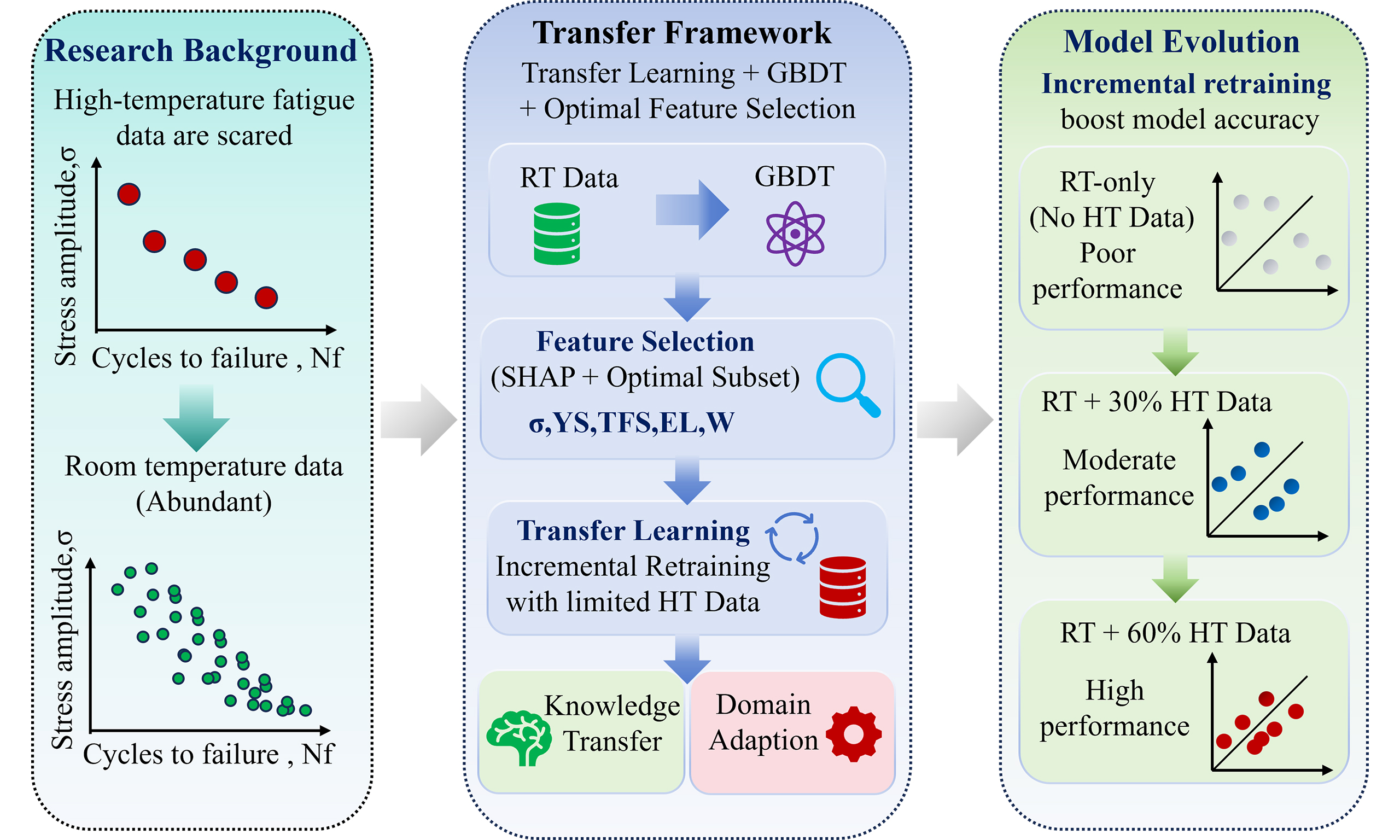
A TL strategy is proposed to address the limited availability of HT fatigue data by leveraging knowledge from extensive RT datasets, as shown in Figure 1. Initially, to establish a robust and efficient baseline, six ML models are evaluated using the full feature set from the RT data. Subsequent feature selection identified an optimal subset of five features. A comparison between the optimal feature subset and the full feature set using the same models shows no significant performance degradation, confirming that these features retain essential predictive information. The model with the highest accuracy is thus selected as the base learner. Importantly, the same optimal feature subset is identified from the HT data set, demonstrating that feature consistency across temperatures is a foundational premise for TL. Given this consistency, the TL strategy is implemented as an incremental retraining process. Specifically, the base learner is initially trained on the RT source domain using the optimal feature subset. Subsequently, HT data are progressively incorporated into the training set in increasing proportions, and the model is retrained on the combined dataset at each step. This incremental integration strategy enables the model to gradually adapt to the target domain while retaining knowledge learned from the source domain.
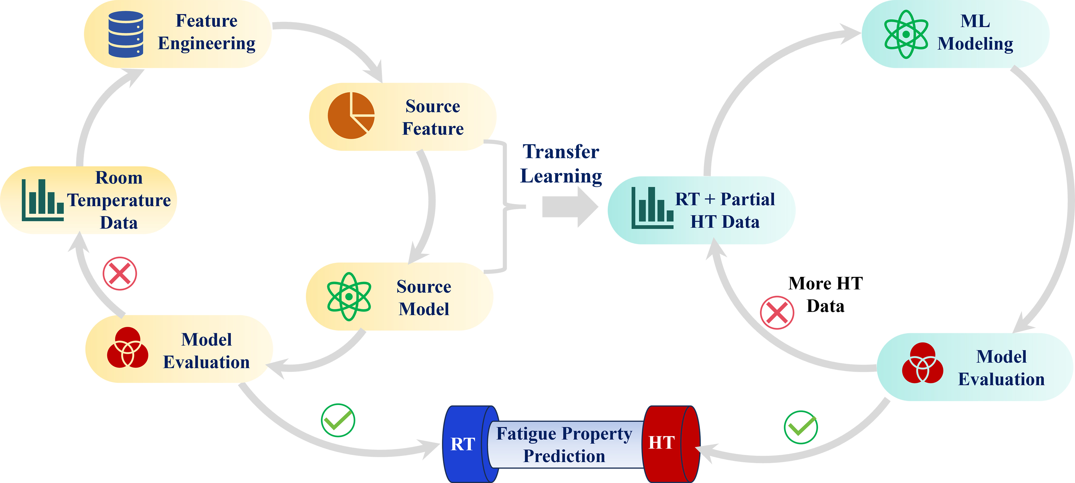
Figure 1. A TL strategy for predicting HT fatigue life using RT fatigue data. TL: Transfer learning; HT: high-temperature; RT: room-temperature; ML: machine learning.
Data collection and processing
The experimental data used in this research are obtained from the NIMS Structural Materials Data Sheet Service, a publicly available collection of fatigue data sheets published by the National Institute of Materials Science[29]. Table 1 presents data on HT and high-cycle fatigue performance for the steel grades under the specified fatigue testing conditions.
Steel grades and corresponding fatigue testing conditions employed in this research
| Steel grade | SUS403-B, S45C, SUS316-HP, SCM435, NCF800H, SUH616-B, SUS304-HP, SCMV4, ASTM A470-8 |
| Type of fatigue test | Rotating bending |
| Loading condition | Load control under zero mean stress |
| Frequency | 125 Hz |
| Stress concentration factor | 1.0 |
Given the wide dispersion of fatigue life values relative to other parameters, the data are transformed using the base-10 logarithm for analysis. After data processing, two datasets representing fatigue performance at RT and HT are formed. The RT dataset consists of 60 data points, while the HT datasets at 400, 500, and
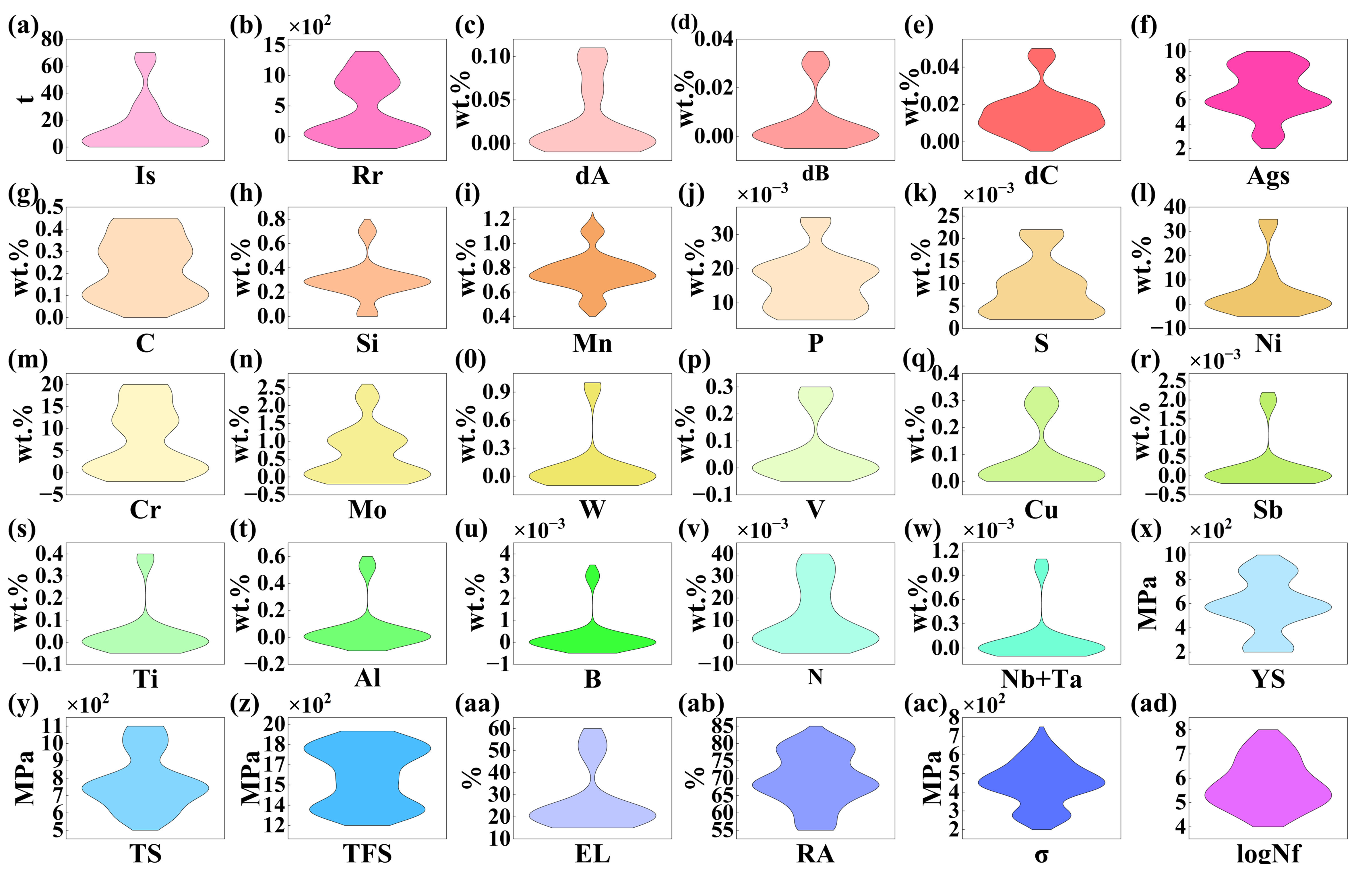
Figure 2. Overview of feature variable and target performance distributions in the dataset. Is: Ingot size; Rr: reduction ratio; dA, dB, dC: non-metallic inclusions; Ags: austenite grain size number; YS: 0.2% proof stress; TS: tensile strength; TFS: true fracture stress; EL: elongation; RA: reduction of area; σ: stress amplitude; logNf: target life.
Before performing ML, the collected data are pre-processed by normalizing each variable to the [0, 1] interval using the following equation, which eliminates the influence of differing measurement scales on model predictive performance[30].
where x is the original data value, x′ is the normalized result, min(x) and max(x) are the minimum and maximum values in the dataset, respectively.
ML algorithms
In this study, six regression algorithms, including Ridge, Lasso, random forest (RF), extreme gradient boosting (XGBoost), categorical boosting (CatBoost), and gradient boosting decision tree (GBDT), are used to model fatigue life. The six models are selected to provide a balanced comparison between interpretable linear methods and powerful nonlinear ensemble techniques. Ridge and Lasso are linear regression models with L2 and L1 regularization, respectively, that help prevent overfitting when dealing with high-dimensional features. However, their linear nature limits their ability to capture the complex nonlinear relationships common in fatigue behavior. In contrast, RF and boosting algorithms, including XGBoost, CatBoost, and GBDT, are ensemble methods that can model nonlinear interactions without requiring explicit functional forms. RF reduces overfitting by averaging predictions from multiple decision trees. XGBoost efficiently handles missing values and uses regularization to control model complexity. CatBoost is specifically designed to handle categorical features and reduce overfitting. GBDT provides a flexible framework with robust performance across various datasets. Despite their strengths, ensemble methods are generally more computationally expensive and sensitive to hyperparameter tuning[31,32].
The efficacy of these models is assessed using four key evaluation metrics, namely the coefficient of determination (R2)[33], root mean square error (RMSE)[34], mean absolute error (MAE)[35], and Pearson correlation coefficient (PCC)[36]. R2 quantifies the proportion of variance explained and serves as the primary metric for assessing a regression model’s goodness of fit, with values closer to 1 indicating greater model accuracy. MAE measures the average magnitude of errors without emphasizing large deviations, offering robustness to outliers, while RMSE calculates the square root of the mean squared error and is more sensitive to large errors. For both metrics, smaller values indicate higher predictive accuracy[37,38]. In regression problems, the PCC can be used to evaluate a model’s predictive accuracy by quantifying the linear correlation between the predicted and true values. It ranges from -1 to 1, with values close to 1 or -1 indicating a strong linear relationship and values near 0 indicating no linear correlation. These evaluation metrics are defined in Equations (2)-(5).
where yi,
To prevent overfitting while maximizing data utility, model evaluation is performed using 10-fold cross-validation[39]. This method divides the data into 10 subsets, each serving as the validation set in turn, with the remaining subsets forming the training set. This strategy is particularly beneficial for limited data, as it ensures that all data points participate in both training and validation phases, thereby enabling a thorough and reliable assessment of model performance. Each model underwent 50 independent training runs with diverse random seeds to enhance the stability and reliability of the results. The averaged R2, RMSE, MAE and PCC values are reported, with the standard deviation across repeated runs used as error bars. The hyperparameters of each model are automatically optimized using Optuna, and the corresponding parameters for all models are listed in Supplementary Table 2.
RESULTS AND DISCUSSION
Evaluation of RT models using the full dataset
The RT fatigue life is modeled using six regression algorithms with the full feature set. The evaluation metrics of these models are summarized in the radar chart shown in Figure 3A. The GBDT model demonstrates superior performance compared with the others. The scatter plot of experimental values vs. average predicted values, along with the corresponding residual plot for the GBDT model, both with error bars, is presented in Figure 3B. The GBDT model achieves the highest R2 of 0.895 (± 0.022) and PCC of 0.949 (± 0.011), and the lowest RMSE of 0.313 (± 0.030) and MAE of 0.230 (± 0.020). The model’s high accuracy in predicting fatigue life in the RT dataset is evidenced by the close alignment of most data points with the line of best fit. The residual plot shows a relatively random distribution around the zero line, with residuals predominantly confined to ± 0.5 units across the experimental range. A slight heteroscedasticity is evident, with marginally greater dispersion at higher experimental logNf values (> 6.5), indicating increased prediction uncertainty in the upper regime. The approximately symmetric scatter above and below the zero reference line corroborates the absence of significant prediction bias. The performance of the remaining models is shown in Supplementary Figure 1.
Figure 3. Performance comparison of ML models using the complete dataset, with error bars representing the standard deviation. (A) Radar chart for the performance comparison; (B) The relationship between the experimental values and the predicted values for the GBDT model, along with the corresponding residual plot (including the mean results from 50 runs with different random seeds). Test set sample size (N) = 60. Error bars represent the standard deviation of 50 independent replicates. ML: Machine learning; GBDT: gradient boosting decision tree; XGBoost: extreme gradient boosting; CatBoost: categorical boosting; RF: random forest; R2: the coefficient of determination; RMSE: root mean square error; MAE: mean absolute error; PCC: Pearson correlation coefficient; logNf: target life.
Feature engineering
Feature selection is a critical step in optimizing ML models, as it reduces complexity and computational cost by identifying and retaining only the features with the highest information content. This process not only improves model performance by mitigating overfitting but also enhances interpretability by clarifying the key factors driving predictions. Using SHapley Additive exPlanations (SHAP)[40] to rank and visualize feature importance significantly enhances the interpretability of fatigue life models. This method assigns each feature a consistent importance value based on its contribution to predictions, thereby uncovering key interactions between input variables and the target. The significance of these characteristics regarding fatigue life at RT is shown in Figure 4, and the feature importance under HT is shown in Supplementary Figure 2.
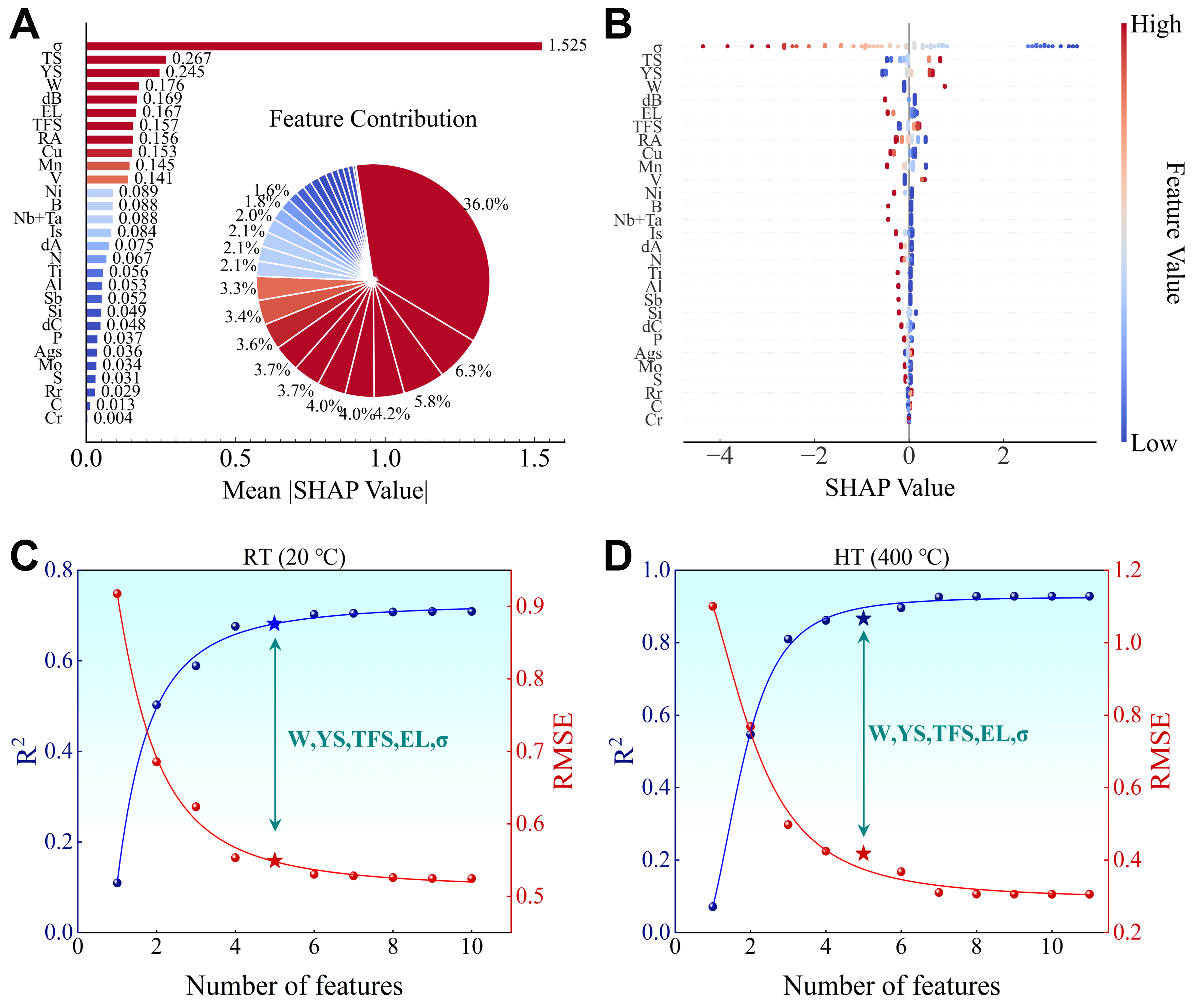
Figure 4. Further feature selection for the ML models. (A) Bar chart of feature importance and ring chart of feature contribution ratios; (B) Summary plot of SHAP values; The optimal subset selection for the (C) RT and (D) HT dataset. ML: Machine learning; SHAP: SHapley Additive exPlanations; RT: room-temperature; HT: high-temperature; σ: stress amplitude; TS: tensile strength; YS: 0.2% proof stress; dA, dB, dC: non-metallic inclusions; EL: elongation; TFS: true fracture stress; RA: reduction of area; Is: ingot size; Ags: austenite grain size number; Rr: reduction ratio; R2: the coefficient of determination; RMSE: root mean square error.
In Figure 4A and B, each point represents a SHAP value, and the color encodes the feature value according to the color bar (warmer colors indicate larger feature values, cooler colors indicate smaller feature values). When points with warmer colors cluster on the right (positive SHAP values), larger feature values tend to increase the prediction. The full ranking of feature importance guides the selection of the optimal subset. Feature importance analysis for fatigue life prediction identified σ, TS, YS, W, dB, EL, TFS, RA, Cu, and Mn as the ten most influential features, which are therefore selected for model inclusion. To further refine the feature set, the optimal subset method is applied[41]. This statistical approach evaluates all possible combinations of features to identify the subset that provides the best fit according to the specified model criteria. This method fits a least-squares model to every possible feature combination, from single features to the full feature set, and selects the best subset based on a comprehensive performance comparison.
The result of the optimal subset selection for the RT dataset is shown in Figure 4C. Due to the large number of feature subsets, only the best subsets for each subset size are shown. The analysis indicates that model performance improves with an increasing number of features, as evidenced by a rise in R2 and a corresponding decrease in RMSE. Both metrics stabilize after five features are included, suggesting that additional features contribute little to further improvement. An optimal feature subset consisting of five variables (W, YS, TFS, EL, and σ) is identified to balance predictive accuracy and model complexity. Through an exhaustive search, this subset is the optimal five‑feature combination in terms of R2 for the current dataset, and its robustness is confirmed by 10‑fold cross‑validation with 50 diverse random seeds. From a physical perspective, σ directly governs the applied stress level and is inversely correlated with fatigue life. YS and TFS reflect the material’s resistance to plastic deformation and fracture, respectively, both of which are critical under cyclic loading. EL represents ductility, which influences fatigue crack initiation and propagation. The W content can improve fatigue performance through solid solution strengthening and precipitation hardening induced by fine particles, thereby enhancing the alloy’s fatigue resistance[42]. The inclusion of these five features thus captures the key factors governing fatigue behavior while maintaining model simplicity.
Post-selection evaluation of RT models
The five features identified through feature selection in the previous section are used as inputs to the ML model. The performance of the diverse models is shown in the radar chart in Figure 5A. Compared with the case using all features, no significant degradation in model performance is observed, indicating the reasonableness of the feature engineering process. Among the six evaluated ML models, the GBDT model again demonstrated the highest prediction accuracy, achieving the highest R2 (0.893 ± 0.023) and PCC (0.948 ± 0.012), along with the lowest RMSE (0.317 ± 0.032) and MAE (0.234 ± 0.020). The scatter plot of the GBDT model showing the relationship between the experimental and predicted values, along with the corresponding residual plot, is shown in Figure 5B. The predictions are in close agreement with the experimental values, with relatively small errors. Therefore, the GBDT models developed in this study demonstrate satisfactory predictive capability and stability for fatigue life prediction within the compositional scope of the original dataset, as evidenced by R2 values exceeding 0.85 and error bars smaller than 0.03. The residuals show an approximately symmetric distribution around the zero baseline, with most data points clustered within a narrow ± 0.5 interval. A slight deviation is observed at the lower and upper ends of the dataset. The residual variance is smaller for the experimental logNf values below 4.5, whereas a larger spread with a few positive residuals is observed for the values above 7.0, indicating reduced prediction accuracy in these regions. In the central range of experimental logNf (5.5-6.8), the residuals are randomly distributed around zero with small bias. Additionally, the detailed performance of the remaining models on the RT dataset after feature selection is presented in Supplementary Figure 3.
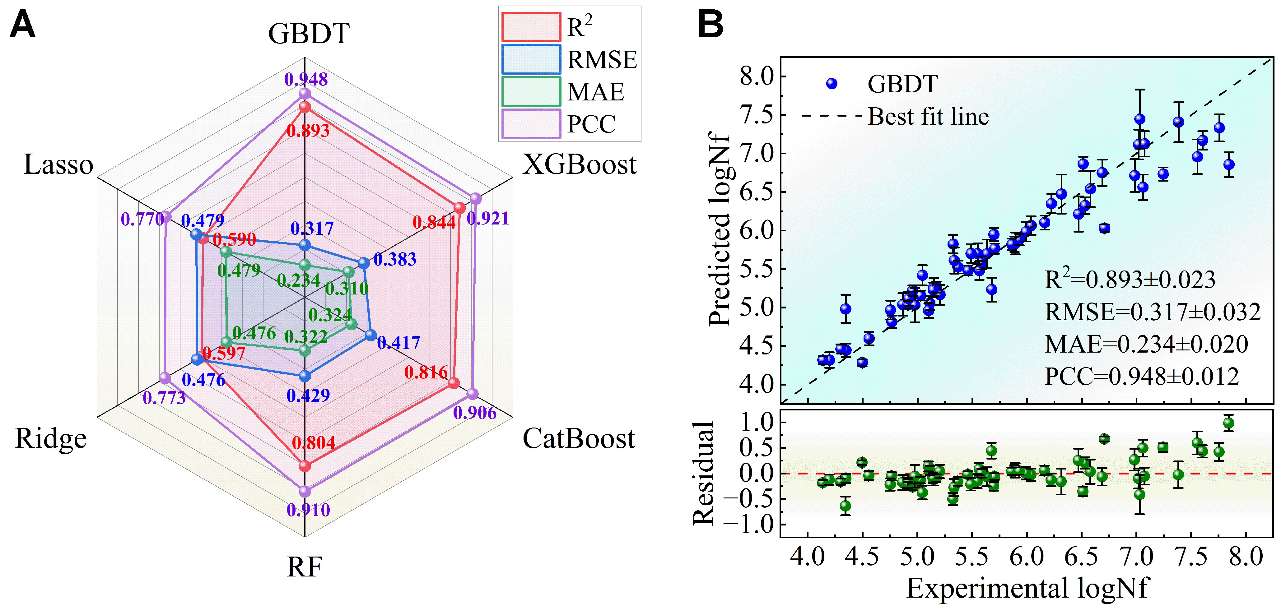
Figure 5. Comparison of model performance after feature selection, with error bars representing the standard deviation. (A) Radar chart for the performance comparison; (B) The relationship between the experimental values and the predicted values for the GBDT model, along with the corresponding residual plot (including the mean results from 50 runs with different random seeds). Test set sample size (N) = 60. Error bars represent the standard deviation of 50 independent replicates. GBDT: Gradient boosting decision tree; XGBoost: extreme gradient boosting; CatBoost: categorical boosting; RF: random forest; R2: the coefficient of determination; RMSE: root mean square error; MAE: mean absolute error; PCC: Pearson correlation coefficient; logNf: target life.
Transfer learning for HT fatigue life prediction
Directly applying the GBDT model trained on RT data to predict HT fatigue life yields poor results and shows virtually no predictive capability. This discrepancy underscores the model’s inadequacy in predicting HT behavior when trained solely on RT data. Physically, HT exposure induces substantial microstructural evolution in steels, including recovery, recrystallization, precipitate coarsening, and dislocation structure rearrangement. Consequently, fatigue resistance and failure mechanisms differ fundamentally between RT and HT conditions. Even when the chemical composition and loading conditions remain identical, the underlying physical processes governing fatigue life are not directly transferable. Statistically, the relationship between input features and fatigue life shows a domain shift from RT to HT, indicating that the feature-target distributions in the two domains are misaligned. To bridge this domain gap, the TL strategy detailed in Section “MATERIALS AND METHODS” is employed. In this strategy, RT fatigue life serves as the source domain, while HT fatigue life constitutes the target domain. To implement TL effectively, feature selection is first performed on the HT data to align feature importance with that of the RT dataset. Using the optimal subset method, the key features for HT fatigue life are identified. As illustrated in Figure 4D, the optimal feature set comprising W, YS, TFS, EL, and σ aligns closely with the feature set derived from RT data. Furthermore, feature selection was performed at elevated temperatures of 500 and 600 °C, and the results exhibited the same characteristics as those observed in the RT dataset, as shown in Supplementary Figure 4. Building on these selected features, TL is applied by training a model on RT fatigue data to predict HT fatigue life, thereby mitigating the challenge of limited HT data availability. By incrementally increasing the proportion of HT data during training, the model is continuously refined to better capture material behavior under elevated temperatures, which reduces prediction discrepancies and improves generalization across varying thermal conditions.
The performance of the GBDT model is systematically evaluated by progressively incorporating HT data into the RT training set in 10% increments, from 10% to 90%. The remaining HT data are reserved as a test set. Additionally, the efficacy of the TL strategy is verified using a dataset containing only HT data for comparison. To ensure robustness, each configuration is trained 50 times using different random seeds. As illustrated in Figure 6A, the average R2 values from both evaluation strategies increase monotonically as HT data are incorporated, indicating that the model progressively adapts to the target domain. For the HT-only model, the R2 values are 0.368 and 0.825 when 30% and 60% HT data are used, respectively. More importantly, across all HT data fractions, the model trained on the combined RT-HT dataset consistently outperforms the model trained solely on HT data, demonstrating that knowledge learned from the data-rich RT domain provides a beneficial initialization and significantly enhances predictive capability under limited HT data conditions. This result highlights the necessity of the TL strategy, particularly when HT data are scarce. The GBDT model achieves the best performance on the RT dataset and is therefore initially considered suitable for TL from RT to HT. However, this remains an assumption, so TL from RT to HT is performed for all models as shown in Supplementary Figures 5-9, and the GBDT model is ultimately selected after a comprehensive comparison of their performance.
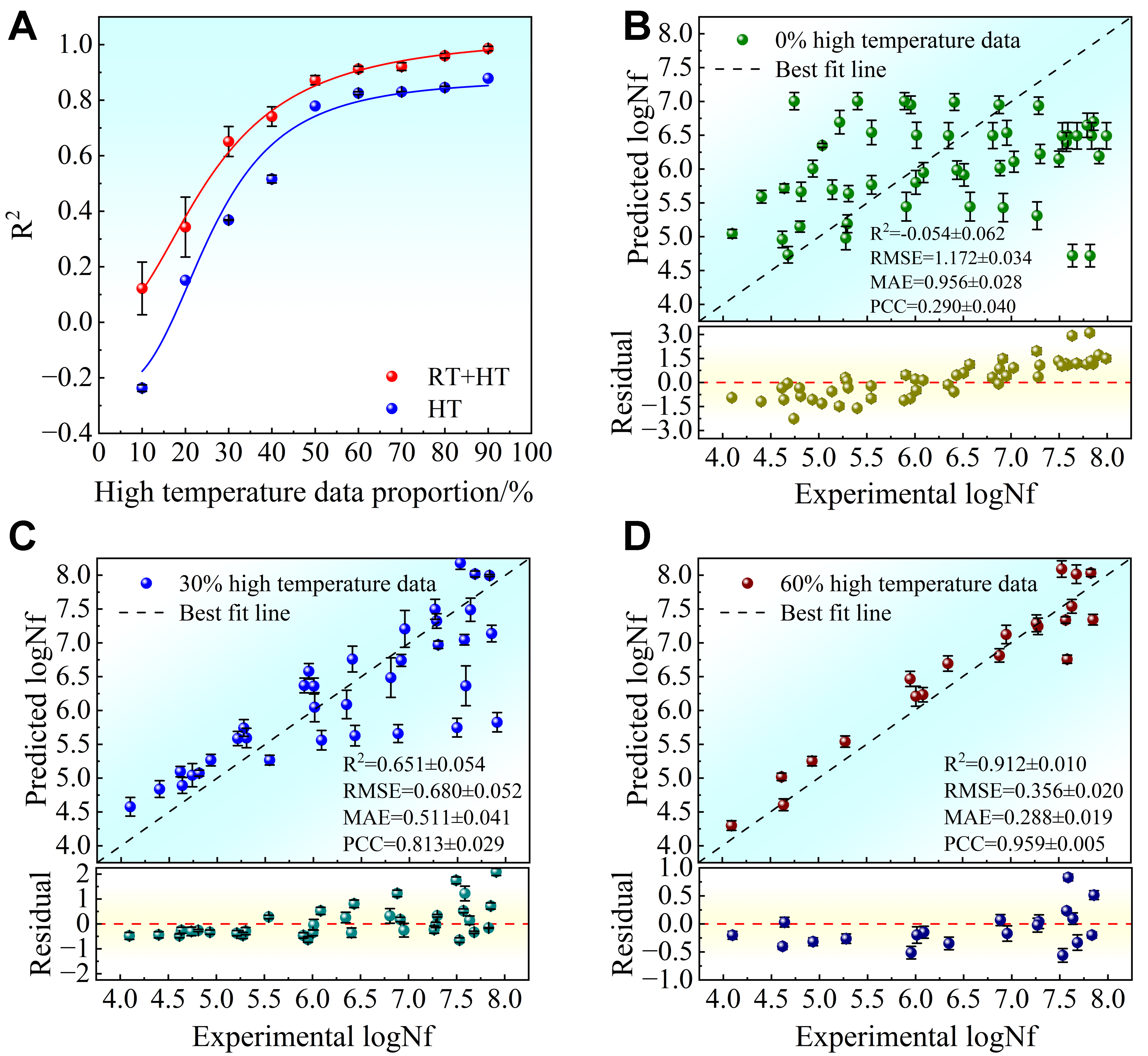
Figure 6. The influence of HT data proportion on the fatigue life prediction precision of the GBDT model, with error bars representing the standard deviation. (A) Comparison of R2 values for GBDT models trained on mixed vs. HT only data; (B-D) Prediction performance on the remaining HT test set when 0%, 30%, and 60% of HT data are incorporated into the training set, respectively. Test set sample size (N): 0% HT = 50, 30% HT = 35, 60% HT = 20. Error bars represent the standard deviation of 50 independent replicates. HT: High-temperature; GBDT: gradient boosting decision tree; R2: the coefficient of determination; RT: room-temperature; logNf: target life; RMSE: root mean square error; MAE: mean absolute error; PCC: Pearson correlation coefficient.
The averaged performance over 50 iterations for mixing ratios of 0%, 30%, and 60% HT data is shown in Figure 6B-D, respectively. When no HT data are included [Figure 6B], the model exhibits poor predictive capability, with negative R2 values, indicating a difference between the RT and HT domains. Incorporating 30% HT data yields moderate predictive accuracy (R2 = 0.651), while increasing the fraction to 60% significantly improves performance (R2 = 0.912), accompanied by substantial reductions in RMSE and MAE and a marked increase in PCC. This improvement is further corroborated by the evolution of the residual distributions. As shown in Figure 6B-D, the residuals progressively transition from systematic bias to stochastic dispersion as HT data increase. At 0% HT data, residuals show pronounced negative deviations across the entire prediction range, indicating a systematic overestimation of fatigue life. With 30% HT data, the residual distribution becomes approximately symmetric around zero, although noticeable variance and heteroscedasticity persist, particularly at higher fatigue life levels. When the HT fraction reaches 60%, residuals collapse into a narrow and homoscedastic band, indicating stable and unbiased predictions. The progressive performance improvement with increasing HT data reflects the model’s enhanced adaptation to the target domain through the incorporation of HT information. Transfer predictions are further investigated across temperatures ranging from RT to 500 °C and from RT to 600 °C, as presented in Supplementary Figures 10 and 11, respectively. These results not only confirm the effectiveness of the TL strategy but also provide empirical evidence for consistent fatigue behavior patterns across temperatures, thereby fundamentally justifying the applicability of TL in this context.
The present strategy is fundamentally data-driven and does not explicitly incorporate microstructural evolution or temperature-dependent deformation mechanisms. Although consistent feature subsets are identified across RT and HT datasets, this consistency reflects similarity in predictive relevance rather than mechanistic equivalence. The failure of direct RT-to-HT prediction indicates a significant domain gap, whereas improved performance with increasing HT data suggests that model adaptation relies on partial retraining. Therefore, the proposed approach should be understood as a TL strategy that improves data efficiency rather than a strict transfer of physical knowledge. HT fatigue involves additional mechanisms such as creep-fatigue interaction, oxidation-assisted damage, and microstructural instability, which are not explicitly captured in the present strategy due to data limitations[43]. Instead, their effects are indirectly embedded in macroscopic descriptors such as strength and elongation.
The input features include compositional, processing, and macroscopic mechanical descriptors, which are used to establish predictive relationships with fatigue life. These descriptors are treated as static, global variables and do not explicitly capture microstructural evolution or local damage processes during fatigue. Although microstructural features such as grain size and inclusion characteristics are included, their roles are represented only through statistical correlations rather than explicit mechanistic modeling. Consequently, SHAP-based feature importance reflects predictive relevance rather than causal relationships between microstructure, deformation, and fatigue damage evolution. The observed feature consistency across temperatures therefore indicates similarity in statistical patterns within the dataset, rather than invariance of the underlying physical mechanisms. Given the current data availability, macroscopic properties such as strength and elongation can be regarded as integrated surrogate descriptors that implicitly capture the combined influence of microstructure and its evolution. However, incorporating microstructure-sensitive descriptors and explicitly modeling temperature-dependent microstructure evolution remain necessary to improve physical interpretability and extrapolation capability in future work. Importantly, the proposed TL strategy is developed and validated specifically for alloy steels under the testing conditions summarized in Table 1 (rotating bending, load control with zero mean stress, 125 Hz).
CONCLUSION
In this study, comprehensive datasets describing the fatigue life of steels at both RT and HT are compiled. ML model development and feature selection are first conducted using the RT dataset to identify critical variables governing fatigue life. Subsequently, a TL strategy is implemented to enable HT fatigue life prediction by leveraging knowledge learned from RT data and incorporating a limited amount of HT data for incremental retraining. This method utilized knowledge from RT data by incorporating a limited portion of HT data into the training process, thereby significantly enhancing the prediction accuracy of the GBDT model for HT fatigue life. Using this applied methodology, the effectiveness of predicting material fatigue life across different temperatures is validated, and the consistency of material properties across various temperature ranges is confirmed via the optimal subset method. The study provides a practical strategy for material selection and design in HT applications and offers guidance for future predictive modeling of material performance under a variety of operating conditions.
DECLARATIONS
Authors’ contributions
Writing - original draft, software, methodology, formal analysis, data curation: Wang, Q.; Shang, C.
Writing - review and editing, supervision, project administration, investigation: Wu, H. H.; Zhu, D.
Validation, investigation, data collection: Wang, S.; Gao, J.
Visualization, resources, formal analysis, conceptualization: Zhao, H.; Zhang, C.; Huang, Y.
Supervision, conceptualization, revised and finalized the manuscript: Lu, J.; Mao, X.
Availability of data and materials
The dataset used in this study is obtained from the NIMS Structural Materials Data Sheet Service (available at https://fds.nims.go.jp/), specifically focusing on the “Elevated-Temperature, High-Cycle Fatigue Properties” data sheets. The processed data that support the findings of this study are available from the corresponding author upon reasonable request. Additionally, the source code and project files used in this research have been made available in the following GitHub repository: https://github.com/wq360/project.git.
AI and AI-assisted tools statement
Not applicable.
Financial support and sponsorship
This work is financially supported by the Advanced Materials-National Science and Technology Major Project: 2025ZD0619601. Wu, H. H. also thanks the financial support from the Xiaomi Young Scholars Program, and the Xiaomi Open-Competition Research Program (39990320). The computing work is supported by USTB MatCom of Beijing Advanced Innovation Center for Materials Genome Engineering.
Conflicts of interest
Wu, H. H. is a Youth Editorial Board Member of the journal Journal of Materials Informatics, and a Guest Editor of the Special Topic “Predictive Materials Informatics for Extreme Conditions”, but was not involved in any steps of editorial processing, notably including reviewer selection, manuscript handling, and decision making, while the other authors have declared that they have no conflicts of interest.
Ethical approval and consent to participate
Not applicable.
Consent for publication
Not applicable.
Copyright
© The Author(s) 2026.
Supplementary Materials
REFERENCES
1. Li, Y.; Liu, J.; Huang, W.; Zhang, S. Microstructure related analysis of tensile and fatigue properties for sand casting aluminum alloy cylinder head. Eng. Fail. Anal. 2022, 136, 106210.
3. Peng, W.; Xue, H.; Ge, R.; Peng, Z. The influential factors on very high cycle fatigue testing results. MATEC. Web. Conf. 2018, 165, 20002.
4. Yang, G.; Wang, M.; Li, Q.; Ding, R. Methodology to evaluate fatigue damage of high-speed train welded bogie frames based on on-track dynamic stress test data. Chin. J. Mech. Eng. 2019, 32, 365.
5. Jimenez-Martinez, M. Manufacturing effects on fatigue strength. Eng. Fail. Anal. 2020, 108, 104339.
6. Dixon, W. J.; Mood, A. M. A method for obtaining and analyzing sensitivity data. J. Am. Stat. Assoc. 1948, 43, 109-26.
7. Veile, G.; Rudolph, J.; Grözinger, N.; Herzig, M.; Grimm, M.; Weihe, S. Improving fatigue testing of AISI 304L stainless steel in high temperature water regarding their complex hardening and softening material behaviour. Int. J. Press. Vessel. Pip. 2025, 218, 105612.
8. Hirose, T.; Sakasegawa, H.; Nakajima, M.; Kato, T.; Miyazawa, T.; Tanigawa, H. Effects of test environment on high temperature fatigue properties of reduced activation ferritic/martensitic steel, F82H. Fusion. Eng. Des. 2018, 136, 1073-6.
9. Kamal, M.; Rahman, M. Advances in fatigue life modeling: a review. Renew. Sustain. Energy. Rev. 2018, 82, 940-9.
10. Zhu, S.; Yu, Z.; Correia, J.; De Jesus, A.; Berto, F. Evaluation and comparison of critical plane criteria for multiaxial fatigue analysis of ductile and brittle materials. Int. J. Fatigue. 2018, 112, 279-88.
11. Fatemi, A.; Socie, D. F. A critical plane approach to multiaxial fatigue damage including out‐of‐phase loading. Fatigue. Fract. Eng. Mat. Struct. 1988, 11, 149-65.
12. Wang, H.; Liu, X.; Chen, T.; Xu, S. Prediction and evaluation of fatigue life via modified energy method considering surface processing. Int. J. Damage. Mech. 2022, 31, 426-43.
13. Cui, W. A state-of-the-art review on fatigue life prediction methods for metal structures. J. Mar. Sci. Technol. 2002, 7, 43-56.
14. Shang, C.; Jiang, T.; Wu, H.; et al. Efficient design of hydrogen-resistant ultra-high-strength steels via active learning and multiscale characterization. Corros. Commun. 2026, 21, 60-72.
15. Zhang, M.; Sun, C.; Zhang, X.; et al. High cycle fatigue life prediction of laser additive manufactured stainless steel: a machine learning approach. Int. J. Fatigue. 2019, 128, 105194.
16. Yang, J.; Kang, G.; Liu, Y.; Kan, Q. A novel method of multiaxial fatigue life prediction based on deep learning. Int. J. Fatigue. 2021, 151, 106356.
17. Arvanitis, K.; Nikolakopoulos, P.; Pavlou, D.; Farmanbar, M. Machine learning-based fatigue lifetime prediction of structural steels. Alexandria. Eng. J. 2025, 125, 55-66.
18. Freed, Y. Machine learning-based predictions of crack growth rates in an aeronautical aluminum alloy. Theor. Appl. Fract. Mech. 2024, 130, 104278.
19. Rathore, S.; Kumar, A.; Kumar, A.; Mishra, K.; Singh, A. Prediction of sub-critical fatigue crack growth rate in a high-carbon tempered martensitic steel at varying R ratio: experimental investigation and machine learning based modelling. Int. J. Fatigue. 2025, 193, 108804.
20. Shiraiwa, T.; Miyazawa, Y.; Enoki, M. Prediction of fatigue strength in steels by linear regression and neural network. Mater. Trans. 2018, 60, 189-98.
21. Choi, D. Data-driven materials modeling with XGBoost algorithm and statistical inference analysis for prediction of fatigue strength of steels. Int. J. Precis. Eng. Manuf. 2019, 20, 129-38.
22. Yan, F.; Song, K.; Liu, Y.; Chen, S.; Chen, J. Predictions and mechanism analyses of the fatigue strength of steel based on machine learning. J. Mater. Sci. 2020, 55, 15334-49.
23. Pan, S. J.; Yang, Q. A survey on transfer learning. IEEE. Trans. Knowl. Data. Eng. 2010, 22, 1345-59.
24. Tang, S.; Ma, J.; Yan, Z.; Zhu, Y.; Khoo, B. C. Deep transfer learning strategy in intelligent fault diagnosis of rotating machinery. Eng. Appl. Artif. Intell. 2024, 134, 108678.
25. Hu, J.; Chen, M.; Tang, H.; Zhang, J. An adversarial transfer learning method based on domain distribution prediction for aero-engine fault diagnosis. Eng. Appl. Artif. Intell. 2024, 133, 108287.
26. Li, Y.; Wei, P.; Xiang, G.; Jia, C.; Liu, H. Gear contact fatigue life prediction based on transfer learning. Int. J. Fatigue. 2023, 173, 107686.
27. Wei, X.; Zhang, C.; Han, S.; Jia, Z.; Wang, C.; Xu, W. High cycle fatigue S-N curve prediction of steels based on transfer learning guided long short term memory network. Int. J. Fatigue. 2022, 163, 107050.
28. Zhai, Q.; Liu, Z.; Zhu, P. A transfer learning enhanced physics-informed neural network for predicting fatigue life of megacasting alloy with limited data sizes. Int. J. Fatigue. 2025, 200, 109129.
29. Furuya, Y.; Nishikawa, H.; Hirukawa, H.; Nagashima, N.; Takeuchi, E. Catalogue of NIMS fatigue data sheets. Sci. Technol. Adv. Mater. 2019, 20, 1055-72.
30. Patro, S. G. K.; Sahu, K. K. Normalization: a preprocessing stage. arXiv 2015, arXiv:1503.06462. https://doi.org/10.48550/arXiv.1503.06462. (accessed 2026-06-03).
31. Miao, B.; Lin, G.; Zhang, Y.; Cheng, Y.; Yang, H. Machine learning applications in metallic materials: recent advances and future perspectives. J. Alloys. Compd. 2026, 1062, 187486.
32. Shmuel, A.; Glickman, O.; Lazebnik, T. A comprehensive benchmark of machine and deep learning models on structured data for regression and classification. Neurocomputing 2025, 655, 131337.
33. Colin Cameron, A.; Windmeijer, F. A. An R-squared measure of goodness of fit for some common nonlinear regression models. J. Econom. 1997, 77, 329-42.
34. Herlocker, J. L.; Konstan, J. A.; Terveen, L. G.; Riedl, J. T. Evaluating collaborative filtering recommender systems. ACM. Trans. Inf. Syst. 2004, 22, 5-53.
35. Cleger-Tamayo, S.; Fernández-Luna, J. M.; Huete, J. On the use of weighted mean absolute error in recommender systems. 2012. https://api.semanticscholar.org/CorpusID:16692759. (accessed 2026-06-03).
36. Sheugh, L.; Alizadeh, S. H. A note on Pearson correlation coefficient as a metric of similarity in recommender system. In 2015 Ai & Robotics (IRANOPEN), Qazvin, Iran. Apr 12, 2015. IEEE; 2015. p. 1-6.
37. Chai, T.; Draxler, R. R. Root mean square error (RMSE) or mean absolute error (MAE)? - Arguments against avoiding RMSE in the literature. Geosci. Model. Dev. 2014, 7, 1247-50.
38. Shang, C.; Zhu, D.; Wu, H.; et al. A quantitative relation for the ductile-brittle transition temperature in pipeline steel. Scr. Mater. 2024, 244, 116023.
39. Efron, B. Estimating the error rate of a prediction rule: improvement on cross-validation. J. Am. Stat. Assoc. 1983, 78, 316-31.
40. Lundberg, S.; Lee, S. I. A unified approach to interpreting model predictions. arXiv 2017, arXiv:1705.07874. https://doi.org/10.48550/arXiv.1705.07874. (accessed 2026-06-03).
41. Kohavi, R.; John, G. H. Wrappers for feature subset selection. Artif. Intell. 1997, 97, 273-324.
42. Park, J. S.; Kim, S. J.; Lee, C. S. Effect of W addition on the low cycle fatigue behavior of high Cr ferritic steels. Mater. Sci. Eng. A. 2001, 298, 127-36.
Cite This Article
How to Cite
Download Citation
Export Citation File:
Type of Import
Tips on Downloading Citation
Citation Manager File Format
Type of Import
Direct Import: When the Direct Import option is selected (the default state), a dialogue box will give you the option to Save or Open the downloaded citation data. Choosing Open will either launch your citation manager or give you a choice of applications with which to use the metadata. The Save option saves the file locally for later use.
Indirect Import: When the Indirect Import option is selected, the metadata is displayed and may be copied and pasted as needed.
About This Article
Special Topic
Copyright

Data & Comments
Data
0


Comments
Comments must be written in English. Spam, offensive content, impersonation, and private information will not be permitted. If any comment is reported and identified as inappropriate content by OAE staff, the comment will be removed without notice. If you have any queries or need any help, please contact us at [email protected].