


Multi-fidelity learning in materials informatics: methodologies, applications, and outlook
 0
0 Abstract
Data-driven methods are transforming materials design by accelerating the discovery of new compounds and the optimization of existing systems. However, the progress of such approaches is often constrained by the scarcity of high-fidelity data from experiments and advanced simulations. Multi-fidelity (MF) learning has emerged as a powerful strategy to address this challenge by integrating information from diverse data sources that vary in accuracy and cost. In this review, we provide a systematic overview of the major methodologies for MF learning, including statistical and parametric models, machine learning models with fidelity features, correction-based models such as co-kriging, deep learning frameworks, and active learning frameworks. We discuss the strengths, limitations, and typical applications of each method in materials science, with illustrative examples spanning electronic structure modeling, alloy design, and interatomic potential development. Cross-cutting issues are also examined, including the bias-variance trade-off, data requirements for nested vs. non-nested designs, and computational scalability. Finally, we highlight outstanding challenges and outline emerging opportunities, such as physics-informed and generative MF models, standardized datasets, and integration with autonomous laboratories. Together, these perspectives define a roadmap for advancing MF learning as a core enabler of next-generation materials discovery.
Keywords
INTRODUCTION
Data-driven methodologies are increasingly being utilized to accelerate the design and discovery of new materials[1-11]. At the core of these approaches lies data, which provide the foundation for training predictive models and guiding design strategies[12-17]. Yet the accelerating pace of materials discovery is constrained by a persistent data bottleneck, where high-fidelity (HF) data are scarce while low-fidelity (LF) data are abundant[18-23]. To formalize this disparity in data quality, we introduce the notion of data fidelity. Here, “fidelity” refers to the quality of a data source or model, encompassing its systematic bias relative to the desired high-truth target, its noise level or predictive variance, and the completeness/integrity of the recorded variables. HF sources, such as density functional theory (DFT) calculations at the hybrid functional level[9,24-27] or experimental measurements of structural, electronic, and mechanical properties[28-30], are regarded as the gold standard. Although these methods provide accurate and reliable information, they are costly in terms of computational resources, experimental effort, or wall-clock time, which limits their scalability across the vast chemical and structural design space[31]. By comparison, LF data, including semi-empirical simulations, classical force fields, and simplified experiments, are much more accessible but inevitably less accurate and possibly biased[28-30,32,33]. Bridging the divide between scarce, high-quality data and plentiful, low-quality data remains a central challenge for materials informatics. This challenge has motivated the development of strategies capable of jointly leveraging information across fidelity levels.
Among these strategies, multi-fidelity (MF) learning has emerged as a powerful approach to overcome such a bottleneck. In essence, MF learning refers to a class of machine learning approaches that integrate information from datasets of varying accuracy and cost, such as combining LF simulations with HF experimental measurements[34-36]. The central idea is to exploit the complementary strengths of different data sources: LF data provide broad coverage of the design space and capture general trends in materials performance, while HF data anchor the models with reliable accuracy[28,37,38]. By learning correlations and systematic discrepancies between fidelity levels, MF approaches can effectively transfer knowledge across datasets, yielding predictions that are both accurate and data-efficient[34,39-45]. This paradigm is particularly promising for materials design, where exhaustive HF characterization is prohibitively expensive, yet the demand for predictive accuracy is high[28-30,32,33]. Key methodological ideas include statistical and parametric models, machine learning models with fidelity features, correction-based models such as co-kriging, deep learning frameworks, and active learning frameworks, each offering distinct trade-offs in terms of accuracy, scalability, and interpretability[46-50]. Together, these strategies enable the construction of surrogate models with higher accuracy and lower costs, thereby accelerating materials discovery[29,51-53].
MF learning has broad practical relevance across materials research, spanning high-throughput screening pipelines[42,54], interatomic potential predictions[38-40], and data-driven design of new materials[37,55]. In steel design, it couples fast thermo-micromechanical surrogates with strategically chosen HF finite element evaluations to optimize strain-hardening performance with both efficiency and accuracy[53]. In halide perovskites, MF machine learning integrates semi-local and hybrid-functional DFT data with experimental measurements to predict decomposition energies, guiding the genetic algorithm-driven discovery of stable photovoltaic alloys[56]. In polymers, a MF co-training neural network fuses all-atom molecular dynamics simulation data (LF) with scarce experimental measurements (HF) to accurately predict phthalonitrile melting points, enabling low-cost screening of low-melting candidates for improved processability[57]. In geomaterials, an active-learning MF residual Gaussian process (GP) framework was trained on abundant LF data collected across multiple sites, with predictive uncertainty used as an acquisition function to guide HF sampling. This approach demonstrated robust extrapolation in sparsely sampled regions and significantly reduced HF data requirements compared to single-fidelity (SF) models[58]. In additively manufactured alloys, MF physics-informed frameworks have been developed that combine physics-guided LF data generation with transfer learning on limited HF measurements, achieving improved accuracy and physical consistency in fatigue life prediction[59]. More broadly, as labs juggle mixed-cost measurements and computational proxies, best-practice guidelines for MF Bayesian optimization codify when and how to couple LF and HF sources to maximize discovery per unit budget and avoid failure modes in practical materials discovery campaigns[60].
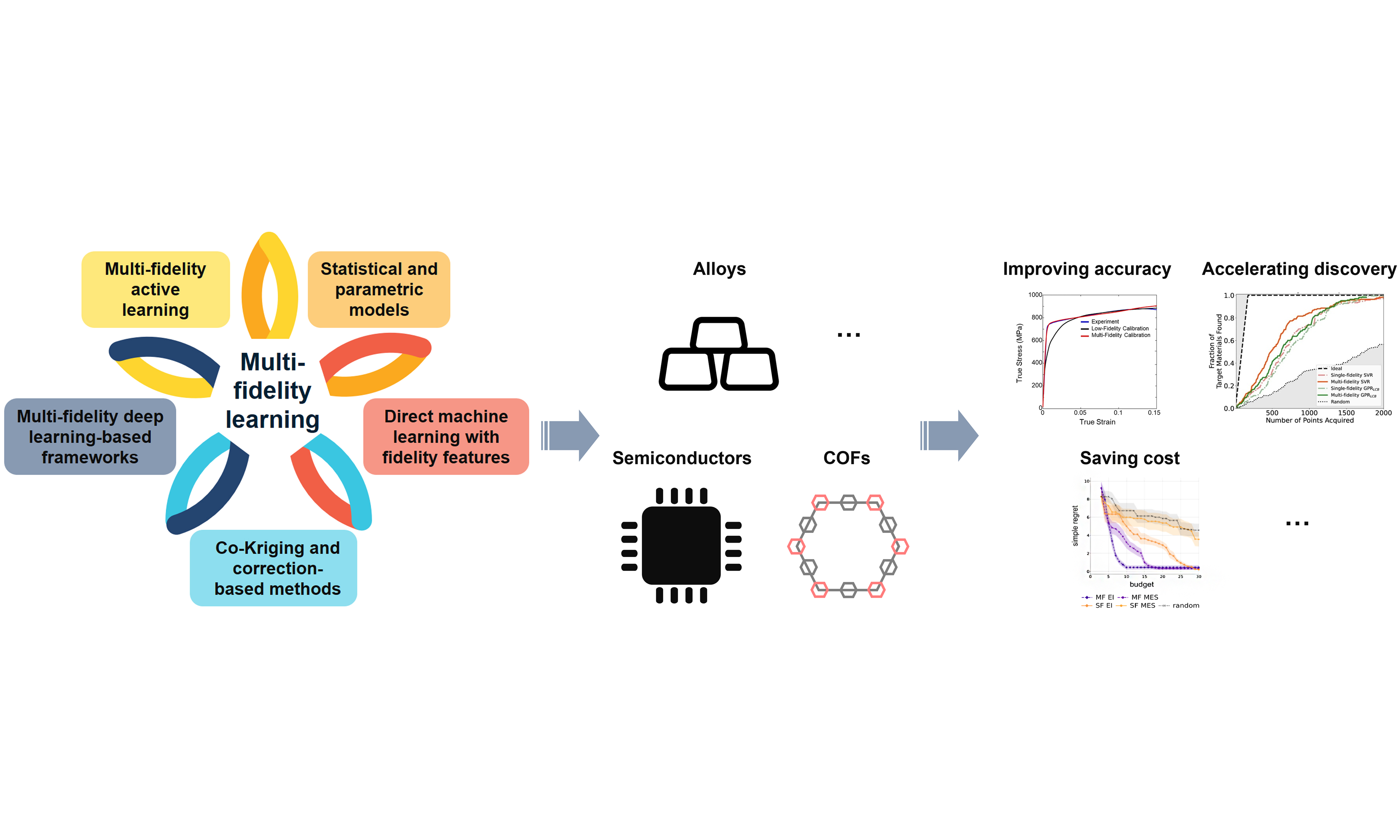
Building on these diverse applications, the purpose of this review is to provide a comprehensive overview of methodologies for MF learning in materials design. We first classify and analyze the principal strategies, illustrating each with representative case studies. We then discuss cross-cutting themes, including the handling of bias-variance trade-offs, data co-location requirements, and computational scaling. Finally, we highlight the challenges and opportunities that will shape the future of this field, from the integration with autonomous discovery systems to the development of physics-informed, generative frameworks. By consolidating methodological insights and materials applications, this review aims to guide both machine learning researchers and materials scientists toward more effective MF approaches. The principal methodological strategies are summarized in Figure 1, which also serves as a roadmap for the sections that follow.
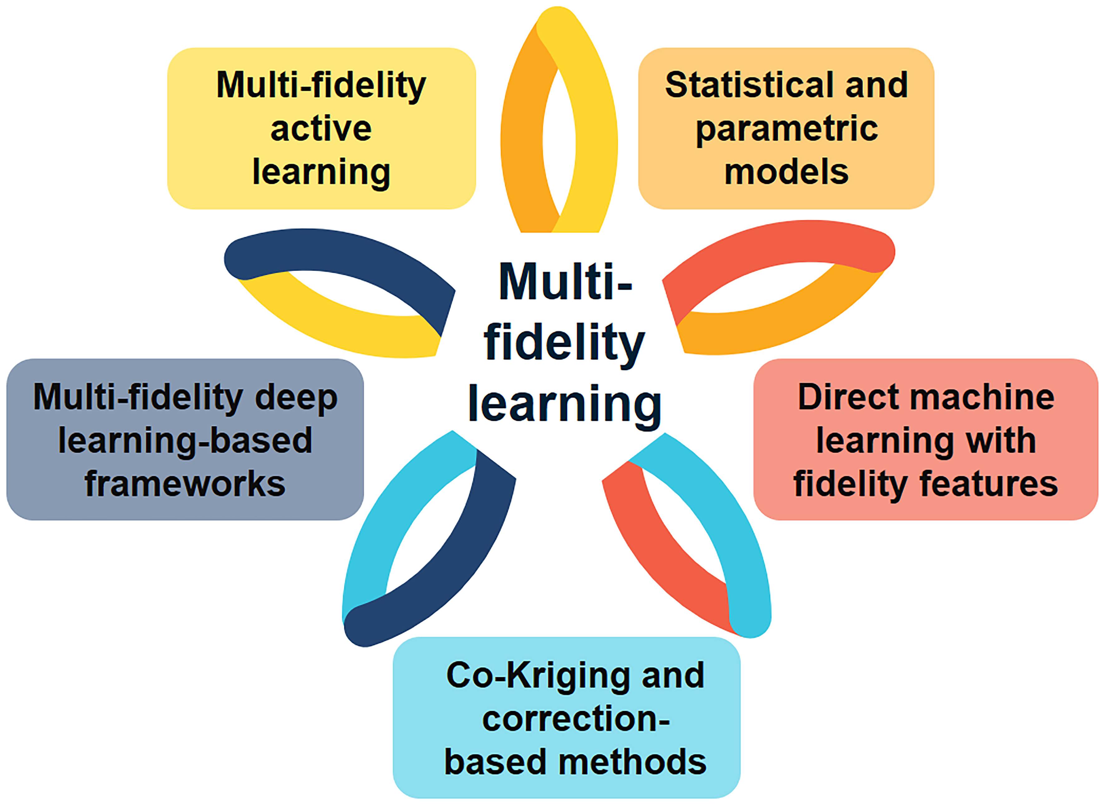
Figure 1. Taxonomy of multi-fidelity learning methodologies in materials design. Five principal strategies are highlighted: (i) Statistical and parametric models; (ii) Direct machine learning with fidelity features; (iii) Co-Kriging and correction-based methods; (iv) Multi-fidelity deep learning-based frameworks; and (v) Multi-fidelity active learning and adaptive sampling. These categories provide the structural roadmap for section “Strategies and applications for multi-fidelity learning in materials design”, where each approach is introduced, illustrated with representative case studies, and evaluated in terms of strengths, limitations, and domains of applicability.
STRATEGIES AND APPLICATIONS FOR MF LEARNING IN MATERIALS DESIGN
We classify MF learning methodologies into five broad categories[Figure 1]: statistical and parametric models, direct machine learning with fidelity features, co-kriging and correction-based methods, MF deep learning-based frameworks, and MF active learning and adaptive sampling. Each of these strategies represents a distinct way of integrating information across fidelity levels. In the subsections below, we describe their core ideas, illustrate their use with representative examples, and evaluate their strengths, weaknesses, and appropriate domains of application.
Statistical and parametric models
A classical approach to incorporating MF information is to assume an explicit functional form grounded in physical or statistical reasoning. Data at different fidelity levels are represented with distinct noise variances, which are used to fit the functional form. HF data are accurate (small noise variance) but scarce, while LF data are abundant but noisy (large noise variance). Different data are therefore weighted according to their noise levels during the fitting process, typically via maximum likelihood under fidelity-dependent noise[61,62].
A common strategy is to posit a parametric mapping y = F (x; θ) and estimate the parameters θ using maximum likelihood under fidelity-dependent noise. Concretely, one assumes
where σ2f (i) denotes the noise variance associated with the fidelity level f (i) of sample i. The corresponding log-likelihood is
where the fidelity-dependent noise variance explicitly enters the likelihood. Maximizing this fidelity-weighted Gaussian log-likelihood with respect to θ is equivalent to solving a weighted least squares problem:
This formulation makes the role of fidelity explicit: higher-variance (lower-fidelity) data points are downweighted, while HF points with smaller variance exert a stronger influence on the parameter estimates[61,62]. Thus, MF fusion is naturally achieved by adjusting the statistical weight of each fidelity level during parameter estimation.
The same variance-weighting principle also appears in GP and Kriging frameworks, where predictive means and variances from multiple fidelities are combined via inverse-variance weighting, and hyperparameters are fitted by maximum likelihood[46,63]. In these approaches, fidelity is again treated statistically, with higher-fidelity data associated with smaller predictive variance, thereby exerting a stronger influence on the posterior model. This parallel highlights a unifying view: fidelity enters the modeling process through its impact on the variance structure.
The parametric and weighted least squares treatment is attractive because it preserves interpretability and transparency. The functional form F can be chosen to encode physical insights (e.g., linear or low-order polynomial response surfaces), while MF fusion is handled systematically through the likelihood-based weighting scheme. It is also computationally efficient and, when combined with projection-enabled linear regression, can accommodate non-overlapping MF datasets in which HF and LF data are observed at different inputs[64]. When domain knowledge suggests a credible approximation form for F, parametric MF models are parsimonious, fast, and robust, providing a principled mechanism to prioritize HF data while still leveraging LF samples to capture global trends.
In practice, parametric MF models are most effective in applications where domain expertise provides guidance for a plausible functional form. For example, in hypersonic vehicle surface pressure modeling, MF linear regression improved predictive accuracy by up to 12% compared to SF regression, even with as few as 3-10 HF samples[64]. In materials science, heteroscedastic Gaussian process regression (HGPR) has been applied to porous two-phase microstructures generated by finite element simulations. In this setting, input-dependent noise captures inherently noisy regimes, linking geometric descriptors (ellipse axes, porosity, spacing) to effective stress in representative volume element (RVE) (60%-40% split for training and validation sets)[65]. This study illustrates that heteroscedasticity in materials datasets, traditionally regarded as a nuisance, can instead be leveraged as an informative signal to guide design and optimization.
These advantages, however, come with trade-offs. Parametric MF models often suffer from limited representational capacity: linear or polynomial structures may be inadequate for highly nonlinear, high-dimensional behaviors. They can also degrade when LF data introduce systematic bias or when fidelity relationships deviate significantly from simple mappings. Furthermore, mis-specified fidelity-dependent variances can undermine the intended emphasis on HF data. Such issues can be mitigated by re-estimating variance terms via maximum likelihood or by extending the framework to include fidelity-specific offsets and scaling factors[46].
From a practical standpoint, for parametric MF models, a key design choice is the selection of the functional form. A practical strategy is to start from the simplest model justified by physical insight and progressively increase complexity as needed. Candidate models can be evaluated using cross-validation, and the model that exhibits the best generalization performance is selected.
Direct machine learning with fidelity features
A second strategy for MF learning is to directly encode fidelity information as an input feature to a unified model. Rather than building separate models at each fidelity or linking them hierarchically, all data are pooled and a single model is trained with an additional “fidelity feature”. For each sample (x, y) with fidelity f ∈ {1 (highest), …, K (lowest)}, a K-dimensional one-hot vector e f is concatenated with the material descriptors xi to form the augmented input xi = [xi ǀǀ e f (i)]. At inference, setting e f = [1, 0, …, 0] yields predictions at the highest fidelity, while other encodings correspond to lower fidelities [Figure 2A]. This approach is flexible because it does not require a one-to-one correspondence of data across fidelities or a fixed model hierarchy[39,40].
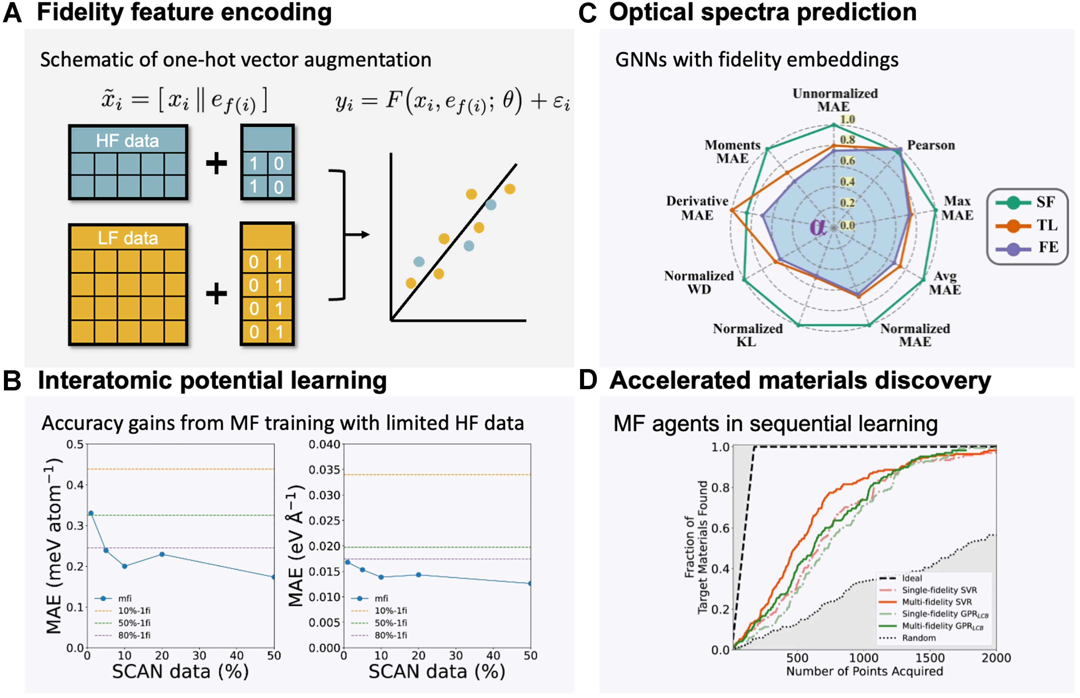
Figure 2. Examples of direct MF learning with fidelity features. (A) Schematic of the one-hot encoding fidelity approach: each sample is augmented with a fidelity indicator vector e f, allowing a single unified model to learn across low- and high-fidelity data; (B) Interatomic potential for water: test MAEs of a mfi trained with varying fractions of HF (SCAN) data (left: energy; right: force). Dashed lines indicate the MAEs of 1fi baselines using the same fractions of HF data, highlighting the efficiency of MF learning[39]; (C) Frequency-dependent optical spectra (reduced absorption coefficient α): radar charts show normalized median errors on the HF test set for three GNNs-SF, TL, and FE, demonstrating the performance gains from fidelity-aware embeddings[66]; (D) Simulated inorganic materials discovery under sequential learning: the x-axis shows the experimental acquisition budget, and the y-axis shows the fraction of ideal materials (with visible-spectrum band gaps) discovered. MF agents with fidelity indicators accelerate discovery relative to SF agents[47]. MF: Multi-fidelity; HF: high fidelity; LF: low fidelity; MAE: mean absolute error; mfi: multi-fidelity model; 1fi: single-fidelity model; SCAN: strongly constrained and appropriately normed (density functional); GNNs: graph neural networks; SF: single fidelity; TL: transfer learning; FE: fidelity embedding.
Formally, each observation can be written as
where xi denotes the material descriptors, e f (i) is the one-hot encoding of the fidelity level, and εi represents observation noise. Unlike the parametric formulations discussed in section “Statistical and parametric models”, the functional form F is not prescribed a priori. Instead, F is estimated directly from data using machine learning models such as neural networks, support vector machines, or GPs. The fidelity encoding, therefore, guides the model to integrate information across fidelities within a unified representation, rather than weighting data points through fidelity-dependent noise variances.
Direct MF learning with fidelity features has been successfully applied in several areas of materials modeling. Ko and Ong integrated fidelity information into the “global state” of a graph neural network (GNN; M3GNet) to build a MF interatomic potential. Training on combined datasets of LF and HF simulations (e.g., silicon and water), the MF M3GNet achieved the accuracy of a HF-only model using only ~10% of the HF data, representing an order-of-magnitude saving in computational cost for generating HF data [Figure 2B][39]. Kim et al. developed SevenNet-MF, an equivariant GNN trained on mixed generalized gradient approximation (GGA, LF) and meta-generalized gradient approximation (meta-GGA, HF) calculations using one-hot fidelity features. With just 10% HF data relative to the LF set, SevenNet-MF achieved < 10% error in Li-ion conductivity and R2 ≈ 0.98 for mixing energies on validation sets (90%-10% split for training and validation sets), outperforming fine-tuning and ∆-learning baselines[40]. Together, these studies demonstrate that fidelity features enable models to effectively expand HF datasets by leveraging LF trends.
The approach has also been extended beyond interatomic potentials. Ibrahim and Ataca developed a GNN for predicting frequency-dependent optical spectra by embedding fidelity information as a learnable vector. Joint training on LF and HF spectra (34,327 LF data and 14,560 HF data) significantly reduced errors on test sets (80%-5%-15% split for training-validation-test sets) in dielectric response predictions compared to HF-only training, and even outperformed transfer learning baselines[Figure 2C][66]. Similarly, in the inverse design of halide perovskites, MF surrogates with fidelity indicators guided genetic algorithms to yield experimentally stable compositions by combining generalized gradient approximation Perdew-Burke-Ernzerhof (GGA-PBE, LF, 570 data), Heyd-Scuseria-Ernzerhof hybrid functional (HSE06, HF, 347 data), and experimental measurements (alternative HF, 97 data)[56]. In high-throughput screening, multi-output GPs incorporated fidelity information by concatenating fidelity tags with material descriptors, enabling the fusion of experimental and computational measurements within a single workflow and improving both efficiency and uncertainty quantification[54]. Mora et al. encoded data sources as one-hot vectors and fed them into a Bayesian neural network that maps fidelity indicators onto a low-dimensional continuous fidelity manifold, through which uncertainty is propagated to the output layer. This formulation imposes no restriction on the number of fidelities and avoids a predefined hierarchy. The network outputs both predictive means and variances, enabling quantification of prediction uncertainty as well as fidelity-related uncertainty. Applied to MF damage simulations of porous metallic components and to binding energy prediction in hybrid organic-inorganic perovskites, the learned manifold disentangles heterogeneous data sources and yields well-calibrated uncertainty estimates[67]. Beyond deterministic surrogates, Zanjani Foumani et al. introduced a cost-aware Bayesian optimization framework with a MF emulator that one-hot encodes fidelity as a categorical variable, learns across fidelities, and automatically detects when LF sources are too biased to be useful[68]. Palizhati et al. further showed that MF agents encoding fidelity features (DFT as LF, experiments as HF) accelerated early discovery by 20%-60% compared to SF baselines [Figure 2D][47].
Overall, direct MF machine learning provides a powerful and flexible strategy for exploiting heterogeneous datasets under limited HF budgets. These approaches have already enabled the cost-effective development of interatomic potentials approaching coupled-cluster accuracy, predictors of complex optical properties, and efficient high-throughput surrogates. They can reduce HF data requirements by up to an order of magnitude while matching or even surpassing the accuracy of HF-only models[39,40]. Compared to correction-based approaches introduced in section “Co-Kriging and correction-based methods”, direct methods do not require overlapping data across fidelities; instead, they integrate complementary information within a unified representation[39,66].
Despite these strengths, several limitations remain. Encoding fidelity as a one-hot tag does not explicitly capture cross-fidelity correlations (LF→HF mapping), which reduces interpretability relative to autoregressive or correction-based models. The approach also does not inherently account for heteroscedasticity or calibration: noisy LF data can dilute the HF signal and compromise uncertainty quantification. In addition, severe class imbalance, where only a small number of HF samples are available, may lead to overfitting to LF trends or spurious correlations between fidelity and input features. Thus, while direct MF learning with fidelity features is highly flexible and data-efficient, it is most effective when LF data are reasonably correlated with HF targets and when a sufficient number of HF points are available to anchor the learning process.
From a practical standpoint, performance is also sensitive to model-specific hyperparameter choices. Hyperparameter tuning in direct MF learning depends on the underlying machine learning model. For neural networks, the primary hyperparameters include network architecture, learning rate, batch size, and regularization strength. For GPs, the dominant choices are the kernel (covariance function), its associated hyperparameters, and the noise level.
Co-kriging and correction-based methods
Correction-based methods, most prominently co-kriging, represent one of the most established strategies in MF learning[48]. They extend GP regression by modeling correlations between LF and HF data, thereby leveraging the broad coverage of inexpensive LF data to complement the accuracy of HF data. The basic idea, illustrated in Figure 3A, is to learn a statistical correction that maps LF outputs to HF outputs, effectively “lifting” cheap predictions into the accuracy regime of expensive ones. Formally, one seeks a correction operator C such that
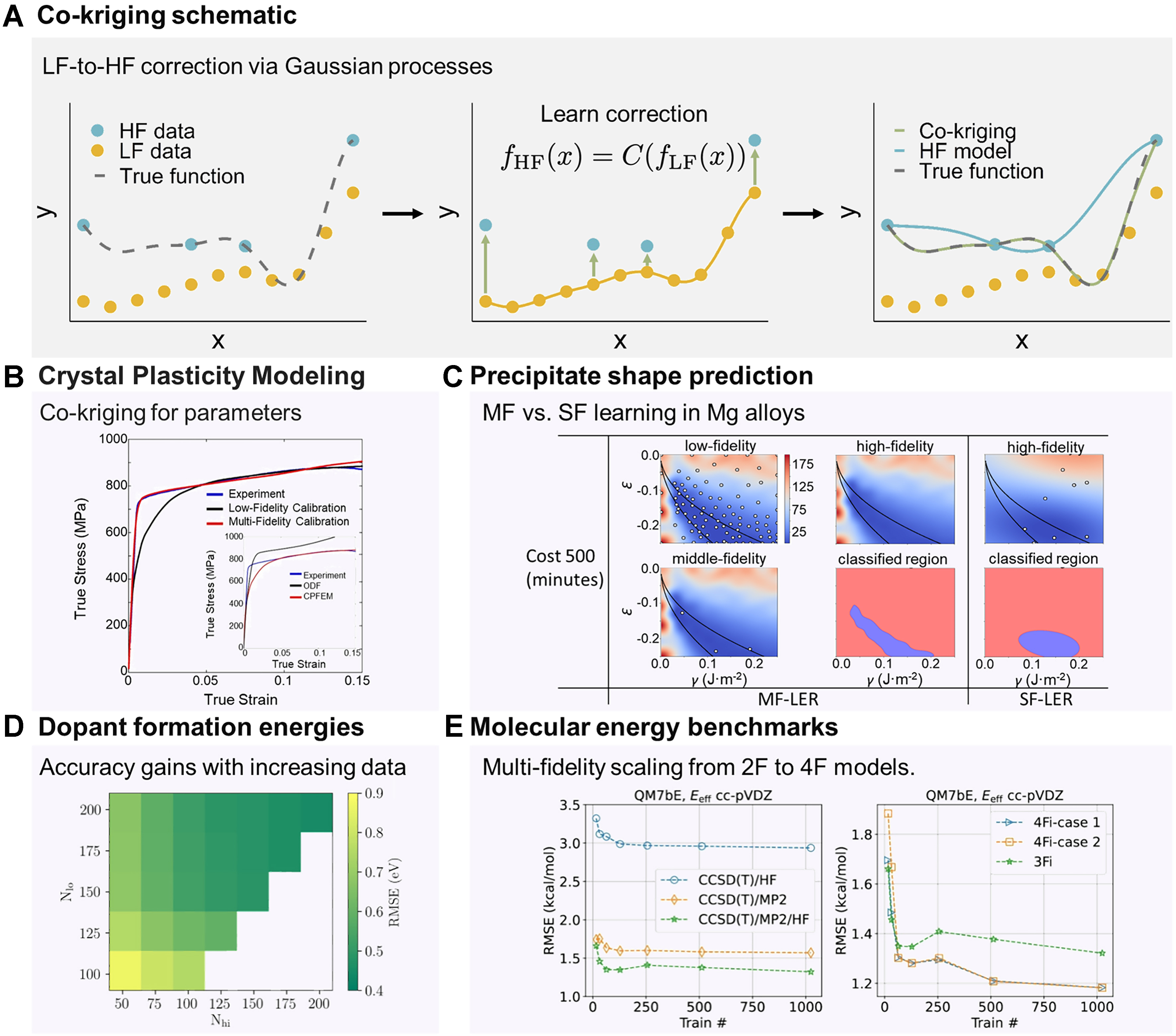
Figure 3. Examples of correction-based MF learning using co-kriging. (A) Schematic illustration of the co-kriging approach, where a GP model learns a correction that maps LF to HF responses (adapted from[71]); (B) Crystal plasticity modeling of Ti-7Al alloy: the resulting stress-strain responses indicate that the MF calculations perfectly reproduce the experimental results. The inset shows HF (CPFEM) and LF (ODF) data[77]; (C) Precipitate shape simulation in Mg alloys: heatmaps show predicted discrepancies between simulated and experimental precipitate aspect ratios. White points mark observed samples, and black lines indicate the actual LER. Binary images are predicted LERs from co-kriging (MF) and HF-only (SF) models, demonstrating that additional LF data improve efficiency[28]. The ε denotes the crystal mismatch between the precipitate and matrix phases, while γ is the interface energy; (D) Dopant formation energies in hafnia calculated using DFT: the prediction accuracy of co-kriging models improves as the number of HF (Nhi) and LF (Nlo) training points increases[34]; (E) Atomization energy benchmarks: the RMSE decreases as more fidelities are combined. Two-fidelity models use CCSD(T)/HF or CCSD(T)/MP2, while 3Fi and 4Fi models show progressively better accuracy[78]. Overall, these case studies highlight the versatility of correction-based surrogates in bridging simulations and experiments across diverse materials applications. MF: Multi-fidelity; HF: high fidelity; LF: low fidelity; SF: single fidelity; GP: Gaussian process; DFT: density functional theory; CPFEM: crystal plasticity finite element method; ODF: orientation distribution function; LER: lower-error region; RMSE: root-mean-square error; CCSD(T): coupled cluster with single, double, and perturbative triple excitations; MP2: second-order Møller-Plesset perturbation theory; 3Fi: three-fidelity; 4Fi: four-fidelity.
where C is learned from data. In co-kriging, this mapping is embedded within a GP framework so that LF and HF functions are modeled as correlated random processes, and the learned correction enables the surrogate to follow HF trends while exploiting LF coverage. The GP framework naturally provides predictive uncertainty across the input space[41,48,69-71]. In GP regression, the posterior prediction at a new input x* is Gaussian with a closed-form mean and variance, which naturally provides calibrated predictive uncertainty. Here, uncertainty reflects both data noise (aleatoric uncertainty) and limited knowledge of the underlying function (epistemic uncertainty). In materials informatics, such uncertainty-aware predictions are essential for risk-sensitive decision making and adaptive sampling, where uncertainty estimates guide the selection of new simulations or experiments. GP-based co-kriging, therefore, enables principled quantification and propagation of uncertainty across fidelity levels.
A particularly common instantiation of this correction framework is the first-order autoregressive (AR1) formulation introduced by Kennedy-O’Hagan and later popularized by Forrester[71]. In this approach, the HF function is expressed as[71]
where ρ is a scaling factor and δ (x) is an independent GP that captures the systematic LF→HF discrepancy. This formulation can be viewed as a specific parametric choice for the correction operator C (·), with LF predictions rescaled and then adjusted by an additive discrepancy term. The resulting joint GP induces a block covariance structure linking LF and HF observations, thereby enabling interpolation of HF data while rigorously quantifying predictive uncertainty. Despite its popularity, the AR1 co-kriging formulation relies on several implicit assumptions. First, the mapping between LF and HF responses is assumed to be approximately linear, such that a single scaling factor captures the dominant cross-fidelity relationship. When the LF→HF relationship is strongly nonlinear or state-dependent, this linear autoregressive assumption may break down, motivating the use of more flexible nonlinear correction operators. Second, both the LF process fLF (x) and the discrepancy term δ (x) are typically modeled as stationary GPs, meaning that their mean functions are constant and their covariance structures depend only on the separation between inputs. This co-stationarity assumption can be restrictive in systems where cross-fidelity correlations vary significantly across the input space[41,48,70,72-75]. When these linearity or stationarity assumptions are violated, alternative MF strategies may be more appropriate. Examples include nonlinear correction-based formulations, composite or deep GP models, and direct machine learning approaches with fidelity features that do not impose explicit parametric structure on LF-HF mappings. In practice, diagnosing the degree of linearity and stationarity in cross-fidelity relationships provides useful guidance for choosing among classical co-kriging, nonlinear GP variants, and deep learning-based frameworks.
There are also alternative forms of the general correction operator C (·). Recursive co-kriging extends the autoregressive framework to more than two fidelity levels by chaining GPs across coarse, intermediate, and fine datasets[48,70,72]. Composite and deep GP models enrich the operator C (·) to capture nonlinear mappings between fidelities that cannot be represented by a simple affine relation[41,73-75]. Other formulations, such as those based on radial basis functions (RBFs) or multi-output GP surrogates, have likewise been introduced, further broadening the family of correction-based strategies[76].
Co-kriging has already enabled significant advances in materials design[32,51,77-81]. In crystal plasticity, a co-kriging model combining 100 LF orientation distribution function (ODF) data with 10 HF crystal plasticity finite element method (CPFEM) simulations was used to calibrate slip and twinning parameters of Ti-7Al against tensile data, markedly improving stress-strain predictions relative to the ODF-calibrated model [Figure 3B][77]. In precipitation modeling of Mg alloys, co-kriging identified low-error regions more efficiently than HF-only surrogates [Figure 3C][28]. In electronic structure applications, it has been used to correct bandgaps computed using semi-local DFT with the Perdew-Burke-Ernzerhof (PBE) functional to the accuracy of the Heyd-Scuseria-Ernzerhof (HSE) hybrid functional, enabling HF-quality predictions for thousands of materials at a fraction of the computational cost [Figure 3D][34,42,52]. In molecular benchmarks, autoregressive GPs trained across multiple fidelities, including HF DFT, second-order Møller-Plesset perturbation theory (MP2), and coupled-cluster with singles, doubles, and perturbative triples [CCSD(T)], showed steadily decreasing errors as each fidelity level was incorporated [Figure 3E][78]. For molecular crystal prediction, co-kriging enabled the re-ranking of candidate polymorphs with hybrid DFT accuracy using only a small subset of direct calculations[33]. In alloy design, LF molecular dynamics simulations with a machine-learned potential have been combined with select HF DFT data to efficiently map composition-property relationships[82]. Battery applications have likewise benefited, where LF data from related cells informed the extrapolation of long-cycle HF degradation profiles[37]. Finally, in process engineering, analytical melt-pool models have been corrected with finite-element simulations to predict melt-pool dimensions in additive manufacturing, while in fracture mechanics, small sets of HF experimental data (6 points) have been amplified by co-kriging with inexpensive theoretical predictions (22 points)[83,84]. Together, these examples highlight the broad applicability of correction-based methods across length scales, materials classes, and property types.
Beyond specific applications, co-kriging offers several general advantages. By jointly modeling LF and HF data, it can deliver HF-level accuracy at a fraction of the computational cost, particularly when abundant LF data are available to constrain global trends. Uncertainty quantification is inherent to the GP framework and is especially valuable for downstream tasks such as active learning and Bayesian optimization. By contrast, most deep learning-based MF approaches do not provide calibrated uncertainty estimates unless explicitly augmented with probabilistic outputs, such as Bayesian neural networks or ensemble methods. Moreover, co-kriging is versatile: whenever cross-fidelity correlations exist, it can fuse heterogeneous data sources, including multiple levels of simulation, simplified analytical models, and experimental measurements. Compared with multivariate probability distribution-based MF models, co-kriging explicitly learns functional input-output relationships across fidelities, which is critical for capturing complex structure-property mappings.
Nevertheless, several practical limitations remain. Reliable calibration of the LF→HF mapping often requires overlapping (nested) data, i.e., the same inputs observed at multiple fidelity levels. When this condition cannot be satisfied, more flexible alternatives, such as direct machine learning with fidelity features or probabilistic deep learning models, may be better suited for non-nested or heterogeneous datasets. Beyond data requirements, computational scalability poses a further challenge. The training cost scales cubically with the number of samples, and the joint covariance structure grows with the number of fidelity levels, making large-scale applications computationally expensive. Interpretability can also be limited, as the discrepancy term δ (x) is a statistical adjustment that lacks direct physical meaning. Finally, simple linear autoregressive assumptions may fail when LF→HF relationships are nonlinear or strongly state-dependent, thereby motivating the development of deep or composite GP corrections. These trade-offs are important to consider when deciding between correction-based and alternative MF strategies.
From a practical perspective, the successful application of co-kriging also depends on careful hyperparameter selection and calibration. The dominant hyperparameters of co-kriging largely mirror those of GPs, including the choice of kernel (covariance function), its associated hyperparameters, and the noise level. In addition, for linear autoregressive formulations, the scaling factor ρ plays a critical role. The simplest choice is a constant ρ, which can be generalized to an input-dependent ρ (x) (e.g., linear or polynomial in x) to capture more complex corrections. Common kernel choices include exponential, radial basis function (RBF), Matérn family, and periodic kernels. If the data exhibit repeating patterns, periodic kernels are appropriate; if a smooth response is expected, exponential or RBF kernels are often preferred; conversely, for rougher behavior, Matérn 3/2 or 5/2 kernels provide reasonable starting points. Kernel hyperparameters are typically tuned via grid search or gradient-based optimization combined with cross-validation. When data are noisy or heteroscedastic across fidelity levels, separate noise parameters should be retained and jointly optimized.
MF deep learning-based frameworks
Recent advances in MF modeling have increasingly turned to deep learning architectures as flexible tools for linking LF and HF datasets in materials science, as schematically shown in Figure 4A. Unlike co-kriging or other correction-based models, neural networks can capture highly nonlinear and non-smooth relationships, making them particularly attractive for property landscapes where traditional surrogates struggle[49,85,86].
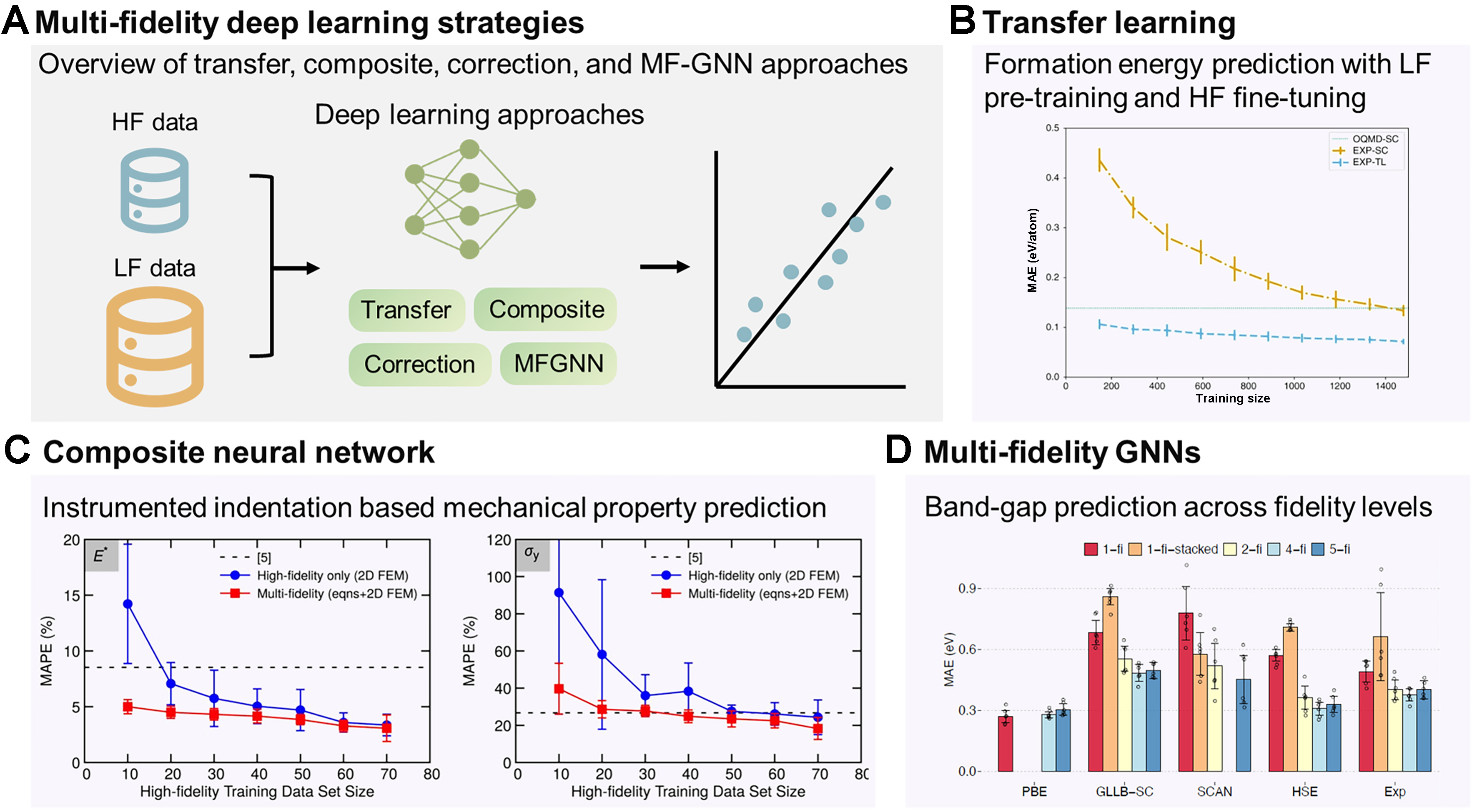
Figure 4. Deep learning-based MF frameworks for materials science. (A) Schematic overview of representative strategies: transfer learning, composite neural networks, correction learning, and MFGNN; (B) Transfer learning for formation energy prediction: performance comparison of SF models trained on the Open OQMD (LF, 341k entries) and EXP-TL. Incorporating LF knowledge reduces MAE across training sizes; results are obtained by 10-fold cross-validation, and error bars indicate the standard deviation (confidence interval) across folds[35]; (C) Composite neural network for extracting mechanical properties from indentation: MAPE as a function of training dataset size for the HF-only model and MF model, in comparison with the LF baseline (noted as [5])[30]. Reproduced from[30], © (2020) National Academy of Sciences. Distributed under the Creative Commons Attribution-NonCommercial-NoDerivatives 4.0 International (CC BY-NC-ND 4.0) license; image reused without modification; (D) MF graph neural network for band-gap prediction: comparison of MAE distributions across 1-fi, correction (1-fi-stacked), 2-fi, and MF (4-fi, 5-fi) models. LF data comprise PBE band gaps, while HF datasets include GLLB-SC, SCAN, HSE, and experimental values. Increasing fidelity integration systematically lowers prediction error[29]. Reproduced from[29] under the Creative Commons Attribution-ShareAlike (CC BY-SA 4.0) license. Together, these examples highlight the versatility of deep learning architectures in capturing nonlinear correlations and leveraging heterogeneous datasets for improved accuracy in MF learning. MF: Multi-fidelity; HF: high fidelity; LF: low fidelity; SF: single fidelity; GNN: graph neural network; MFGNN: multi-fidelity graph neural network; OQMD: Open Quantum Materials Database; TL: transfer learning; EXP-TL: experimental data (HF) with a transfer-learned model; MAE: mean absolute error; MAPE: mean absolute percentage error; PBE: Perdew-Burke-Ernzerhof (functional); GLLB-SC: Gritsenko-van Leeuwen-van Lenthe-Baerends solid-correlation (functional); SCAN: strongly constrained and appropriately normed (functional); HSE: Heyd-Scuseria-Ernzerhof (hybrid functional); 1-fi: single-fidelity; 2-fi: two-fidelity; 4-fi: four-fidelity; 5-fi: five-fidelity.
One important strategy is transfer learning between simulation tiers or between simulations and experiments. A common paradigm involves pretraining a deep neural network (DNN) on abundant LF data, followed by fine-tuning selected layers using limited HF data, sometimes with physics-informed constraints[87-89]. For example, Chakraborty proposed a MF physics-informed deep neural network (MF-PIDNN) that encodes approximate physical laws at the LF level and is subsequently updated using scarce HF data, demonstrating reliable predictions in reliability analysis where experiments are limited but governing physics is known[88]. In materials applications, this approach has been used for mechanical property inference from small punch tests, polymer property prediction using heterogeneous data sources, and formation energy prediction, where DFT pretraining accelerates learning on scarce experimental labels [Figure 4B][35,43,57]. Similar paradigms have been applied to fatigue life prediction with small datasets[90] and even cross-domain transfer from inorganic datasets to metal-organic frameworks, where pretraining on one materials domain accelerates discovery in another[55]. The latter study provides concrete validation of the generalization capability of MF transfer learning, demonstrating that latent representations learned from one class of materials can be reused in chemically distinct domains. Such transfer substantially reduces HF data requirements when exploring new materials families and highlights the robustness of MF representations beyond narrowly defined training distributions.
While transfer learning leverages sequential training, an alternative approach is to integrate multiple fidelities simultaneously within a composite neural network[49]. Islam et al.[91] demonstrated this concept for molecular dynamics, where coarse time-step data serve as LF inputs and fine time-step results provide HF corrections, yielding accurate pressure predictions with reduced computational time cost. To assess not only accuracy but also reliability, the authors evaluated model stability under repeated training. For each training-set size, the networks were retrained multiple times using different random selections of HF data while keeping the LF dataset fixed (10,000 samples for E* or 100,000 samples for σ y). The error bars in Figure 4C report the standard deviation of the resulting mean absolute percentage error (MAPE) across these repeated trainings, thereby quantifying variability in generalization performance. The substantially narrower error bars observed for MF models indicate more stable predictions and higher reliability under changes in the HF training subset. This example illustrates that, beyond improving mean accuracy, MF learning can significantly enhance robustness and reduce sensitivity to data selection[30]. Similar frameworks have been applied to predict the residual strength of graded composites and to recover stress-strain fields from digital image correlation in welds, all by coupling simulated and experimental data within a unified deep network[36,92]. These studies show how composite neural networks exploit correlations between fidelities to deliver robust surrogates that outperform HF-only training at much lower cost.
A related approach is correction learning, where a network is trained directly on the discrepancy between LF and HF predictions. In band-gap benchmark studies, this strategy achieved lower errors than both transfer learning and composite neural networks, as the model concentrates its capacity on systematic LF bias[93]. However, correction learning requires nested LF/HF pairs for training and typically demands an LF evaluation for every new query, which can limit its applicability when LF evaluations are computationally expensive.
Building on these approaches, the most ambitious efforts extend deep learning into MF GNNs. Chen et al. incorporated fidelity tags into the Materials Graph Network (MEGNet) to learn across band-gap datasets ranging from the PBE (LF) functional to the HSE hybrid functional and experimental measurements (HF)[29]. By embedding fidelity as a global state, their model integrates heterogeneous datasets and captures correlations across fidelity levels. As shown in Figure 4D, MF GNNs consistently outperform SF and stacking models. Performance is evaluated on randomly segmented test sets (80%-10%-10% split for training-validation-test sets, repeating 6 runs), where the error bars show one standard deviation across runs (confidence intervals) and the dots denote individual model errors. Beyond the common two-level low- and HF setting, the effect of introducing multiple intermediate fidelity levels has been systematically examined. As additional fidelities are incorporated, prediction errors generally decrease and uncertainty bands narrow, reflecting improved regularization of the shared latent representation. However, adding a fidelity level with very limited data or weak correlation can degrade performance, as observed when a small SCAN dataset was included. This finding illustrates that increasing the number of fidelities is beneficial only when the added levels contribute sufficient data volume and maintain meaningful correlation with existing fidelities. These graph-based frameworks are particularly suited to materials discovery, as they naturally represent atomic topology while allowing fidelity-specific corrections.
Deep learning-based MF frameworks therefore provide remarkable flexibility in handling heterogeneous and non-nested data, while capturing strongly nonlinear trends that challenge traditional surrogates. At the same time, they are computationally intensive, sensitive to hyperparameter choices, and often lack interpretability, which motivates the continued integration of physics-based constraints to mitigate small-data challenges[94]. Overall, these methods are emerging as powerful tools in materials science, particularly in scenarios involving strong nonlinearity, heterogeneous datasets, and the need for rapid discovery. By coupling the adaptability of deep learning with domain knowledge, MF neural frameworks are poised to become indispensable for next-generation materials design.
From a practical standpoint, the effectiveness of deep learning-based MF frameworks depends strongly on careful hyperparameter selection and training strategies. In practice, their effective deployment requires strategy-specific hyperparameter tuning. For transfer learning, a common approach is to stabilize the shared representation using abundant LF data, followed by limited fine-tuning with HF labels. When HF data are scarce, freezing early layers is often beneficial. For composite neural networks, loss weighting should prioritize HF accuracy while still retaining LF trend learning; a practical strategy is to begin with HF-weighted objectives and gradually relax toward a balanced multi-task loss. Throughout training, both accuracy and probabilistic metrics (e.g., negative log-likelihood and prediction interval coverage) should be monitored to ensure that uncertainty calibration does not degrade as LF information is incorporated. For correction learning, residual blocks should be kept lightweight, with sufficient capacity to capture systematic LF→HF discrepancies without overfitting. For MF GNNs, fidelity embeddings should remain compact and be jointly tuned with the shared trunk so that they modulate predictions without overwhelming structural features. In general, modest and budgeted hyperparameter searches focused on learning rate, weight decay, and loss weights (guided by HF validation and uncertainty calibration) tend to yield larger gains than aggressive architectural changes, particularly when HF data are limited.
MF active learning and adaptive sampling
Active learning and adaptive sampling extend MF modeling into a dynamic, decision-making context. Rather than passively integrating heterogeneous datasets, these approaches sequentially decide not only which candidate material to evaluate next, but also at which fidelity level [Figure 5A]. The central objective is to maximize the expected information gain per unit cost, thereby accelerating discovery while respecting finite computational and experimental budgets.
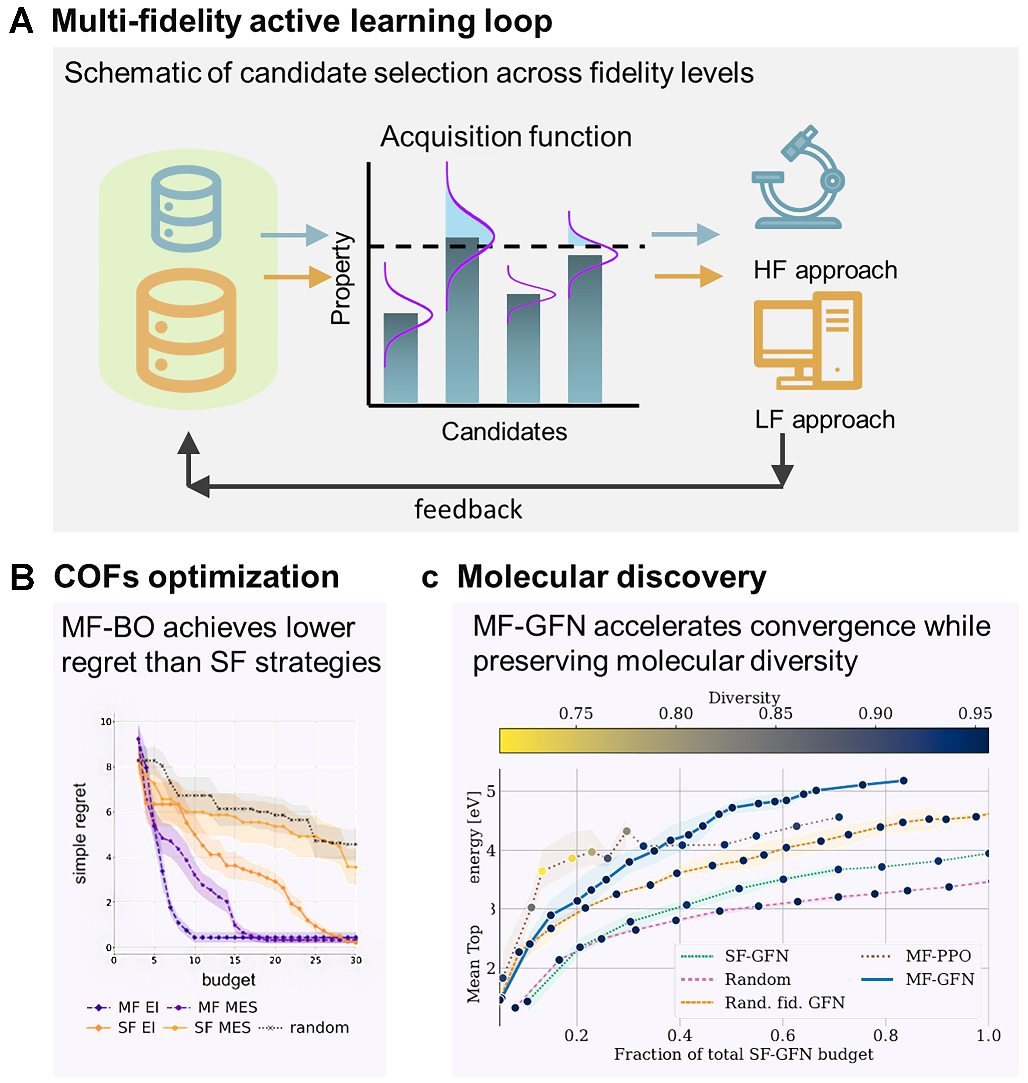
Figure 5. MF active learning and adaptive sampling in materials science. (A) Active-learning loop: schematic of candidate selection and fidelity allocation, where promising candidates are evaluated with costly HF methods and less valuable candidates with inexpensive LF approximations; (B) COF optimization: MF active learning achieves lower simple regret for xenon-krypton selectivity compared to SF and random baselines[60]; (C) Molecular discovery: MF-GFN accelerate convergence toward diverse molecules with desirable electron affinity compared with SF and random-fidelity approaches[96]. Together, these examples illustrate how MF active learning dynamically balances exploration, exploitation, and cost to accelerate discovery across molecular and porous materials. MF: Multi-fidelity; HF: high fidelity; LF: low fidelity; SF: single-fidelity; MF-BO: multi-fidelity Bayesian optimization; COF: covalent organic framework; GFN: generative flow network; MF-GFN: multi-fidelity generative flow network; SF-GFN: single-fidelity generative flow network; PPO: proximal policy optimization; MF-PPO: multi-fidelity proximal policy optimization; MES: max-value entropy search; MF-MES: multi-fidelity max-value entropy search; EI: expected improvement; SFEI: single-fidelity expected improvement.
A central paradigm is multi-fidelity Bayesian optimization (MF-BO), in which GP surrogates or deep-kernel variants model correlations between fidelity levels [Table 1][50]. Acquisition functions are adapted to weigh both evaluation cost and expected improvement (EI), enabling the algorithm to alternate between inexpensive LF approximations and costly HF evaluations[50]. For example, MUlti-task Max-value Bayesian Optimization (MUMBO) employs a cost-aware acquisition function that selects the candidate-fidelity pair expected to deliver the largest reduction in uncertainty about the global optimum per unit cost, scaling effectively to multi-task and MF settings[50]. Let (x, z) denote a material candidate x evaluated at fidelity level z. The next query (xn+1, zn+1) is chosen according to[50]
Pseudo code of MF-BO
| 1: | Given design space |
| 2: | Start MF-BO loop |
| 3: | n ← 0, D ← D0, spent_cost ← 0 |
| 4: | while spent_cost < B and stopping criterion not met do |
| 5: | Fit multi-fidelity surrogate sn ← |
| 6: | for many candidate pairs (x, z) sampled from |
| 7: | Use sn to obtain the predictive distribution of the target property at (x, z) |
| 8: | Compute acquisition value αn (x, z) based on this predictive distribution |
| 9: | Compute cost-aware score: score(x, z) ← αn (x, z) / c (x, z) |
| 10: | end for |
| 11: | Select next evaluation pair (xnext, znext) ← arg max(x, z) score(x, z) |
| 12: | Query simulator / experiment at the chosen fidelity |
| 13: | ynext ← evaluate_material (xnext, znext) |
| 14: | Update dataset and budget |
| 15: | D ← D ∪ {(xnext, znext, ynext)} |
| 16: | spent_cost ← spent_cost + c (xnext, znext) |
| 17: | n ← n + 1 |
| 18: | end while |
where αn (x, z) is an acquisition function quantifying the EI of the target property at iteration n, and c (x, z) is a cost function associated with fidelity z[50]. This explicit balance between information gain and evaluation cost allows the algorithm to dynamically allocate resources across fidelities, alternating between LF approximations and HF evaluations[50].
Applications in materials science highlight the versatility of these strategies. In materials screening, multi-output GPs have been used to fuse experimental and computational data on-the-fly, replacing rigid stagewise funnels with progressive, budget-aware exploration and cutting optimization costs by nearly threefold in benchmark studies[54]. In covalent organic framework (COF) optimization, MF-BO achieved lower regret at a given budget compared to SF baselines, as shown in Figure 5B. To assess both average performance and reliability, MF and SF active learning strategies were evaluated using 20 independent random seeds, corresponding to different initial samples and acquisition trajectories. In Figure 5B, the shaded regions represent the standard deviation of simple regret at each budget level, capturing the spread of optimization outcomes across repeated campaigns. The visibly narrower shaded bands for MF strategies compared to their SF counterparts indicate reduced run-to-run variability and therefore higher reliability. These results highlight that MF active learning not only accelerates convergence but also yields more reproducible and dependable discovery trajectories[60].
Sequential learners extend this idea by combining regressors such as GPs, random forests, and support vector machines into active loops that adaptively decide whether to query a fast DFT simulation (LF) or a costly experiment (HF), with successful demonstrations in two-fidelity band-gap discovery agents[47]. In structural materials, MF-BO has been applied to dual-phase steel design, where LF micromechanical models (isostrain, isostress, isowork, secant, elastic-constraint) were queried far more often than costly finite element method (FEM) simulations (with RVE), especially in early iterations[53,95]. Similarly, in interatomic potential development under extreme conditions, adaptive MF sampling efficiently identified promising parameter regimes that would have been infeasible to explore exhaustively[38]. Recent innovations further embed these principles into generative frameworks. In the multi-fidelity generative flow network (MF-GFN), the acquisition function is treated as a reward signal that guides stochastic generation of candidate-fidelity tuples, enabling discovery of diverse, high-performing materials while maintaining cost efficiency and outperforming random or SF baselines [Figure 5C][96].
The strengths of MF active learning lie in its ability to allocate resources efficiently. By dynamically balancing exploration of uncertain regions with exploitation of promising candidates, these methods accelerate discovery trajectories compared to static or fixed-fidelity sampling. They are particularly well-suited for autonomous experimental laboratories and adaptive simulation campaigns, where real-time decisions about the next measurement are essential.
The main challenges arise from implementation complexity and the need for robust uncertainty quantification. Acquisition functions must be carefully calibrated to avoid over-exploitation of biased LF data and to maintain trustworthy uncertainty estimates in high-dimensional, structured search spaces. Surrogate models that combine diverse fidelities can also become computationally demanding when embedded in sequential loops. Studies have shown that while approximate LF solvers can accelerate discovery, they may also mislead active learning if correlations with HF targets are not explicitly modeled[97]. Dimensionality is another bottleneck. Recent advances such as adaptive active-subspace methods embedded within MF-BO have improved efficiency by reducing the search to informative subspaces in process-structure-property optimization[95]. Overall, MF active learning and adaptive sampling represent a critical step toward autonomous, closed-loop materials discovery, where algorithms not only predict outcomes but also decide the most efficient way to generate new data.
From a practical perspective, effective deployment of MF active learning benefits from staged hyperparameter tuning. A recommended workflow is to first stabilize the MF surrogate and cost models to ensure reliable predictions and uncertainty estimates. Next, the acquisition function should be calibrated to balance expected information gain against evaluation expense. Finally, scheduling parameters such as stopping criteria, fidelity budgets, or query ratios can be defined. In practice, a useful starting point is to pair a well-calibrated MF surrogate with a simple cost model, for example, based on computational time or dataset size.
The choice of acquisition strategy should align with the problem constraints and fidelity structure. Information-gain-per-cost criteria (e.g., entropy-based methods or MF knowledge-gradient) are robust when fidelities differ strongly in accuracy and cost, whereas EI-per-cost or Upper Confidence Bound (UCB)-per-cost strategies are effective when costs are relatively stationary across the domain. Stopping criteria can be organized into three practical tiers. Budget-based termination (e.g., fixed wall-time, total cost, or number of HF evaluations) is the default in autonomous campaigns with predefined resource limits. Progress-based criteria monitor the learning signal, such as halting when the maximum EI (or EI-per-cost) remains below a threshold for several iterations, or when posterior uncertainty in the region of interest falls below a prescribed margin. Finally, value-of-information (VoI)-based stopping rules compare the expected knowledge gain per unit cost against a minimum acceptable return and terminate when further evaluations are no longer justified. The VoI-based strategies, including cost-aware knowledge-gradient variants, are particularly suitable when cost, risk, and uncertainty must be explicitly balanced.
CROSS-CUTTING THEMES
Bias vs. variance
Compared with HF data, LF sources typically exhibit larger errors, which can be decomposed into bias and variance. Bias refers to systematic deviations introduced by differences in data-generation pipelines, such as experiments vs. simulations, simplified physical models, alternative algorithms (e.g., HSE vs. PBE), or choices of simulation hyperparameters[29,32-34,52,82,91,95,98,99]. Variance, by contrast, reflects random measurement noise and is generally lower in HF data. Examples include measurements made under the same protocol but carried out by novice vs. experienced researchers, or using worn vs. newly calibrated instruments[100].
The relative contributions of bias and variance strongly influence the choice of MF methodology, as shown in Table 2. When systematic bias dominates, correction-based methods are particularly effective because they explicitly model cross-fidelity discrepancies. Deep learning approaches or models with explicit fidelity indicators (e.g., one-hot encoding) can play a similar role by learning fidelity-specific corrections. When variance is the primary concern, statistical approaches with heteroscedastic modeling or inverse-variance weighting provide a principled treatment. In practice, especially in experimental materials data, bias and variance almost always coexist[101]. In such mixed settings, kriging-based methods (e.g., co-kriging), which simultaneously capture cross-fidelity correlations and account for heteroscedastic errors, are attractive options[48]. Active learning strategies also provide robust solutions, as they can adaptively downweight LF inputs in non-critical regions without requiring explicit assumptions about error type.
Comparison of multi-fidelity strategies across advantages, limitations, bias-variance focus, and data requirements
| Strategy | Advantages | Limitations | Bias/Variance | Data requirements |
| Statistical weighting | Simple, interpretable | Limited expressiveness | Variance | Non-nested, flexible |
| Direct ML with fidelity features | Flexible, leverages features | May underperform with sparse HF data | Bias | Works with non-nested |
| Correction-based (e.g., co-kriging) | Captures correlations, uncertainty quantification | Needs nested data, heavy compute | Both | Best with nested |
| Deep learning frameworks | Captures complex relations | Needs large datasets, less interpretable | Bias | Non-nested, but data-hungry |
| Active learning / adaptive sampling | Sample-efficient, reduces cost | Complex acquisition design | Both | Few samples; can create nested adaptively |
Overall, recognizing whether bias, variance, or both dominate a MF dataset is essential for selecting an appropriate strategy, and remains a central cross-cutting theme in the design of effective materials informatics workflows.
Data requirements: nested vs. non-nested
In addition to error characteristics, the feasibility of MF methods is strongly influenced by their data requirements, particularly the distinction between nested and non-nested designs. In a nested design, the same input x is observed at multiple fidelity levels, allowing direct comparison and correction between low- and HF outputs. By contrast, in a non-nested design, most inputs are observed at only one fidelity level, leaving little or no overlap across fidelities.
Correction-based methods such as co-kriging are especially sensitive to this distinction, as they typically assume a nested structure to learn systematic deviations between fidelities. In practice, however, materials datasets are often non-nested, arising from disparate sources such as separate DFT databases, experimental measurements, or high-throughput simulations conducted with different parameter sets. This lack of overlap makes direct discrepancy modeling challenging and can reduce the effectiveness of classical co-kriging.
To address these challenges, several extensions have been proposed that relax the nesting requirement. Specifically, recursive variants of classical co-kriging can propagate correlations across multiple fidelity levels without requiring strict nesting of input locations[48]. In the Augmented Bayesian Treed Co-Kriging (ABTCK) framework, missing cross-fidelity pairings are statistically imputed through hierarchical partitioning of the input space, creating an augmented dataset in which the joint posterior can be factorized. This approach enables fully Bayesian predictive inference under non-nested designs without enforcing explicit co-location[102]. Beyond ABTCK, the Generalized Co-Kriging (GCK) framework aggregates a calibrated LF Kriging model with a stochastic discrepancy Kriging term, such that the LF predictive distribution (mean and variance) is propagated to locations where only HF observations are available. This probabilistic coupling permits separate parameter estimation for each fidelity and enables robust fusion under both nested and non-nested conditions, improving accuracy and stability relative to classical AR1 formulations when LF-HF correlations are imperfect[103]. These methods are particularly useful in materials science, where integrating heterogeneous datasets, such as semi-local DFT with hybrid-functional calculations, or simulations with experiments, rarely yields perfectly aligned input sets.
It is important to note, however, that not all MF strategies depend on nested data. For example, statistical weighting and direct machine learning with fidelity features can operate on non-nested datasets. Deep learning frameworks provide additional flexibility, as architectures such as hierarchical neural operators or graph-based encoders can learn shared latent spaces even when input sets across fidelities do not overlap; however, such approaches typically require larger training datasets to generalize reliably. In contrast, active learning and adaptive sampling are particularly suitable for few-sample scenarios, as they strategically select HF evaluations to maximize information gain and can dynamically create nested datasets when needed. As summarized in Table 2, the degree of nesting required varies widely across methodologies, underscoring the need for approaches that can exploit both nested and non-nested data in real-world materials design.
Computational cost and scalability
The computational demands of MF algorithms vary widely, and scalability is often a decisive factor in method selection. Kriging-based approaches, including co-kriging, require inversion of an n × n covariance matrix, where n is the number of data points. As a result, training time scales as
By contrast, deep learning-based MF models can be trained using mini-batch stochastic gradient descent, for which the per-iteration computational cost scales approximately linearly with the batch size B and the number of trainable parameters P [i.e.,
In summary, while kriging-based methods provide strong uncertainty quantification and interpretability, their poor scalability necessitates caution when applied to large datasets. Neural networks and other scalable surrogates offer practical alternatives in data-rich regimes, making computational cost a central criterion when choosing among MF methodologies.
OUTLOOK: CHALLENGES AND OPPORTUNITIES
This section outlines both the challenges that constrain current progress and the opportunities that may define the future of MF learning in materials design.
Despite notable progress, several fundamental challenges remain. First, data scarcity and imbalance are persistent barriers. HF data, whether from advanced simulations or experiments, remain expensive and unevenly distributed across material classes. The absence of standardized benchmarks further complicates fair comparison among methodologies, slowing methodological innovation and adoption.
High dimensionality further exacerbates effective data scarcity in MF learning. As the number of compositional, structural, and processing descriptors grows, the design space expands rapidly, increasing the amount of data required for reliable surrogate modeling. This challenge is particularly pronounced for MF methods, where accurate learning of LF-HF correlations often relies on co-located observations in high-dimensional spaces. As a result, simply adding more LF data may yield only limited benefits. This motivates MF strategies that aim to reduce the effective dimensionality of the problem, for example, through physics-informed feature engineering, active-subspace or manifold identification, and learned latent representations.
Beyond data volume and dimensionality, incomplete or partially observed feature sets also induce an implicit degradation of data fidelity. When key compositional, microstructural, processing, or environmental descriptors are missing, physically distinct material states may collapse onto similar representations in feature space, inflating epistemic uncertainty in poorly characterized regions. In heterogeneous materials databases, records with more complete descriptor sets can therefore be regarded as higher-fidelity observations, whereas samples with missing variables represent degraded-fidelity views that should be treated explicitly rather than discarded. For example, Ching and Phoon employed a hierarchical Bayesian framework with Gibbs sampling to infer missing feature values prior to MF fusion, demonstrating improved robustness and predictive performance when only partial variables are available. This perspective highlights a fundamental connection between data completeness and fidelity and motivates future MF frameworks that jointly address missing-data inference and fidelity-aware learning[105].
Second, transferability across material classes and design domains is limited. Models trained on MF datasets for alloys or oxides, for example, may not generalize to polymers or energy-storage materials without extensive retraining.
This lack of universality reflects both intrinsic differences in physics across classes and the difficulty of encoding fidelity relationships in a transferable manner.
Third, interpretability and trust in black-box methods remain major obstacles. Deep-learning frameworks can achieve impressive accuracy in MF prediction tasks, but their opaque decision making makes it difficult to diagnose when LF biases are propagating unchecked. Without greater transparency and interpretability, the adoption of these methods in high-stakes applications, such as structural materials or energy technologies, will remain limited.
A particularly salient theme is the integration of MF methods with automated laboratories and closed-loop workflows. On the one hand, current approaches face significant barriers: to guide experiments in real time, models must not only be accurate but also computationally efficient, uncertainty-aware, and robust to noisy data streams. In addition, practical deployment requires standardized data-exchange protocols, which are still lacking. On the other hand, overcoming these challenges would make MF learning the core intelligence layer of autonomous discovery platforms. Such integration promises to reduce costs, accelerate timelines, and open pathways to discovery that are inaccessible through traditional trial-and-error workflows.
These key challenges are summarized schematically in Figure 6, which also highlights the corresponding opportunities. At the same time, these challenges create avenues for innovation. Physics-informed MF models represent a particularly promising direction, embedding domain knowledge into statistical or neural architectures to improve both accuracy and interpretability. Generative models, including diffusion models and variational autoencoders, offer new possibilities for sampling candidate materials across fidelities and for data augmentation when HF samples are scarce.
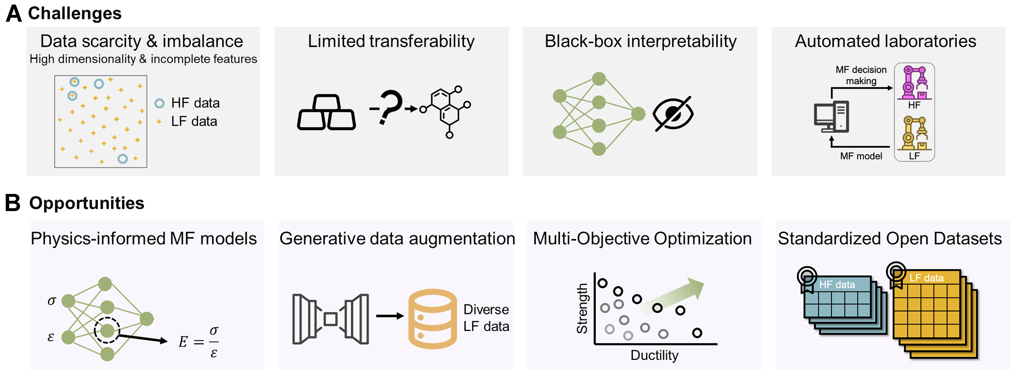
Figure 6. Conceptual summary of challenges and opportunities for MF learning in materials design. (A) Challenges: key barriers include data scarcity and imbalance between HF and LF datasets, limited transferability across material domains, the difficulty of interpreting black-box models, and integration with automated laboratories; (B) Opportunities: promising directions involve physics-informed MF models that embed domain knowledge, generative approaches for data augmentation, multi-objective optimization frameworks, standardized open datasets of HF and LF data, and coupling with autonomous discovery platforms. Together, these challenges and opportunities define a roadmap for advancing MF learning as a central tool in next-generation materials discovery.
Another important frontier is multi-objective and multi-property optimization. Real-world materials design rarely targets a single property, and extending MF frameworks to balance competing objectives, such as strength and ductility in alloys or conductivity and stability in batteries, will substantially expand their practical relevance.
Standardization of open MF datasets is also crucial. Community-wide benchmarks, analogous to those in computer vision or natural language processing, would accelerate progress by enabling direct comparison of algorithms under eproducible conditions. Such datasets could also serve as training grounds for transfer learning across material classes.
Reducing cost in MF learning typically entails fewer HF evaluations, which can increase epistemic uncertainty, particularly in regions of the input space that are sparsely sampled by HF data. MF models partially mitigate this effect by using abundant LF data to constrain the hypothesis space, but they cannot fully substitute for missing HF information. This inherent trade-off between cost and uncertainty motivates the development of cost-aware and uncertainty-aware strategies, such as MF active learning, which aim to maximize uncertainty reduction per unit cost rather than minimizing cost alone.
In summary, while MF learning in materials design faces significant challenges, it also offers a unique confluence of opportunities. Together, these challenges and opportunities define a roadmap for advancing MF learning as a central tool in next-generation materials discovery.
CONCLUSION
This review provides a structured overview of MF learning methodologies for accelerating data-driven materials modeling, design, and discovery. We summarize the major classes of MF approaches, including statistical and parametric models, direct machine learning with fidelity features, correction-based methods such as co-kriging, deep learning frameworks, and MF active learning and Bayesian optimization. Across these methods, we highlight how heterogeneous data sources can be integrated to exploit cross-fidelity correlations, improve predictive accuracy, and reduce reliance on costly HF data. Key practical considerations are also discussed, including data organization, uncertainty quantification, scalability, and integration with adaptive sampling. Looking ahead, advances in physics-informed modeling, generative methods, standardized MF datasets, and autonomous experimentation are expected to further expand the impact of MF learning. Collectively, these developments position MF approaches as a central component of efficient, reliable, and closed-loop materials discovery workflows.
DECLARATIONS
Authors’ contributions
Prepared the initial draft of the manuscript. Wang, B.; Xue, D.
Contributed to the conception and design of the review: Wang, B.; Xu, Y.; Zhou, Y.; Xue, D.
All authors participated in revising and improving the manuscript.
Availability of data and materials
Not applicable.
AI and AI-assisted tools statement
Not applicable.
Financial support and sponsorship
This work was supported by the National Key Research and Development Program of China (2021YFB3802100), the National Natural Science Foundation of China (Nos. 52573255, 92570301, 52271190, and 524B200280), the Innovation Capability Support Program of Shaanxi (2024ZG-GCZX-01(1)-06), and the Natural Science Foundation Project of Shaanxi Province (Grant No. 2022JM-205).
Conflicts of interest
Xue, D. is a Youth Editorial Board Member of Journal of Materials Informatics, but was not involved in any steps of the editorial process, notably including reviewer selection, manuscript handling, or decision making. The other authors declared that there are no conflicts of interest.
Ethical approval and consent to participate
Not applicable.
Consent for publication
Not applicable.
Copyright
© The Author(s) 2026.
REFERENCES
1. Batra, R.; Song, L.; Ramprasad, R. Emerging materials intelligence ecosystems propelled by machine learning. Nat. Rev. Mater. 2020, 6, 655-78.
2. Rao, Z.; Tung, P. Y.; Xie, R.; et al. Machine learning-enabled high-entropy alloy discovery. Science 2022, 378, 78-85.
3. Sohail, Y.; Zhang, C.; Xue, D.; et al. Machine-learning design of ductile FeNiCoAlTa alloys with high strength. Nature 2025, 643, 119-24.
4. Wang, T.; Pan, R.; Martins, M. L.; et al. Machine-learning-assisted material discovery of oxygen-rich highly porous carbon active materials for aqueous supercapacitors. Nat. Commun. 2023, 14, 4607.
5. Wu, J.; Torresi, L.; Hu, M.; et al. Inverse design workflow discovers hole-transport materials tailored for perovskite solar cells. Science. 2024, 386, 1256-64.
6. Tian, Y.; Hu, B.; Dang, P.; Pang, J.; Zhou, Y.; Xue, D. Noise-aware active learning to develop high-temperature shape memory alloys with large latent heat. Adv. Sci. 2024, 11, e2406216.
7. Xian, Y.; Dang, P.; Tian, Y.; et al. Compositional design of multicomponent alloys using reinforcement learning. Acta. Mater. 2024, 274, 120017.
8. Wei, Q.; Cao, B.; Yuan, H.; et al. Divide and conquer: machine learning accelerated design of lead-free solder alloys with high strength and high ductility. npj. Comput. Mater. 2023, 9, 201.
9. Gong, X.; Louie, S. G.; Duan, W.; Xu, Y. Generalizing deep learning electronic structure calculation to the plane-wave basis. Nat. Comput. Sci. 2024, 4, 752-60.
10. Dang, L.; He, X.; Tang, D.; Xin, H.; Wu, B. A fatigue life prediction framework of laser-directed energy deposition Ti-6Al-4V based on physics-informed neural network. IJSI 2025, 16, 327-54.
11. Rasul, A.; Karuppanan, S.; Perumal, V.; Ovinis, M.; Iqbal, M. An artificial neural network model for determining stress concentration factors for fatigue design of tubular T-joint under compressive loads. IJSI 2024, 15, 633-52.
12. Yuan, R.; Wang, B.; Li, J.; et al. Machine learning-enabled design of ferroelectrics with multiple properties via a Landau model. Acta. Mater. 2025, 286, 120760.
13. Wang, W.; Jiang, X.; Tian, S.; et al. Automated pipeline for superalloy data by text mining. npj. Comput. Mater. 2022, 8, 9.
14. Butler, K. T.; Davies, D. W.; Cartwright, H.; Isayev, O.; Walsh, A. Machine learning for molecular and materials science. Nature 2018, 559, 547-55.
15. Raccuglia, P.; Elbert, K. C.; Adler, P. D.; et al. Machine-learning-assisted materials discovery using failed experiments. Nature 2016, 533, 73-6.
16. Dinic, F.; Singh, K.; Dong, T.; et al. Applied machine learning for developing next‐generation functional materials. Adv. Funct. Mater. 2021, 31, 2104195.
17. Rickman, J.; Lookman, T.; Kalinin, S. Materials informatics: from the atomic-level to the continuum. Acta. Mater. 2019, 168, 473-510.
18. Hong, T.; Chen, T.; Jin, D.; et al. Discovery of new topological insulators and semimetals using deep generative models. npj. Quantum. Mater. 2025, 10, 12.
19. Xie, J. Prospects of materials genome engineering frontiers. Mater. Genome. Eng. Adv. 2023, 1, e17.
20. Jiang, X.; Fu, H.; Bai, Y.; et al. Interpretable machine learning applications: a promising prospect of AI for materials. Adv. Funct. Mater. 2025, 35, 2507734.
21. Hart, G. L. W.; Mueller, T.; Toher, C.; Curtarolo, S. Machine learning for alloys. Nat. Rev. Mater. 2021, 6, 730-55.
22. Hippalgaonkar, K.; Li, Q.; Wang, X.; Fisher, J. W.; Kirkpatrick, J.; Buonassisi, T. Knowledge-integrated machine learning for materials: lessons from gameplaying and robotics. Nat. Rev. Mater. 2023, 8, 241-60.
23. Tabor, D. P.; Roch, L. M.; Saikin, S. K.; et al. Accelerating the discovery of materials for clean energy in the era of smart automation. Nat. Rev. Mater. 2018, 3, 5-20.
24. Gong, X.; Li, H.; Zou, N.; Xu, R.; Duan, W.; Xu, Y. General framework for E(3)-equivariant neural network representation of density functional theory Hamiltonian. Nat. Commun. 2023, 14, 2848.
25. Li, H.; Wang, Z.; Zou, N.; et al. Deep-learning density functional theory Hamiltonian for efficient ab initio electronic-structure calculation. Nat. Comput. Sci. 2022, 2, 367-77.
26. Cohen, A. J.; Mori-Sánchez, P.; Yang, W. Challenges for density functional theory. Chem. Rev. 2012, 112, 289-320.
27. Janesko, B. G. Replacing hybrid density functional theory: motivation and recent advances. Chem. Soc. Rev. 2021, 50, 8470-95.
28. Takeno, S.; Tsukada, Y.; Fukuoka, H.; Koyama, T.; Shiga, M.; Karasuyama, M. Cost-effective search for lower-error region in material parameter space using multifidelity Gaussian process modeling. Phys. Rev. Materials. 2020, 4, 083802.
29. Chen, C.; Zuo, Y.; Ye, W.; Li, X.; Ong, S. P. Learning properties of ordered and disordered materials from multi-fidelity data. Nat. Comput. Sci. 2021, 1, 46-53.
30. Lu, L.; Dao, M.; Kumar, P.; Ramamurty, U.; Karniadakis, G. E.; Suresh, S. Extraction of mechanical properties of materials through deep learning from instrumented indentation. Proc. Natl. Acad. Sci. U. S. A. 2020, 117, 7052-62.
31. Jain, A.; Hautier, G.; Moore, C. J.; et al. A high-throughput infrastructure for density functional theory calculations. Comput. Mater. Sci. 2011, 50, 2295-310.
32. Pilania, G.; Gubernatis, J.; Lookman, T. Multi-fidelity machine learning models for accurate bandgap predictions of solids. Comput. Mater. Sci. 2017, 129, 156-63.
33. Egorova, O.; Hafizi, R.; Woods, D. C.; Day, G. M. Multifidelity statistical machine learning for molecular crystal structure prediction. J. Phys. Chem. A. 2020, 124, 8065-78.
34. Batra, R.; Pilania, G.; Uberuaga, B. P.; Ramprasad, R. Multifidelity information fusion with machine learning: a case study of dopant formation energies in hafnia. ACS. Appl. Mater. Interfaces. 2019, 11, 24906-18.
35. Jha, D.; Choudhary, K.; Tavazza, F.; et al. Enhancing materials property prediction by leveraging computational and experimental data using deep transfer learning. Nat. Commun. 2019, 10, 5316.
36. Peng, B.; Zhang, M.; Ye, D. DIC/DSI based studies on the local mechanical behaviors of HR3C/T92 dissimilar welded joint during plastic deformation. Mater. Sci. Eng. A. 2022, 857, 144073.
37. Valladares, H.; Li, T.; Zhu, L.; et al. Gaussian process-based prognostics of lithium-ion batteries and design optimization of cathode active materials. J. Power. Sources. 2022, 528, 231026.
38. Lindsey, R. K.; Bastea, S.; Hamel, S.; Lyu, Y.; Goldman, N.; Lordi, V. ChIMES carbon 2.0: a transferable machine-learned interatomic model harnessing multifidelity training data. npj. Comput. Mater. 2025, 11, 26.
39. Ko, T. W.; Ong, S. P. Data-efficient construction of high-fidelity graph deep learning interatomic potentials. npj. Comput. Mater. 2025, 11, 65.
40. Kim, J.; Kim, J.; Kim, J.; et al. Data-efficient multifidelity training for high-fidelity machine learning interatomic potentials. J. Am. Chem. Soc. 2025, 147, 1042-54.
41. Perdikaris, P.; Raissi, M.; Damianou, A.; Lawrence, N. D.; Karniadakis, G. E. Nonlinear information fusion algorithms for data-efficient multi-fidelity modelling. Proc. Math. Phys. Eng. Sci. 2017, 473, 20160751.
42. Liu, M.; Gopakumar, A.; Hegde, V. I.; He, J.; Wolverton, C. High-throughput hybrid-functional DFT calculations of bandgaps and formation energies and multifidelity learning with uncertainty quantification. Phys. Rev. Materials. 2024, 8, 043803.
43. Yang, Z.; Zou, J.; Huang, L.; et al. Machine learning-based extraction of mechanical properties from multi-fidelity small punch test data. Adv. Manuf. 2025, 13, 511-24.
44. Yi, J.; Ferreira, B. P.; Bessa, M. A. Single-to-multi-fidelity history-dependent learning with uncertainty quantification and disentanglement: application to data-driven constitutive modeling. Comput. Methods. Appl. Mech. Eng. 2026, 448, 118479.
45. Yi, J.; Cheng, J.; Bessa, M. A. Practical multi-fidelity machine learning: fusion of deterministic and Bayesian models. arXiv 2025, arXiv:2407.15110. Available online: https://arxiv.org/abs/2407.15110 (accessed 26 March 2026).
46. Cheng, M.; Jiang, P.; Hu, J.; Shu, L.; Zhou, Q. A multi-fidelity surrogate modeling method based on variance-weighted sum for the fusion of multiple non-hierarchical low-fidelity data. Struct. Multidisc. Optim. 2021, 64, 3797-818.
47. Palizhati, A.; Torrisi, S. B.; Aykol, M.; Suram, S. K.; Hummelshøj, J. S.; Montoya, J. H. Agents for sequential learning using multiple-fidelity data. Sci. Rep. 2022, 12, 4694.
48. Le Gratiet, L. Multi-fidelity Gaussian process regression for computer experiments. Ph.D. Thesis, Université Paris-Diderot - Paris VII, Paris, France, 2013. https://theses.hal.science/tel-00866770/file/manuscrit.pdf (accessed 2026-3-26).
49. Meng, X.; Karniadakis, G. E. A composite neural network that learns from multi-fidelity data: Application to function approximation and inverse PDE problems. J. Comput. Phys. 2020, 401, 109020.
50. Moss, H. B.; Leslie, D. S.; Rayson, P. MUMBO: MUlti-task max-value Bayesian optimization. In Machine Learning and Knowledge Discovery in Databases; Hutter, F., Kersting, K., Lijffijt, J., Valera, I., Eds.; Springer International Publishing: Cham, 2021; pp 447-62.
51. Xu, X.; Zhao, W.; Hu, Y.; et al. Discovery of thermosetting polymers with low hygroscopicity, low thermal expansivity, and high modulus by machine learning. J. Mater. Chem. A. 2023, 11, 12918-27.
52. Patra, A.; Batra, R.; Chandrasekaran, A.; Kim, C.; Huan, T. D.; Ramprasad, R. A multi-fidelity information-fusion approach to machine learn and predict polymer bandgap. Comput. Mater. Sci. 2020, 172, 109286.
53. Molkeri, A.; Khatamsaz, D.; Couperthwaite, R.; et al. On the importance of microstructure information in materials design: PSP vs PP. Acta. Mater. 2022, 223, 117471.
54. Fare, C.; Fenner, P.; Benatan, M.; Varsi, A.; Pyzer-knapp, E. O. A multi-fidelity machine learning approach to high throughput materials screening. npj. Comput. Mater. 2022, 8, 257.
55. He, Y.; Cubuk, E. D.; Allendorf, M. D.; Reed, E. J. Metallic metal-organic frameworks predicted by the combination of machine learning methods and Ab initio calculations. J. Phys. Chem. Lett. 2018, 9, 4562-9.
56. Yang, J.; Manganaris, P.; Mannodi-Kanakkithodi, A. Discovering novel halide perovskite alloys using multi-fidelity machine learning and genetic algorithm. J. Chem. Phys. 2024, 160, 064114.
57. Xu, B.; Hu, X.; Lan, H.; et al. Phthalonitrile melting point prediction enabled by multi-fidelity learning. J. Mater. Inf. 2024, 4, 21.
58. He, G.; Zhang, P.; Yin, Z. Active learning inspired multi-fidelity probabilistic modelling of geomaterial property. Comput. Methods. Appl. Mech. Eng. 2024, 432, 117373.
59. Wang, L.; Zhu, S.; Wu, B.; Xu, Z.; Luo, C.; Wang, Q. Multi-fidelity physics-informed machine learning framework for fatigue life prediction of additive manufactured materials. Comput. Methods. Appl. Mech. Eng. 2025, 439, 117924.
60. Sabanza-Gil, V.; Barbano, R.; Pacheco Gutiérrez, D.; et al. Best practices for multi-fidelity Bayesian optimization in materials and molecular research. Nat. Comput. Sci. 2025, 5, 572-81.
62. Bishop CM. Pattern recognition and machine learning. Information Science and Statistics. Springer; 2006. https://books.google.com/books/about/Pattern_Recognition_and_Machine_Learning.html?id=kTNoQgAACAAJ (accessed 2026-03-26).
63. Yang, B.; Chen, B.; Liu, Y.; Chen, J. Gaussian process fusion method for multi-fidelity data with heterogeneity distribution in aerospace vehicle flight dynamics. Eng. Appl. Artif. Intell. 2024, 138, 109228.
64. Sella, V.; Pham, J.; Chaudhuri, A.; Willcox, K. E. Projection-based multifidelity linear regression for data-poor applications. In AIAA SCITECH 2023 Forum; National Harbor, MD & Online; Reston, VA: American Institute of Aeronautics and Astronautics, 2023.
65. Ozbayram, O.; Olivier, A.; Graham-brady, L. Heteroscedastic Gaussian process regression for material structure-property relationship modeling. Comput. Methods. Appl. Mech. Eng. 2024, 431, 117326.
66. Ibrahim, A.; Ataca, C. Prediction of frequency-dependent optical spectrum for solid materials: a multioutput and multifidelity machine learning approach. ACS. Appl. Mater. Interfaces. 2024, 16, 41145-56.
67. Mora, C.; Eweis-labolle, J. T.; Johnson, T.; Gadde, L.; Bostanabad, R. Probabilistic neural data fusion for learning from an arbitrary number of multi-fidelity data sets. Comput. Methods. Appl. Mech. Eng. 2023, 415, 116207.
68. Zanjani Foumani Z, Shishehbor M, Yousefpour A, Bostanabad R. Multi-fidelity cost-aware Bayesian optimization. Comput. Methods. Appl. Mech. Eng. 2023, 407, 115937.
69. Toal, D. J. J. Some considerations regarding the use of multi-fidelity Kriging in the construction of surrogate models. Struct. Multidisc. Optim. 2014, 51, 1223-45.
70. Gratiet, L. L.; Garnier, J. Recursive Co-Kriging model for design of computer experiments with multiple levels of fidelity. Int. J. Uncertain. Quant. 2014, 4, 365-86.
71. Forrester, A. I.; Sóbester, A.; Keane, A. J. Multi-fidelity optimization via surrogate modelling. Proc. R. Soc. A. 2007, 463, 3251-69.
72. Xiao, M.; Zhang, G.; Breitkopf, P.; Villon, P.; Zhang, W. Extended Co-Kriging interpolation method based on multi-fidelity data. Appl. Math. Comput. 2018, 323, 120-31.
73. Lu, C. K.; Shafto, P. Conditional deep gaussian processes: multi-fidelity kernel learning. Entropy 2021, 23, 1545.
74. Cutajar, K.; Pullin, M.; Damianou, A.; Lawrence, N.; González, J. Deep Gaussian processes for multi-fidelity modeling. arXiv 2019, arXiv:1903.07320. Available online: https://arxiv.org/abs/1903.07320 (accessed 26 March 2026).
75. Raissi, M.; Karniadakis, G. Deep multi-fidelity Gaussian processes. arXiv 2016, arXiv:1604.07484. Available online: https://arxiv.org/abs/1604.07484 (accessed 26 March 2026).
76. Song, X.; Lv, L.; Sun, W.; Zhang, J. A radial basis function-based multi-fidelity surrogate model: exploring correlation between high-fidelity and low-fidelity models. Struct. Multidisc. Optim. 2019, 60, 965-81.
77. Acar, P. Crystal plasticity model calibration for Ti-7Al alloy with a multi-fidelity computational scheme. Integr. Mater. Manuf. Innov. 2018, 7, 186-94.
78. Shah, A. A.; Leung, P. K.; Xing, W. W. Rapid high-fidelity quantum simulations using multi-step nonlinear autoregression and graph embeddings. npj. Comput. Mater. 2025, 11, 57.
79. Pan, W.; Sun, L.; Guo, C.; et al. An efficient/accurate multi-scale fatigue prediction method for Metal-Polymer hybrid (MPH) interface. Int. J. Fatigue. 2024, 184, 108304.
80. Saunders, R. N.; Teferra, K.; Elwany, A.; Michopoulos, J. G.; Lagoudas, D. Metal AM process-structure-property relational linkages using Gaussian process surrogates. Additive. Manuf. 2023, 62, 103398.
81. Morse, L.; Khodaei, Z. S.; Aliabadi, M. A multi-fidelity modelling approach to the statistical inference of the equivalent initial flaw size distribution for multiple-site damage. Int. J. Fatigue. 2019, 120, 329-41.
82. Tran, A.; Tranchida, J.; Wildey, T.; Thompson, A. P. Multi-fidelity machine-learning with uncertainty quantification and Bayesian optimization for materials design: application to ternary random alloys. J. Chem. Phys. 2020, 153, 074705.
83. Menon, N.; Mondal, S.; Basak, A. Multi-fidelity surrogate-based process mapping with uncertainty quantification in laser directed energy deposition. Materials 2022, 15, 2902.
84. Wiangkham, A.; Aengchuan, P.; Kasemsri, R.; Pichitkul, A.; Tantrairatn, S.; Ariyarit, A. Improvement of mixed-mode I/II fracture toughness modeling prediction performance by using a multi-fidelity surrogate model based on fracture criteria. Materials 2022, 15, 8580.
85. Howard, A. A.; Perego, M.; Karniadakis, G. E.; Stinis, P. Multifidelity deep operator networks for data-driven and physics-informed problems. J. Comput. Phys. 2023, 493, 112462.
86. Motamed, M. A multi-fidelity neural network surrogate sampling method for uncertainty quantification. arXiv 2020, arXiv:1909.01859. Available online: https://arxiv.org/abs/1909.01859 (accessed 26 March 2026).
87. Song, D. H.; Tartakovsky, D. M. Transfer Learning on Multi-Fidelity Data. arXiv 2021, arXiv:2105.00856. Available online: https://arxiv.org/abs/2105.00856 (accessed 26 March 2026).
88. Chakraborty, S. Transfer learning based multi-fidelity physics informed deep neural network. J. Comput. Phys. 2021, 426, 109942.
89. Snapp, K. L.; Silverman, S.; Pang, R.; et al. A physics-informed impact model refined by multi-fidelity transfer learning. Extreme. Mechanics. Letters. 2024, 72, 102223.
90. Chen, D.; Li, Y.; Liu, K.; Li, Y. A physics-informed neural network approach to fatigue life prediction using small quantity of samples. Int. J. Fatigue. 2023, 166, 107270.
91. Islam, M.; Thakur, M. S. H.; Mojumder, S.; Hasan, M. N. Extraction of material properties through multi-fidelity deep learning from molecular dynamics simulation. Comput. Mater. Sci. 2021, 188, 110187.
92. Liu, B.; Yang, Y.; Wang, G.; Li, Y. A method for calculating residual strength of crack arrest hole on tungsten-copper functionally graded materials by phase-field gradient element combined with multi-fidelity neural network. Materials 2025, 18, 1973.
93. De Breuck P, Heymans G, Rignanese G. Accurate experimental band gap predictions with multifidelity correction learning. J. Mater. Inf. 2022, 2, 10.
94. Cleeman, J.; Agrawala, K.; Nastarowicz, E.; Malhotra, R. Partial-physics-informed multi-fidelity modeling of manufacturing processes. J. Mater. Process. Technol. 2023, 320, 118125.
95. Khatamsaz, D.; Molkeri, A.; Couperthwaite, R.; et al. Adaptive active subspace-based efficient multifidelity materials design. Mater. Des. 2021, 209, 110001.
96. Hernández-García, A.; Saxena, N.; Jain, M.; Liu, C. H.; Bengio, Y. Multi-Fidelity Active Learning with GFlowNets. 2024. https://openreview.net/forum?id=dLaazW9zuF (accessed 2026-03-26).
97. Koutsourelakis, P. Accurate uncertainty quantification using inaccurate computational models. SIAM. J. Sci. Comput. 2009, 31, 3274-300.
98. Wang, Z.; Liu, X.; Chen, H.; Yang, T.; He, Y. Exploring multi-fidelity data in materials science: challenges, applications, and optimized learning strategies. Applied. Sciences. 2023, 13, 13176.
99. Greenman, K. P.; Green, W. H.; Gómez-Bombarelli, R. Multi-fidelity prediction of molecular optical peaks with deep learning. Chem. Sci. 2022, 13, 1152-62.
100. Burdick, R. K.; Borror, C. M.; Montgomery, D. C. A review of methods for measurement systems capability analysis. J. Qual. Technol. 2018, 35, 342-54.
101. Giannoukou, K.; Marelli, S.; Sudret, B. Uncertainty-aware multi-fidelity surrogate modeling with noisy data. arXiv 2024, arXiv:2401.06447. Available online: https://arxiv.org/abs/2401.06447 (accessed 26 March 2026).
102. Konomi, B. A.; Karagiannis, G. Bayesian analysis of multifidelity computer models with local features and non-nested experimental designs: application to the WRF model. arXiv 2019, arXiv:1910.08063. Available online: https://arxiv.org/abs/1910.08063 (accessed 26 March 2026).
103. Zhou, Q.; Wu, Y.; Guo, Z.; Hu, J.; Jin, P. A generalized hierarchical co-Kriging model for multi-fidelity data fusion. Struct. Multidisc. Optim. 2020, 62, 1885-904.
Cite This Article
How to Cite
Download Citation
Export Citation File:
Type of Import
Tips on Downloading Citation
Citation Manager File Format
Type of Import
Direct Import: When the Direct Import option is selected (the default state), a dialogue box will give you the option to Save or Open the downloaded citation data. Choosing Open will either launch your citation manager or give you a choice of applications with which to use the metadata. The Save option saves the file locally for later use.
Indirect Import: When the Indirect Import option is selected, the metadata is displayed and may be copied and pasted as needed.
About This Article
Special Topic
Copyright

Data & Comments
Data
0


Comments
Comments must be written in English. Spam, offensive content, impersonation, and private information will not be permitted. If any comment is reported and identified as inappropriate content by OAE staff, the comment will be removed without notice. If you have any queries or need any help, please contact us at [email protected].