fig2

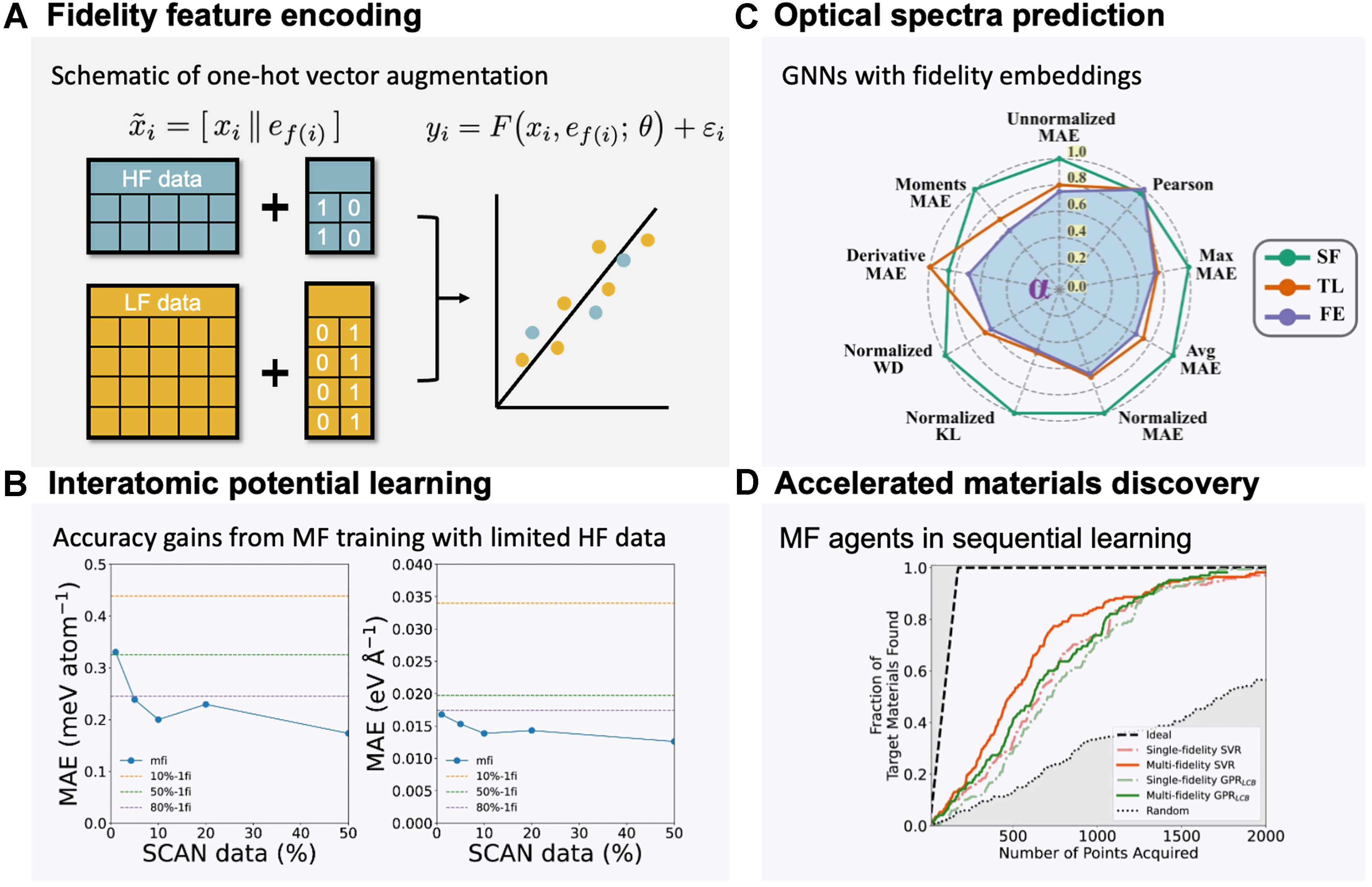
Figure 2. Examples of direct MF learning with fidelity features. (A) Schematic of the one-hot encoding fidelity approach: each sample is augmented with a fidelity indicator vector e _f, allowing a single unified model to learn across low- and high-fidelity data; (B) Interatomic potential for water: test MAEs of a mfi trained with varying fractions of HF (SCAN) data (left: energy; right: force). Dashed lines indicate the MAEs of 1fi baselines using the same fractions of HF data, highlighting the efficiency of MF learning^[39]; (C) Frequency-dependent optical spectra (reduced absorption coefficient α): radar charts show normalized median errors on the HF test set for three GNNs-SF, TL, and FE, demonstrating the performance gains from fidelity-aware embeddings^[66]; (D) Simulated inorganic materials discovery under sequential learning: the x-axis shows the experimental acquisition budget, and the y-axis shows the fraction of ideal materials (with visible-spectrum band gaps) discovered. MF agents with fidelity indicators accelerate discovery relative to SF agents^[47]. MF: Multi-fidelity; HF: high fidelity; LF: low fidelity; MAE: mean absolute error; mfi: multi-fidelity model; 1fi: single-fidelity model; SCAN: strongly constrained and appropriately normed (density functional); GNNs: graph neural networks; SF: single fidelity; TL: transfer learning; FE: fidelity embedding.