

Optimal consensus control of Markov jump multi-agent systems under switching topology
 0
Graphical Abstract
Abstract
This paper investigates the optimal consensus control problem for multi-agent systems with Markov jump characteristics in system parameters and subject to Markov switching in communication topology. Firstly, the cost function is constructed to characterize the impact of topology switching and jumps in system parameters on system performance. Then, to tackle the impact of neighbor coupling terms on the performance of the cost function, the global algebraic Riccati equation is derived to determine the optimal control policy. Within the adaptive dynamic programming framework, global form policy iteration and value iteration algorithm are proposed to solve the global control policy. Subsequently, the convergence of the proposed iterative algorithm is theoretically proved, and the stability of the system is established through the Lyapunov stability theorem. Finally, the effectiveness of the presented optimal control scheme is verified through simulation examples.
Keywords


 Download PDF
1. INTRODUCTION
In recent years, distributed collaborative control for multi-agent systems (MASs) has attracted extensive attention in control theory and industrial engineering[1,2]. MASs consist of multiple nodes that coordinate to accomplish complex tasks[3,4]. Consensus control is a fundamental problem in this field. Its main objective is to design distributed control protocols based on local neighborhood information[5-7]. The literature[7] investigated efficient communication consensus in nonlinear MASs and proposed an adaptive temporal partitioning method to reduce unnecessary information exchange while maintaining consensus performance. Distributed consensus control has been extensively implemented in various practical scenarios, such as unmanned aerial vehicle (UAV) swarm formation, smart grid synchronization, and autonomous industrial manufacturing[8,9]. Since resource allocation must be considered during task execution[10,11], the research focus on MASs has increasingly shifted toward optimal consensus control[12,13]. Specifically, a cost function is constructed and minimized to achieve optimal control. This approach ensures task execution while reducing energy consumption[13].
Physical events such as actuator degradation, sudden payload variations, and unexpected failures frequently cause random transitions within the internal dynamic parameters of the agents. Markov jump systems provide a mathematical framework to describe these structural variations. In this framework, a Markov chain dictates the transitions among different operational modes[14,15]. Recently, Markov jump systems have attracted widespread attention, and numerous results have been reported for both single systems[16,17] and MASs[18,19]. Specifically, the literature[17] focused on fault detection in fuzzy Markov switching systems and proposed an adaptive memory-triggering mechanism to overcome the limitation on communication resources. For MASs, interference attenuation and bump suppression were achieved in[19] by constructing a cost function and an error-state cost, and a balance between stability and performance of bumpless transfer control was achieved using a weighted optimization criterion. In practice, MASs are subject not only to parameter jumps but also to frequently experience changes in their communication topologies due to external environmental factors[20,21]. Consequently, MASs with switching topology have been extensively studied[22,23]. For example, the consensus problem for MASs with Markov switching topology and time-varying delays was investigated in[22], where necessary and sufficient consensus conditions were established by considering stochastic noises and two types of network-induced delays. In[23], the scholars transformed a time-delay system into a delay-free system by introducing state variables and designed a value iteration (VI) algorithm according to the inputs and outputs of the system to solve the consensus problem for MASs. Notably, most existing studies focus solely on jumping parameters in single systems or switching topology in MASs. However, current research on consensus issues in MASs under sudden changes in system parameters and communication topology switching is insufficient, which motivated the work presented in this paper.
On the other hand, practical systems must not only ensure stability during task execution but also optimize their operational costs. Consequently, optimal control problems have attracted significant attention for both single systems[24,25] and MASs[26,27]. Specifically, a novel quasi-model network was developed in[24] to solve the problem of system model pretraining, and an algorithm based on the adaptive dynamic programming (ADP) method was developed to address the optimal control problem for unknown continuous-time affine systems. Meanwhile, the literature[26] designed an optimal consensus control scheme for MASs based on the Hamilton-Jacobi-Bellman (HJB) equation and proposed a novel policy iteration (PI) algorithm for online learning of the solution of the HJB equation. At present, the core of most methods for solving optimal consensus problems is to derive a coupled HJB equation. However, obtaining analytical solutions is difficult due to factors such as the nonlinearity of the cost function kernel matrix. To overcome this challenge, various ADP-based PI[28,29] and VI[30,31] algorithms have been proposed to approximate the solutions of the HJB equation. For example, an iterative policy based on an adaptive evaluator was used in[29] to find the state-feedback, infinite-horizon optimal control solution for linear continuous-time systems, and this algorithm converges to the optimal control solution without requiring an explicit, pre-determined model of the system’s internal dynamics. The literature[30] solved the linear quadratic regulator problem using the VI algorithm and proposed a discounted cost function to achieve optimal control. However, these studies overlook the impact of neighbor coupling terms (NCTs) on system performance. Therefore, an improved ADP method is required to address the issue of NCTs, which raises two questions. (1) How to design an improved ADP method to avoid interference from NCTs? (2) How to design suitable PI and VI algorithms to derive the optimal control policy? This motivated the work presented in this paper.
Based on the previous discussion, the optimal consensus control problem of MASs satisfying both Markov jump dynamics and Markov-switching topology is solved through the ADP approach. The main novelties and contributions are summarized as follows.
• The existing studies[16,23] investigated the optimal control problem for single or multiple systems subject to jumping system parameters or communication topologies. In this paper, the problem of optimal consensus for MASs involving jumping parameters and switching topologies is discussed. Then, a cost function is formulated to evaluate the impact of these two types of switching on system performance.
• Unlike[32], the algebraic Riccati equation (ARE) cannot be successfully derived due to the influence of NCTs. This paper derives a global ARE to solve the optimal control policy under the influence of NCTs. Based on the ADP framework, we develop global policy iteration (GPI) and global value iteration (GVI) algorithms to approximate the controller gain.
The remainder of this paper is structured as follows. Section 2 shows the problem formulation and preliminaries. GPI and GVI algorithms are proposed to find optimal control policy, with the convergence of the algorithms and the stability of the system analyzed in Section 3. The validity of the theoretical results obtained through numerical simulation was verified in Section 4. Finally, Section 5 summarizes the work presented in this paper.
2. PROBLEM FORMULATION AND PRELIMINARIES
2.1. Notation
The symbol
2.2. Graph theory
Define a directed graph
For a time-variant topology, the dynamic communication structure at time step k is
Assumption 1 Under the framework of Markov switching topology, the associated union graph is assumed to contain a directed spanning tree, with the switching signal
2.3. Problem formulation
Consider MASs consisting of one leader and N followers. The dynamic evolution equations for each follower and the leader can be expressed as follows:
where xi(k) ∈ ℝn is the state of the i-th agent, x0(k) ∈ ℝn is the state of the leader and ui(k) ∈ ℝm denotes the system input. g represents a simplified symbol for a Markov chain {g(k)}, which takes values in a finite set
The transition probability of the Markov chain{g(k)} is defined as
where πgp is the transition probability from mode g to mode p at the next time step with πgp ≥ 0 for all g, p ∈ S and Σp=1mπgp = 1 for each mode g.
Denote the tracking error of the local neighborhood for the i-th agent by
Then, the dynamic evolution equation for the error system of agent i is expressed as follows:
Remark 1 It is worth noting that both Ag and Bg depend on the Markov jump process g(k), while aijℓ, biℓ, and liiℓ rely on the switching signal
To characterize the cost of the agent, the cost function of the i-th agent in mode g is defined as follows:
where Qig is the semidefinite matrix and Rig is the positive definite matrix.
Remark 2 In the cost function (5), the utility function Cig of each agent consists of two components: the tracking error (3) and the energy consumed by the control input ui(k). This paper aims to make all followers reach consensus with the leader and minimize the cost function (5) of agent i at the same time. To achieve the optimization goal of the system, it is crucial to select appropriate weight parameters in the utility function Cig. According to the classical linear quadratic regulator theory[33], the weighting matrix Qig directly affects the convergence rate of the system states, while Rig is closely related to the control input energy. Therefore, practical implementation requires a reasonable balance between system energy consumption and convergence performance.
Based on the above analysis, the main objective of this paper is to design an optimal controller ui(k) that enables the MASs to achieve optimal consensus.
2.4. Problem transformation
In order to solve the optimal control problem in Markov jump MASs, a cost function is defined for each agent under different modes in Equation (5). Since mode jumps can affect system performance and complicate the stability analysis, the cost function is reformulated. Meanwhile, the optimal control policy is difficult to express in a linear state-feedback form due to the NCTs. For this reason, the method of restructuring the cost function is adopted to settle the problem caused by the jumping parameter. Subsequently, a global approach is proposed to address the interference caused by NCTs.
Inspired by[16], the transition probability (2) is utilized to reconstruct the cost function for each agent, as shown below:
Hence, the control problem for MASs is formulated as a multiobjective optimization problem. The above multi-objective problem is transformed into a single-objective problem by employing the weighted sum method. The reconstructed cost function is written as
where λg > 0 is a weight coefficient and Σg=1mλg = 1. λg represents the weights associated with the system parameter modes. Its values can be generated by using the transition probabilities πgp between system modes. Moreover, in practice, users can influence system performance by adjusting λg.
With the Equations (6) and (7), the cost function of each agent is derived as follows:
where Dg = Σp=1mλpπpg > 0. cig(ei(k), ui(k)) = ei(k)T
Due to the interference from the NCTs, it is difficult to directly establish a linear relationship between the controller ui(k) and the tracking error ei(k). To overcome this limitation, the global forms of the controller and error are proposed to establish a linear relationship between the controller and the error system.
The global error vector E(k) and the global control vector U(k) are defined as
From the Equation (4), the dynamic evolution equation of the global error system is established as follows:
where
3. OPTIMAL CONSENSUS CONTROL FOR MASS UNDER SWITCHING TOPOLOGY
In this section, a global cost function is derived to solve the problem of interference from NCTs in the derivation of the optimal control policy. Then, the optimization problem is converted into a minimization problem in mathematics using Bellman’s optimality principle. Based on this, GPI and GVI algorithms are developed to find the optimal control policy. Finally, the monotonicity of the cost function kernel matrix is derived to prove the convergence of the algorithm, and the Lyapunov stability theorem is applied to verify the system’s stability.
3.1. Optimal consensus control
From the Equations (8) and (9), the global cost function is derived as below:
where the matrix Q, the matrix R, and the global kernel matrix P are expressed as follows:
where the matrix Pii is the kernel matrix of the cost function Vi(ei(k)) and is the positive definite matrix. Since the cost function can be expressed in a quadratic form V(E(k)) = ET(k)PE(k), Equation (11) is rewritten as
By Bellman’s optimality principle, the optimal cost function V*(E(k)) is defined as
Then, the Hamilton function is constructed as follows:
Moreover, the first-order necessary condition requires that
where
Remark 3 The researchers in[23,28,34] derived the corresponding Hamilton function by constructing a cost function for each agent and determined the optimal control policy. A local neighborhood tracking error system is established. It is worth noting that, due to the influence of the NCTs, the methods of[23,28,34] cannot derive the ARE based on the local cost function, which makes it difficult to derive the optimal control policy. To this end, a global cost function is developed to derive the global ARE in this paper. Subsequently, GPI and GVI algorithms are proposed to obtain approximate solutions for the global ARE and thereby determine the optimal controller. Compared with the aforementioned literature, the GPI and GVI algorithms developed in this paper are intended to address the problem that the ARE cannot be established due to NCTs. In addition, since matrix P in Equation (17) exhibits nonlinear characteristics, its exact solution is difficult to obtain.
Remark 4 The problem of optimal consensus control of MASs is considered in[28], where the optimal control policy is derived as ui*(k) = -
Notably, the above equation contains the term
3.2. GPI algorithm and GVI algorithm
To calculate the solution of the global ARE, GPI and GVI algorithms are proposed below. Proofs of the convergence of the two algorithms will be provided in Section 3.3.
Combining the Equations (13) and (16), the Lyapunov equation is given by
Definition 1 (Admissible Control) If there exists a control policy U(k) that ensures the cost function (11) is bounded and makes the system (10) stable, then this policy is an admissible control.
The specific implementation details of the proposed GPI and GVI algorithms are detailed in Algorithm 1 and Algorithm 2, respectively.
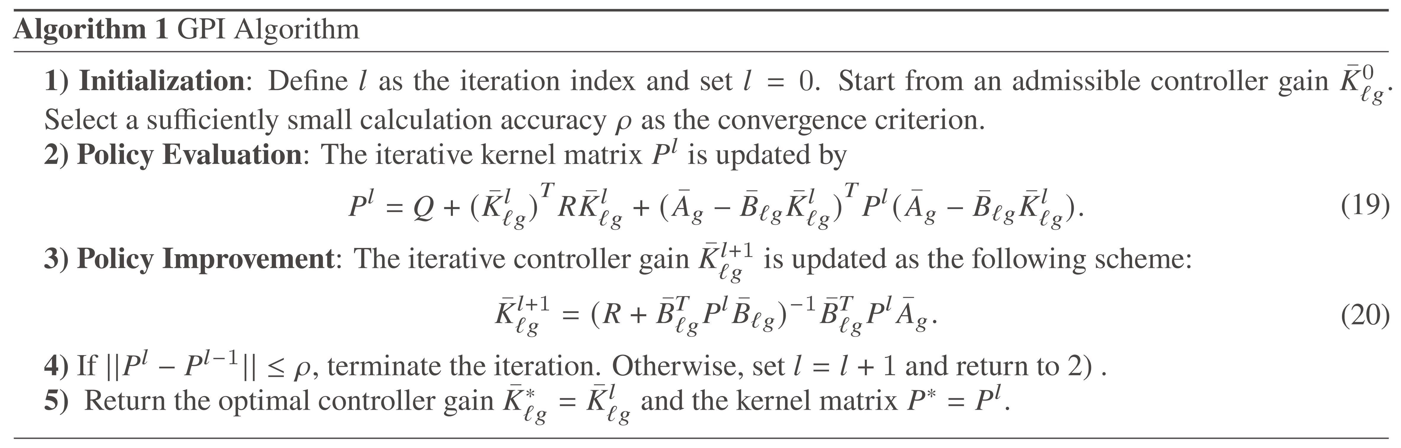
Algorithm 1.
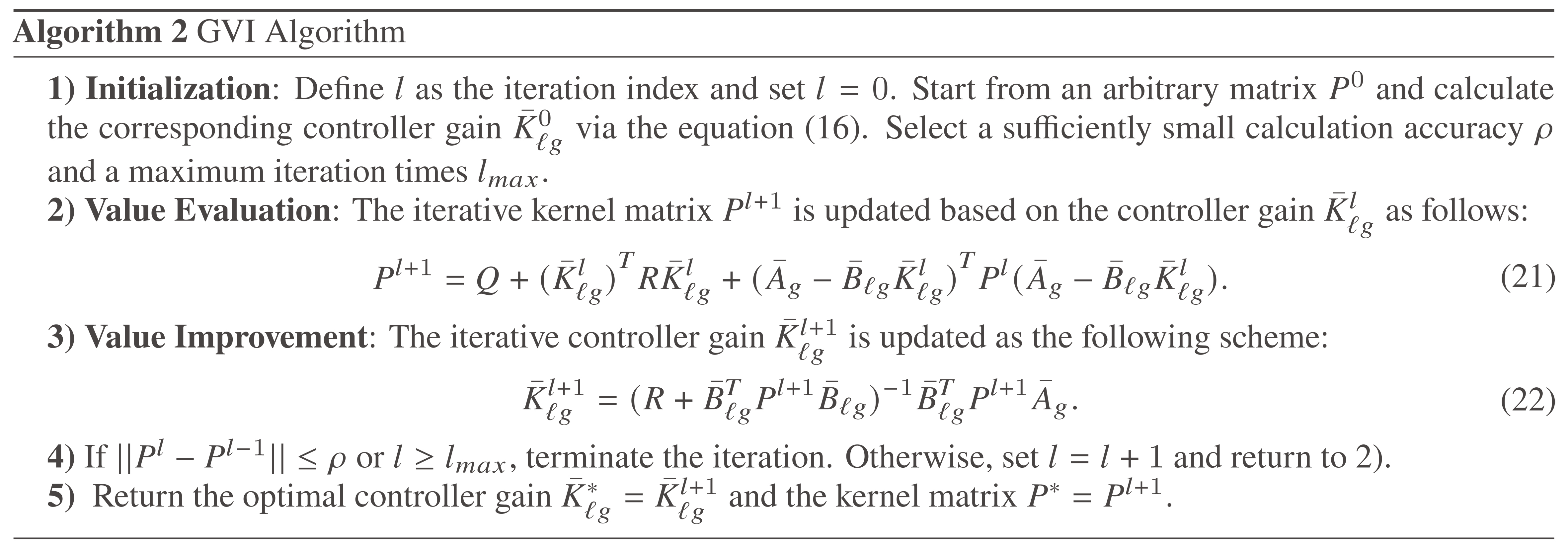
Algorithm 2.
Since the GPI algorithm requires the prior determination of an admissible policy, it exhibits a certain degree of conservatism. In comparison, the VI algorithm allows the utilization of any initial policy. Hence, the following algorithm is designed to solve for an approximate solution of ARE.
Remark 5 In contrast to traditional local controller ui*(k) = -(Ri + BiTPiBi)-1BiTPi*Aiei(k), the global optimal controller is provided in the Equation (16). The reason is that it is difficult for traditional local controllers to utilize the ARE approach for solving the optimal controller, whereas the global controller in (16) mitigates the influence of NCTs. In fact, the controller ui(k) of each agent can also be derived in this paper: ui(k) = -Kiiei(k) - Σj=1NKijej(k), where Kii = (liiℓ + biℓ)[
3.3. Properties of iterative algorithms and stability of system
This subsection analyzes the algorithms’ monotonicity and determines their convergence properties. Then, the proof of the stability for the closed-loop system is given.
Lemma 1 The iterative cost function Vl(E(k)) of GPI is a monotonically nonincreasing sequence, that is, the following relationship holds: Vl+1(E(k)) ≤ Vl(E(k)).
Proof The matrix ψl is designed to be
Hence, the Equation (19) can be written as
A function of a matrix is defined as follows:
According to Equation (16), the following conclusion can be drawn:
A matrix
• Assuming that K =
• When K is the gain of any controller, the following condition is true:
Due to the relationship that
Therefore, it can be concluded that: Pl
Lemma 2 Define the iterative cost function Vl of GVI as
If the kernel matrix Pl+1 and controller gain
• If P1 - P0
• If P1 - P0
Proof It is first demonstrated that the cost function sequence is nondecreasing under the assumption P1 - P0
Due to P1 - P0
which means
Assuming that Vl(E(k)) ≥ γl-1(E(k)) is true, it follows that Vl(E(k+1)) ≥ γl-1(E(k+1)) holds. Considering
which indicates
Based on the Equation (21), a function is given by
Select the matrix M as the kernel matrix of the Equation (30), the following equation holds: γl(E(k)) = ET(k)MlE(k). By the conditions defined above, one can conclude that: M0 = P0. Subsequently, assume that the relationship between Ml and Pl satisfies Ml
From the Equation (21) and the Equation (36), the following conclusion is obtained: Ml+1
Then, the following conclusion can be derived:
which implies
Hence, the first part of the proof is completed by mathematical induction.
Next, prove that the sequence of the cost function is nonincreasing by assuming P1 - P0
Due to P1 - P0
which yields
Assuming that Γl(E(k)) ≤ Vl-1(E(k)) is true, it follows that Γl(E(k+1)) ≤ Vl-1(E(k+1)) holds.
Considering the following equation:
which means
The proof of Γl+1(E(k)) ≥ Vl+1(E(k)) is similar to the proof given above and will not be repeated here. Then, the inequality can be represented as
Therefore, the second part is proven to be complete using mathematical induction.
Remark 6 In[30], the monotonicity of the VI algorithm is proved by constructing two specific functions and comparing them with the cost function, but a complete proof of γl(E(k)) ≥ Vl(E(k)) is not provided. A rigorous proof of this inequality is given in Lemma 2 of this paper. The proof shows that the monotone property of the cost function relies on the comparison between P1 and P0. Once this relationship is established, the monotonic behavior is preserved throughout the iterations.
Theorem 1 Suppose the sequences
Proof Since the iterative cost function in Algorithm 1 and the iterative cost function in Algorithm 2 when P1 - P0
As the matrix sequence {Pl} is monotonically bounded, there exists a limit liml→∞ Pl =
As a result, the limit matrix
Next, the convergence of the iterative kernel matrix Pl in Algorithm 2 when P1 - P0
where γ0(E(k + l + 1)) = 0. Thus, the inequality is shown from (45) as follows:
By the Equation (37), it follows that Vl+1(E(k)) ≤ γl+1(E(k)) ≤
Theorem 2 Assuming that the U*(k) is provided by the Equation (16) and V*(E(k)) complies with the Equation (14), then the system (10) converges to an asymptotically stable state, and the consensus of the agents is reached.
Proof Select optimal cost function V*(E(k)) as a Lyapunov function, whose specific form as
where Q
Furthermore, from the inequality
From Equations (10), (16), and (23), the difference of the Lyapunov function is defined as
In particular, the above conditions imply that
Combining Equation (51) and the Lyapunov stability theorem, the state of the error system (10) is asymptotically stable.
4. SIMULATION EXAMPLES
This section verifies the developed algorithms and the designed controller through two simulation examples. In particular, Example 1 demonstrates the numerical simulation and compares it with methods in the existing literature. Then, Example 2 validates the effectiveness of the proposed approach in practical systems.
Example 1: Consider a MAS consisting of one leader and six followers. Specifically, the system matrices are shown by
Thereafter, the transition probability (2) is chosen in matrix form as [πgp]2×2 =
Select an appropriate stationary distribution χ > 0 to ensure the ergodicity of the Markov parameter jump process. Correspondingly, the transition probability matrix for the topology switching process
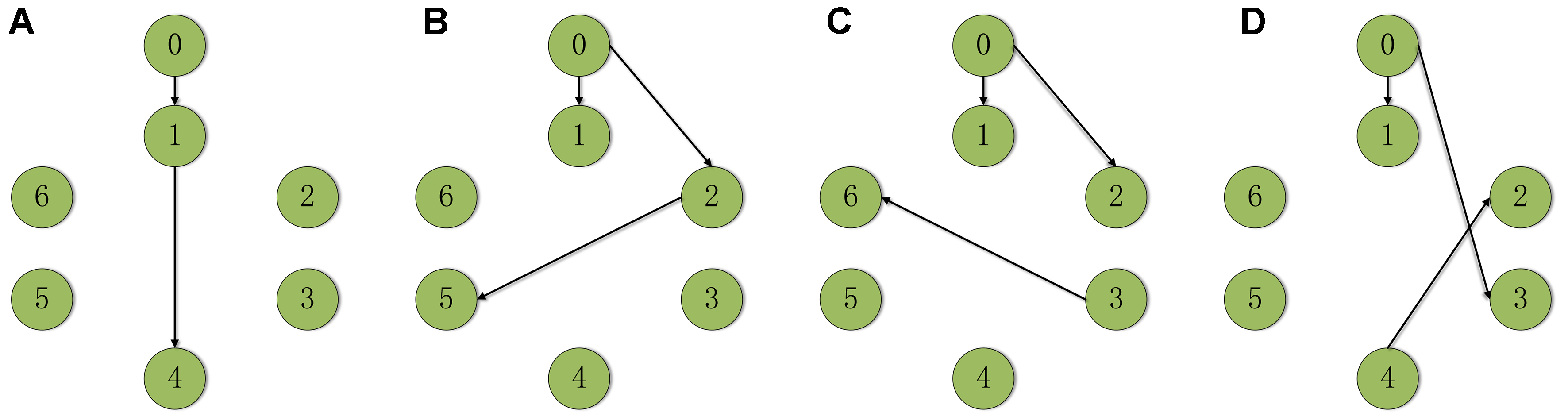
Figure 1. Switch topology diagram.
The 3D diagram in Figure 2 presents the trajectories of all agents, while Figure 3 displays the state curves for each agent. Figure 4 shows the curves of the norms of the local tracking error ei(k) and the global tracking error E(k). From Figures 2-4, it can be observed that under the action of the global controller, the states of all follower agents successfully track the dynamic trajectory of the leader, and the local and global tracking errors converge to 0 in approximately 8 s. This indicates that leader-follower consensus has been achieved and demonstrates the validity of the proposed control policy.
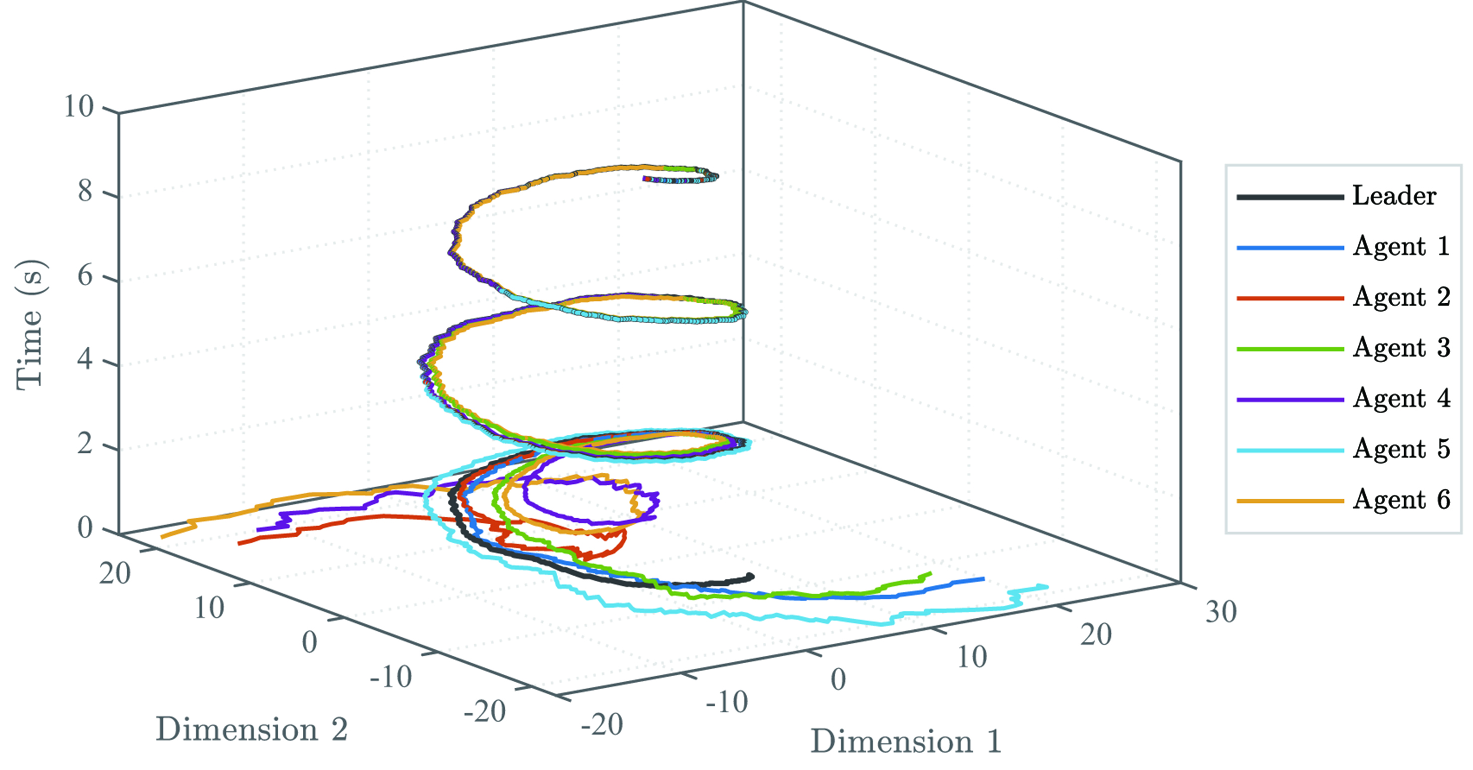
Figure 2. 3D diagram of system states under Markov jump of the parameter and Markov switching topology.
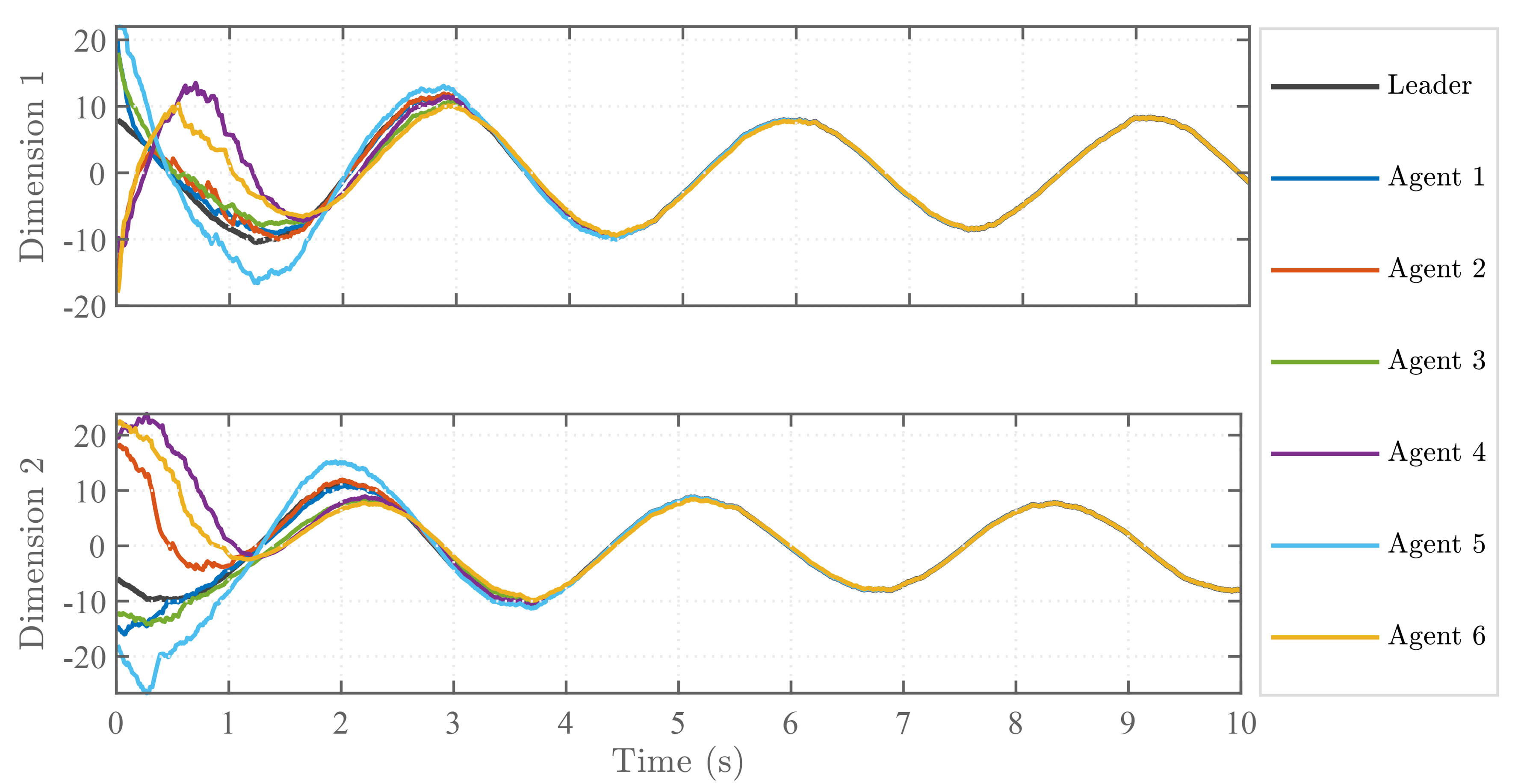
Figure 3. The state curve of each agent under the optimal controller.
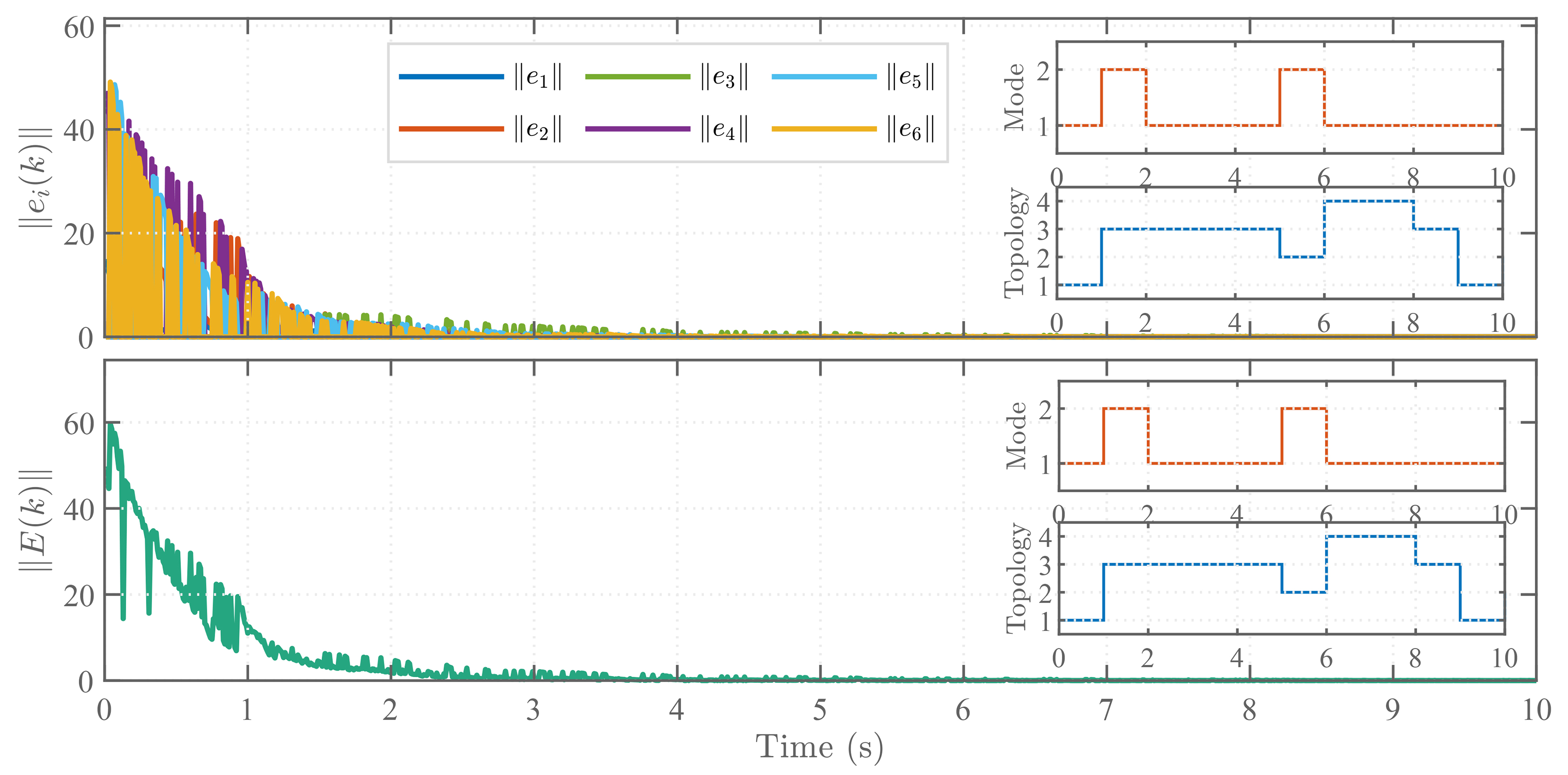
Figure 4. The norms of ei(k) and E(k) under jumping signals g(k) and
Figures 5 and 6 plot the curve of the norm of the kernel matrix Pl and the norm of the control gain matrix
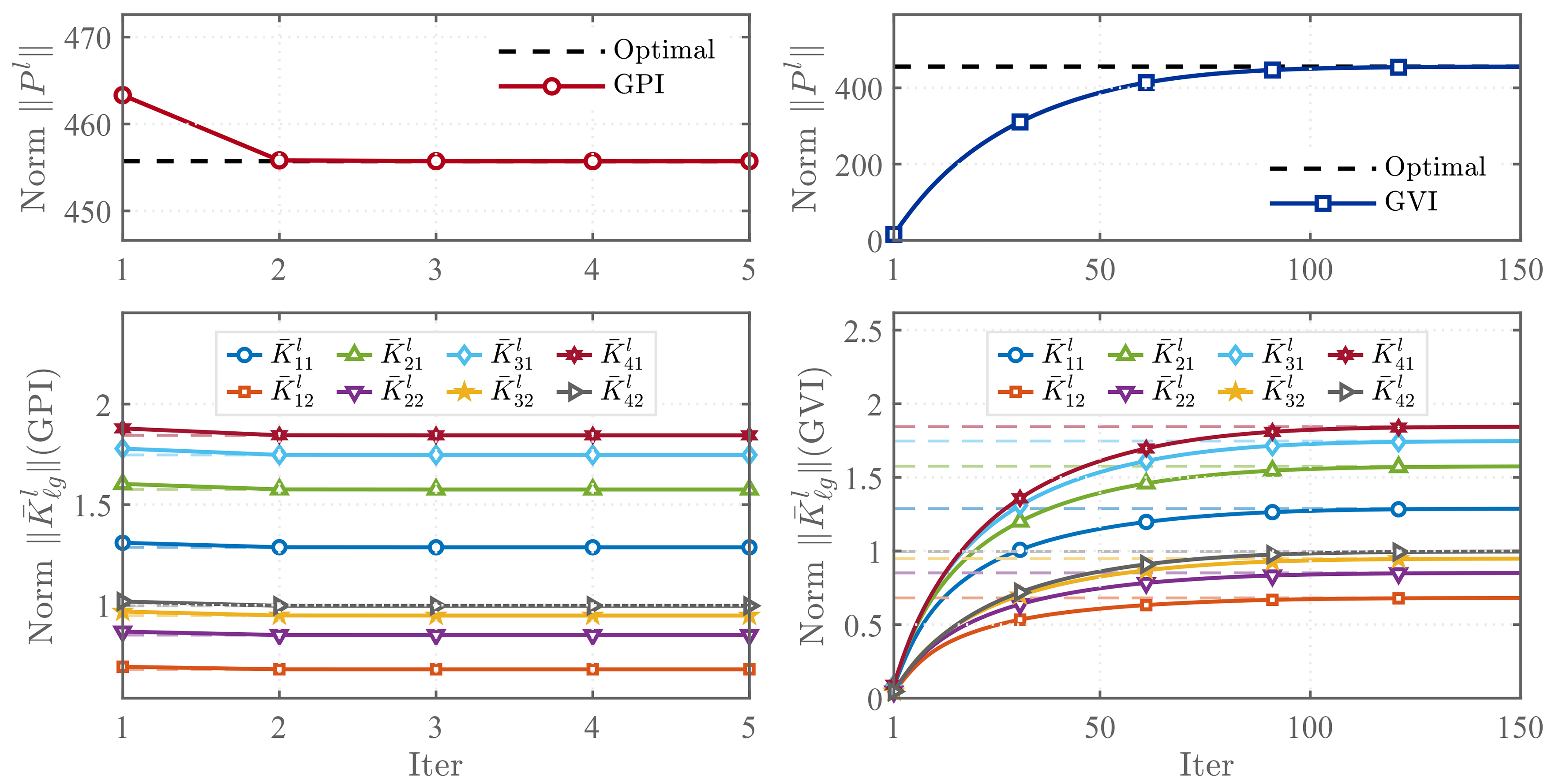
Figure 5. Convergence of GPI and GVI algorithms. GPI: Global policy iteration; GVI: global value iteration.
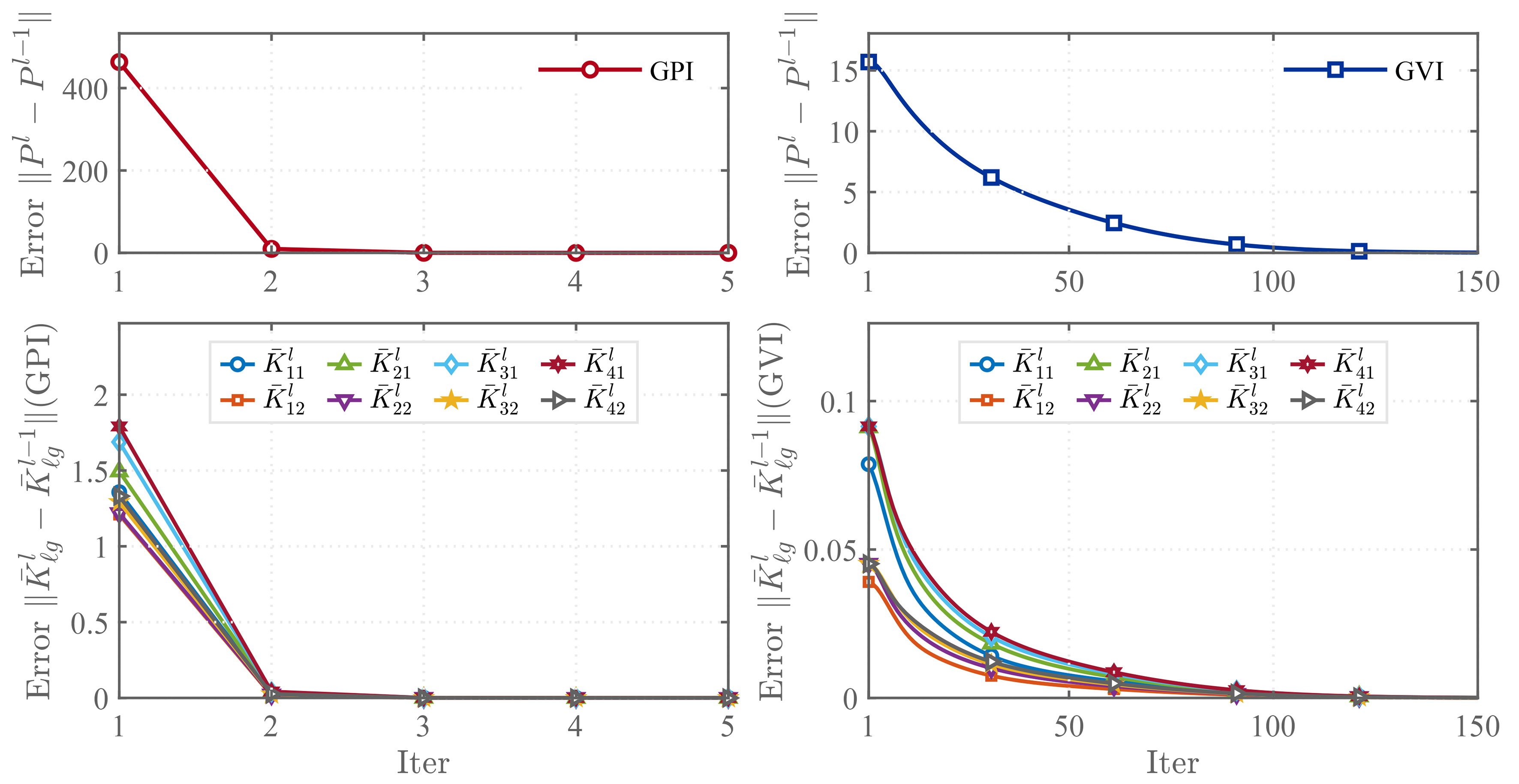
Figure 6. Iterative error in GPI and GVI algorithms. GPI: Global policy iteration; GVI: global value iteration.
Table 1 compares the characteristics of the presented approach in this paper with those of existing studies[16,23,28]. It should be noted that × indicates that the literature considers NCTs in the system, but the influence of NCTs cannot be eliminated through the ARE framework, making it impossible to derive the optimal controller. By contrast, √ denotes the case where the literature considers NCTs in the system, but the influence of NCTs can be eliminated through the ARE framework. Prior research has proposed several algorithms for finding approximate solutions to the optimal controller. Nevertheless, the optimal consensus problem for Markov jumping parameter under the Markov switching topology has not been thoroughly investigated. Specifically, the literature[16] studied the stability of Markov jumping parameter systems, while the literature[23] investigated the optimal consensus of MASs under a Markov switching topology. In this paper, GPI and GVI algorithms are proposed to successfully calculate an approximate solution for the optimal controller in both of these cases. Notably, the methods in[23,28] are affected by NCTs when solving for the ARE. Thus, they are unable to successfully derive the ARE, and the optimal control policy cannot be computed. The global ARE using the global method is successfully derived in this paper. Based on this, two global algorithms are proposed for approximating the optimal control policy.
Comparison with literature
Then, Table 2 describes the consensus comparison between this paper and the literature[23,35,36] under Markov jumping parameter and Markov switching topology, as well as the optimality comparison under the ARE framework. In contrast, although the method employed in the literature[23] achieves consensus under Markov jumping parameter and Markov switching topology, it fails to achieve optimality within the ARE framework. Meanwhile, the methods used in the literature[35,36] cannot achieve consensus under Markov jumping parameter and Markov switching topology. By comparison, the method proposed in this paper achieves optimal consensus within the ARE framework. This further verifies that the proposed approach effectively resolves problems that have not been sufficiently investigated in earlier literature.
Performance comparison under Markov jumping parameter and Markov switching topology
Subsequently, as shown in Figures 7 and 8, a comparison is conducted between the proposed algorithm and the VI algorithm based on gradient and neural network approximation presented in the literature[23], subject to both Markov jumping parameter and Markov switching topology. Correspondingly, the convergence number of ||Piil|| and the norm of the tracking error for each agent under the two algorithms are compared using identical parameter settings and illustrated in Figures 7 and 8. As shown in Figures 7 and 8, the algorithm proposed in this paper can mitigate the effects of NCTs while ensuring comparable performance to the VI algorithm in[23].
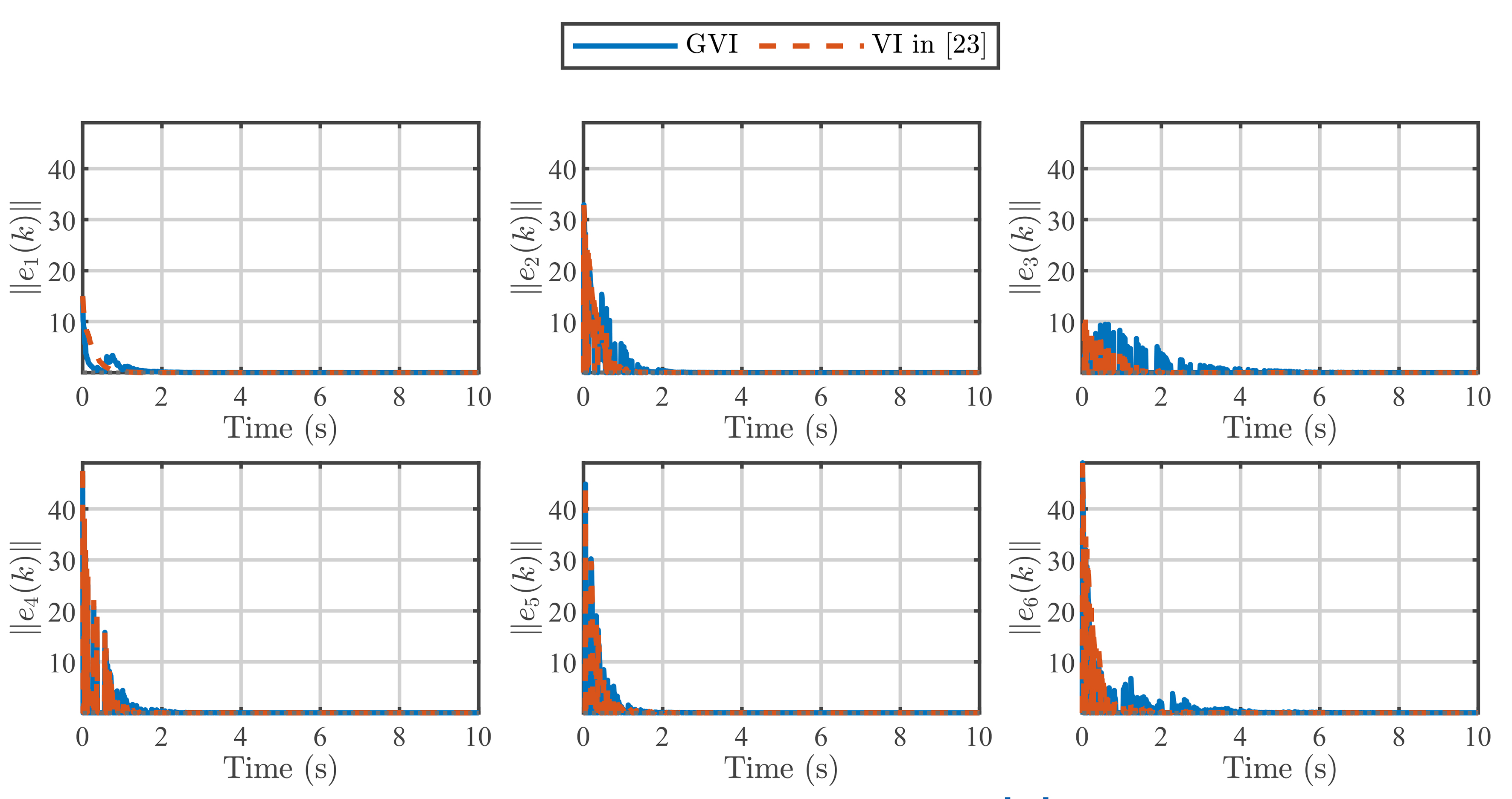
Figure 7. The norm of the tracking error for each agent under VI in[23] and GVI. VI: Value iteration; GVI: global value iteration.
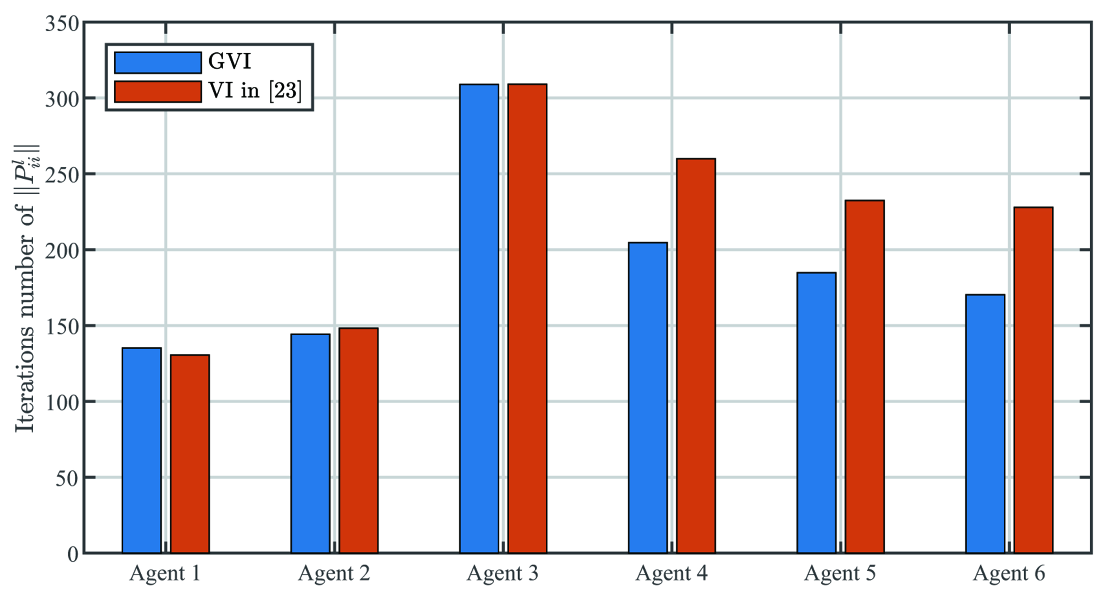
Figure 8. Iterations number of ||Pil||.
Example 2: To further demonstrate the effectiveness of the proposed optimal consensus control method in practical applications, this example applies a practical example related to UAVs[37,38]. According to the literature[37] and[38], the dynamics of the agent represented by a UAV can be expressed as
where
The jump between the two UAV modes is governed by the Markov chain g(k), whose transition probability matrix is chosen as [πpq]2×2 =
This paper employs the switching topology to describe the exchange of information among agents. Figure 9 shows the switching topology diagram and the joint connect diagram. The transition probability matrix for the topology switching signal
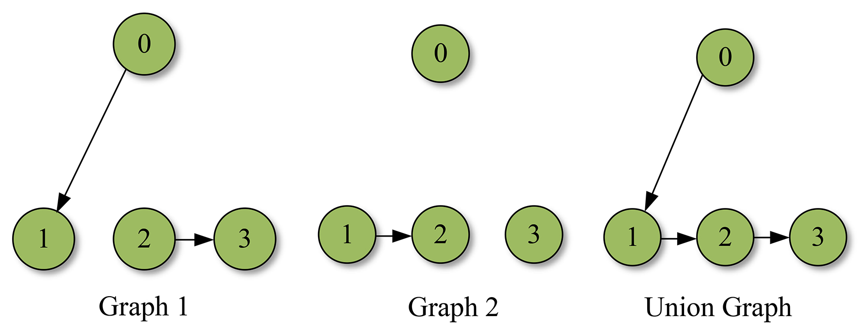
Figure 9. The switching topology graph.
The initial states of one leader agent and three follower agents are as follows: x0(0) = [-2, 4]T, x1(0) = [0, 3]T, x2(0) =[2, 2]T, x3(0) = [4, 1]T by choosing suitable si and ri, i = 0, 1, …, N. Using the optimal controller (16), the tracking error of local neighborhood and the global error system are depicted in Figures 10 and 11, respectively. Subsequently, Figure 12 illustrates the convergence of the GPI and GVI algorithms. From the simulation results, it can be found that both algorithms converge as the number of iterations increases.
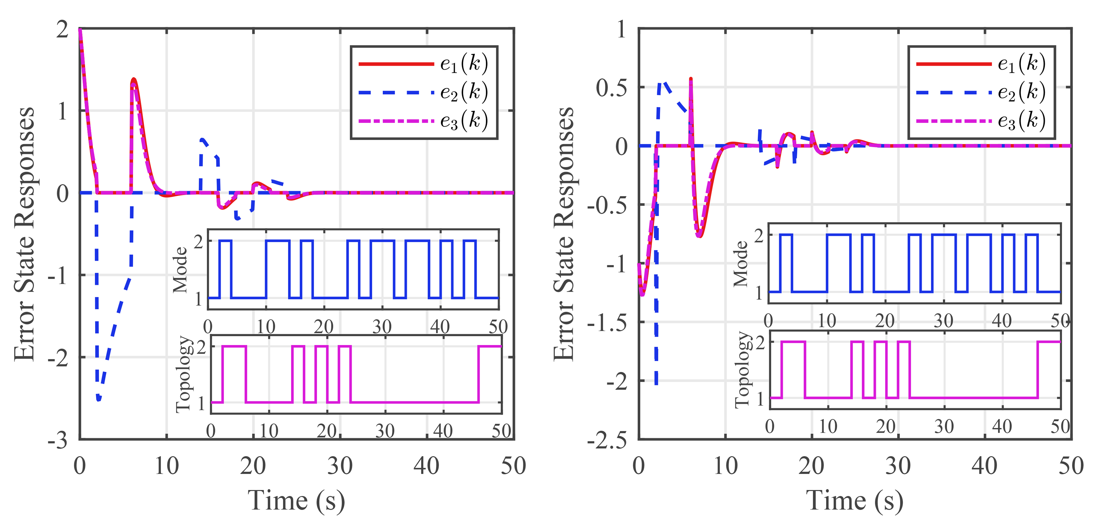
Figure 10. The local tracking error ei(k) under jumping signals g(k) and
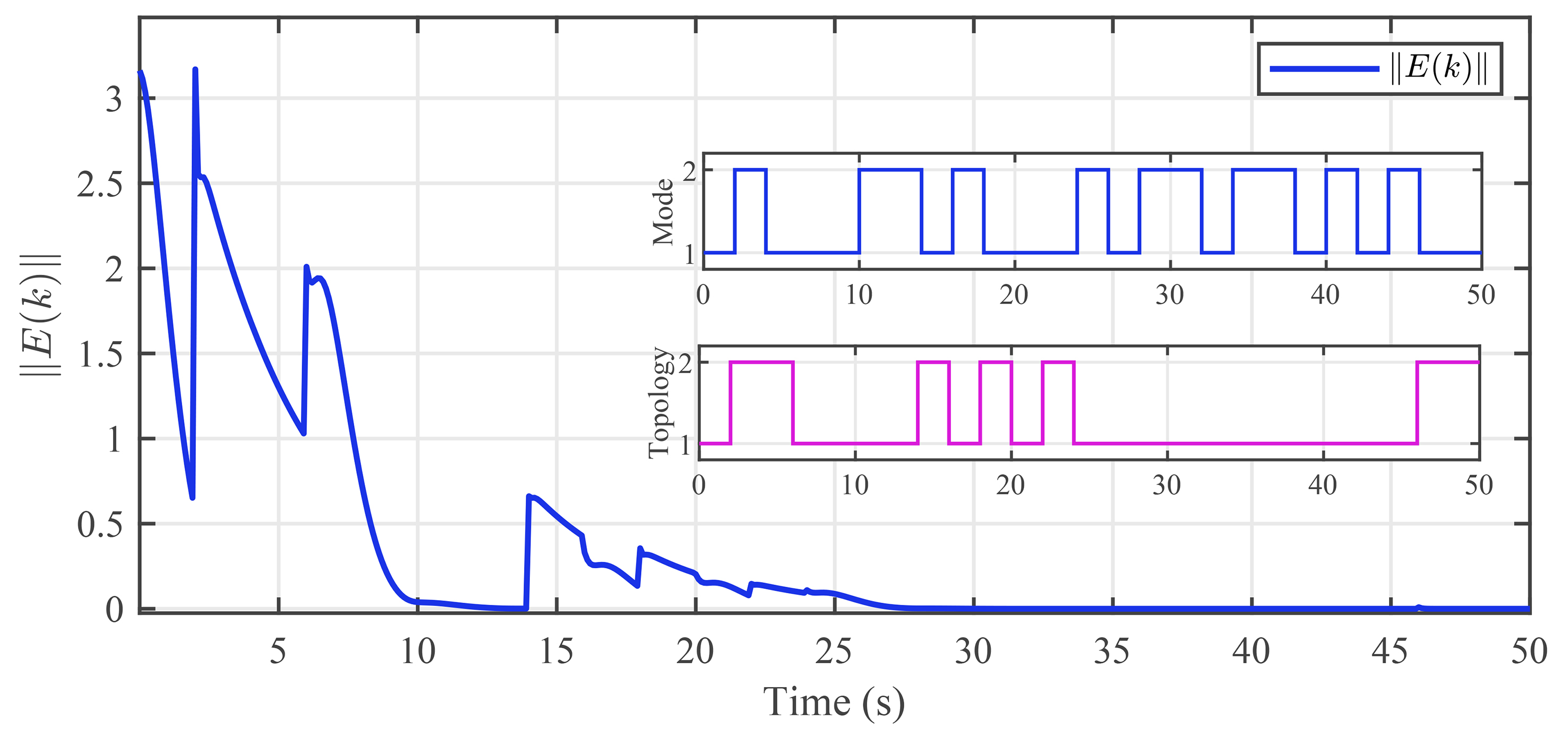
Figure 11. The Norm of global tracking error E(k) under jumping signals g(k) and
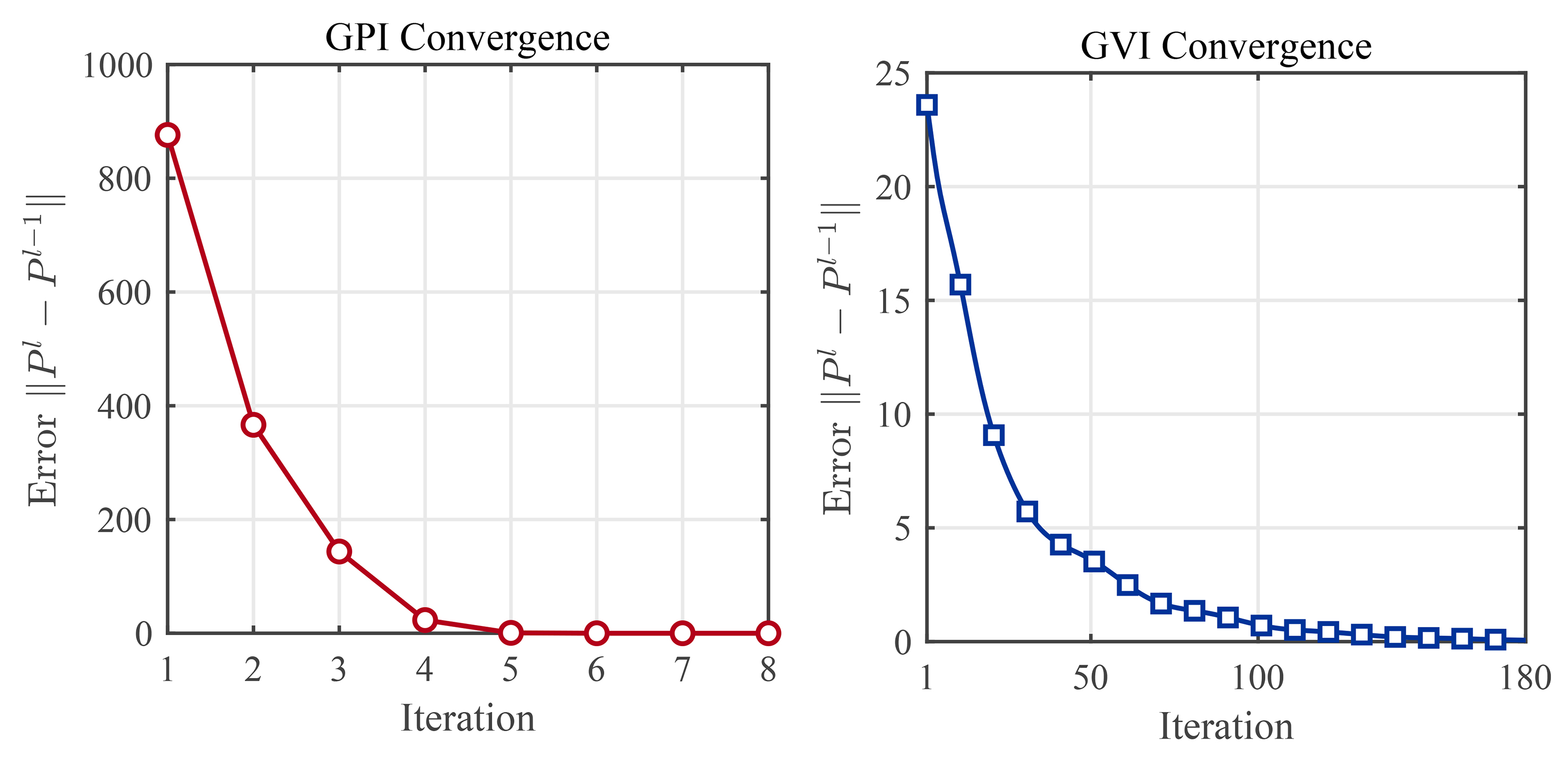
Figure 12. Iterative errors of GPI and GVI algorithms. GPI: Global policy iteration; GVI: global value iteration.
Through the simulation example, the state curves of the leader and each follower are obtained and are shown in Figure 13. As can be seen from the figure, under the designed consensus control policy, the followers always reach consensus with the leader agent.
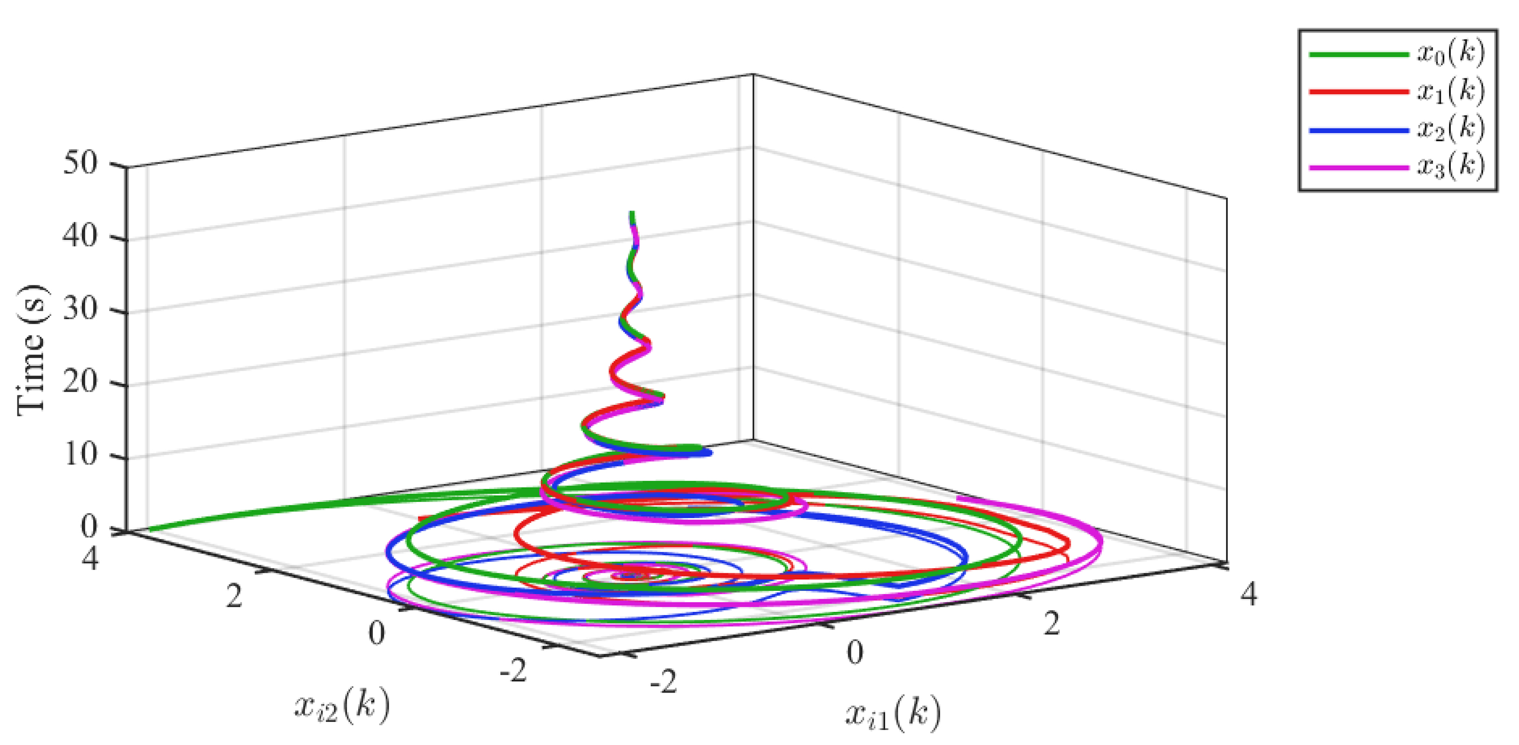
Figure 13. The state curves of all agents in the 3D plane.
5. CONCLUSION
The problem of optimal control for MASs with Markov jumping parameter under the Markov switching topology has been investigated. Since optimizing the analysis becomes complicated when defining a cost function for each agent in each mode, the cost function restructuring approach has been employed. Then, a global cost function is constructed to alleviate the influence of NCTs on the system performance and the global ARE is derived. Based on this, GPI and GVI algorithms inspired by ADP framework are proposed to approximate the optimal controller gain. Subsequently, the convergence of the algorithms and the stability of the system have been proven. Finally, simulations demonstrate that the proposed control policy and algorithms achieve comparable performance to reported in the existing literature and mitigate the impact of NCTs, while ensuring optimal consensus under Markov jumping parameter and Markov switching topology.
In future research, the topic of optimal consensus in heterogeneous MASs is of great significance. The issue of interdependence between two Markov jump processes also warrants further study. In addition, the practical system may suffer from cyber attacks (e.g., denial-of-service attacks and false data injection attacks). This means that it is important to study the impact of cyber attacks on the performance of MASs.
DECLARATIONS
Authors’ contributions
Made substantial contributions to mathematical derivations, algorithm design, and simulation, wrote and edited the original manuscript: Liu, B.
Provided key feedback for this study and assisted in the completion of the simulation: Xing, W.
Conceived and proposed this study: Yang, H.
Checked the results and assisted in the improvement of the manuscript: Zhang, J.
Availability of data and materials
All data used to support the findings of this study are presented in the simulation section.
AI and AI-assisted tools statement
Not applicable.
Financial support and sponsorship
This work was supported by National Natural Science Foundation of China (62463007, 62463005, and 62563006), Natural Science Foundation of Hainan (625RC710 and 625MS047), Postdoctoral Research Funding of Hainan Province (2025-79), and Postgraduate Innovative Research Funding of Hainan Province (Hyb2025-22 and Hyb2025-31).
Conflicts of interest
All authors declared that there are no conflicts of interest.
Ethical approval and consent to participate.
Not applicable.
Consent for publication.
Not applicable.
Copyright
© The Author(s) 2026.
REFERENCES
1. Olfati-Saber, R.; Fax, J. A.; Murray, R. M. Consensus and cooperation in networked multi-agent systems. Proc. IEEE. 2007, 95, 215-33.
2. Liang, Z.; Cao, J.; Jiang, S.; Xu, H. Hierarchical reinforcement learning with partner modeling for distributed multi-agent cooperation. IEEE. Trans. Parallel. Distrib. Syst. 2024, 1-13.
3. Peng, C.; Zhang, A.; Li, J. Neuro-adaptive cooperative control for high-order nonlinear multi-agent systems with uncertainties. Int. J. Appl. Math. Comput. Sci. 2021, 31, 635-45.
4. An, R.; Wang, Y.; Zhao, Y.; Zhang, J. Consensus of high-order multiagent systems with binary-valued communications and switching topologies. IEEE. Trans. Control. Netw. Syst. 2025, 12, 1369-80.
5. Li, B.; Zhao, L.; Wen, S. Periodic event-triggered consensus of stochastic multi-agent systems under switching topology. AI. Sci. Eng. 2025, 1, 147-56.
6. He, W.; Chen, X.; Zhang, M.; Sun, Y.; Sekiguchi, A.; She, J. Data-driven optimal consensus control for switching multiagent systems via joint communication graph. IEEE. Trans. Ind. Inf. 2024, 20, 5959-68.
7. Zhang, L.; Li, Y.; Ahn, C. K.; Liang, H. Adaptive temporal partitioning for communication-efficient consensus in nonlinear multiagent systems. IEEE. Trans. Ind. Informat. 2026, 1-12.
8. Jin, N.; Xu, J.; Zhang, H. Distributed optimal consensus control of multiagent systems involving state and control dependent multiplicative noise. IEEE. Trans. Autom. Control. 2023, 68, 7787-94.
9. Wan, X.; Guo, Y.; Wu, X. Differentially private consensus for multi-agent systems under switching topology. IEEE. Trans. Circuits. Syst. II. 2023, 70, 3499-503.
10. Xing, W.; Zhao, X.; Basar, T.; Xia, W. Security investment in cyber-physical systems: stochastic games with asymmetric information and resource-constrained players. IEEE. Trans. Autom. Control. 2022, 67, 5384-91.
11. Yang, C.; Zhang, X.; Zhang, L.; et al. Coordinated energy-efficient walking assistance for paraplegic patients by using the exoskeleton-walker system. Intell. Robot. 2024, 4, 107-24.
12. Yang, A.; Liang, X.; Zhang, J.; Hou, Y.; Wang, N. Global optimal consensus for UAV swarms with time-varying objective functions and bounded input constraints. IEEE. Trans. Aerosp. Electron. Syst. 2024, 60, 3822-36.
13. Jia, C.; Chen, F. Feasibility of optimal formation under multiplicative noise with energy and time constraints. IEEE. Trans. Autom. Sci. Eng. 2025, 22, 18522-30.
14. Shen, H.; Wang, Y.; Wang, J.; Park, J. H. A fuzzy-model-based approach to optimal control for nonlinear Markov jump singularly perturbed systems: a novel integral reinforcement learning scheme. IEEE. Trans. Fuzzy. Syst. 2023, 31, 3734-40.
15. Tao, Y. Y.; Che, W. W.; Wu, Z. G.; Xu, Y.; Dong, S. Asynchronous control of 2-D Markov jump roesser systems with nonideal transition probabilities. IEEE. Trans. Cybern. 2024, 54, 6643-52.
16. Zhong, X.; He, H.; Zhang, H.; Wang, Z. Optimal control for unknown discrete-time nonlinear Markov jump systems using adaptive dynamic programming. IEEE. Trans. Neural. Netw. Learn. Syst. 2014, 25, 2141-55.
17. Feng, L.; Yang, G. Adaptive memory-event-triggered fault detection for interval type-2 fuzzy Markov jump systems with sensor saturation. IEEE. Trans. Fuzzy. Syst. 2024, 32, 2089-101.
18. Wang, X.; Park, J. H.; Yang, H. An improved protocol to consensus of delayed MASs with UNMS and aperiodic DoS cyber-attacks. IEEE. Trans. Netw. Sci. Eng. 2021, 8, 2506-16.
19. Wang, J.; Dong, J. Robust predictive bipartite bumpless control for Markov jump MASs under switching topology: application to rotary-wing air vehicles. IEEE. Trans. Veh. Technol. 2025, 74, 7020-32.
20. Elhamamsy, A.; Aghili, F.; Aghdam, A. G. Connectivity preservation and collision avoidance in multi-agent systems using model predictive control. IEEE. Trans. Netw. Sci. Eng. 2023, 10, 1779-91.
21. Yao, J.; Li, X.; Zhang, Y.; Ji, J.; Ren, G.; Ren, Z. Obstacle avoidance control for unmanned tracked vehicle formation with communication constraints. IEEE. Trans. Autom. Sci. Eng. 2025, 22, 19735-49.
22. Shang, Y. Consensus of noisy multiagent systems with Markovian switching topologies and time-varying delays. Math. Probl. Eng. 2015, 2015, 1-13.
23. Ji, L.; Wang, C.; Zhang, C.; Wang, H.; Li, H. Optimal consensus model-free control for multi-agent systems subject to input delays and switching topologies. Inf. Sci. 2022, 589, 497-515.
24. Han, X.; Zhao, X.; Karimi, H. R.; Wang, D.; Zong, G. Adaptive optimal control for unknown constrained nonlinear systems with a novel quasi-model network. IEEE. Trans. Neural. Netw. Learn. Syst. 2022, 33, 2867-78.
25. Chen, C.; Lewis, F. L.; Li, B. Homotopic policy iteration-based learning design for unknown linear continuous-time systems. Automatica 2022, 138, 110153.
26. Cai, Y.; Zhang, H.; Zhang, K.; Liu, C. Fuzzy adaptive dynamic programming-based optimal leader-following consensus for heterogeneous nonlinear multi-agent systems. Neural. Comput. Appl. 2020, 32, 8763-81.
27. Yang, H.; Zhang, H.; Wang, Z.; Huang, C.; Yan, H. Fault-tolerant optimal consensus for multiagent systems: a fuzzy-based game approach. IEEE. Trans. Aerosp. Electron. Syst. 2024, 60, 6839-52.
28. Peng, Z.; Zhao, Y.; Hu, J.; Ghosh, B. K. Data-driven optimal tracking control of discrete-time multi-agent systems with two-stage policy iteration algorithm. Inf. Sci. 2019, 481, 189-202.
29. Vrabie, D.; Pastravanu, O.; Abu-Khalaf, M.; Lewis, F. Adaptive optimal control for continuous-time linear systems based on policy iteration. Automatica 2009, 45, 477-84.
30. Wang, D.; Ren, J.; Ha, M.; Qiao, J. System stability of learning-based linear optimal control with general discounted value iteration. IEEE. Trans. Neural. Netw. Learn. Syst. 2023, 34, 6504-14.
31. Ren, Y.; Wang, Q.; Duan, Z. Optimal leader-following consensus control of multi-agent systems: a neural network based graphical game approach. IEEE. Trans. Netw. Sci. Eng. 2022, 9, 3590-601.
32. Zhang, H.; Zhang, J.; Yang, G.; Luo, Y. Leader-based optimal coordination control for the consensus problem of multiagent differential games via fuzzy adaptive dynamic programming. IEEE. Trans. Fuzzy. Syst. 2015, 23, 152-63.
34. Zhang, H.; Jiang, H.; Luo, Y.; Xiao, G. Data-driven optimal consensus control for discrete-time multi-agent systems with unknown dynamics using reinforcement learning method. IEEE. Trans. Ind. Electron. 2017, 64, 4091-100.
35. Ding, J.; Sheng, J.; Li, F.; Xu, J.; Ling, Q. Consensus of multi-agent Markovian jump systems under event-triggered control. In 2023 42nd Chinese Control Conference (CCC), Tianjin, China. Jul 24-26, 2023. IEEE; 2023. pp. 5682-6.
36. Yao, Z.; Zhu, Q.; Qin, P.; Luo, M. Homotopic reinforcement learning for distributed consensus control of stochastic Markov jump multi-agent systems. J. Supercomput. 2025, 81, 7885.
37. Michael, N.; Schwager, M.; Kumar, V.; Rus, D. An experimental study of time scales and stability in networked multi-robot systems. In Experimental robotics; Khatib, O.; Kumar, V.; Sukhatme, G.; Eds.; Berlin: Springer Berlin Heidelberg; 2014. pp. 631-43.
Cite This Article
 Open Access
How to Cite
Liu, B.; Xing, W.; Yang, H.; Zhang, J. Optimal consensus control of Markov jump multi-agent systems under switching topology. Intell. Robot. 2026, 6(4), 868-90. https://dx.doi.org/10.20517/ir.2026.38
Download Citation
If you have the appropriate software installed, you can download article citation data to the citation manager of your choice. Simply select your manager software from the list below and click on download.
Export Citation File
Type of Import
Tips on Downloading Citation
Citation Manager File Format
Type of Import
Direct Import: When the Direct Import option is selected (the default state), a dialogue box will give you the option to Save or Open the downloaded citation data. Choosing Open will either launch your citation manager or give you a choice of applications with which to use the metadata. The Save option saves the file locally for later use.
Indirect Import: When the Indirect Import option is selected, the metadata is displayed and may be copied and pasted as needed.
About This Article
Copyright

Data & Comments
Data
0










Comments
Comments must be written in English. Spam, offensive content, impersonation, and private information will not be permitted. If any comment is reported and identified as inappropriate content by OAE staff, the comment will be removed without notice. If you have any queries or need any help, please contact us at [email protected].