

Open-set fault diagnosis for solar insecticidal lamp IoT systems using adaptive prototypes
 0

Graphical Abstract
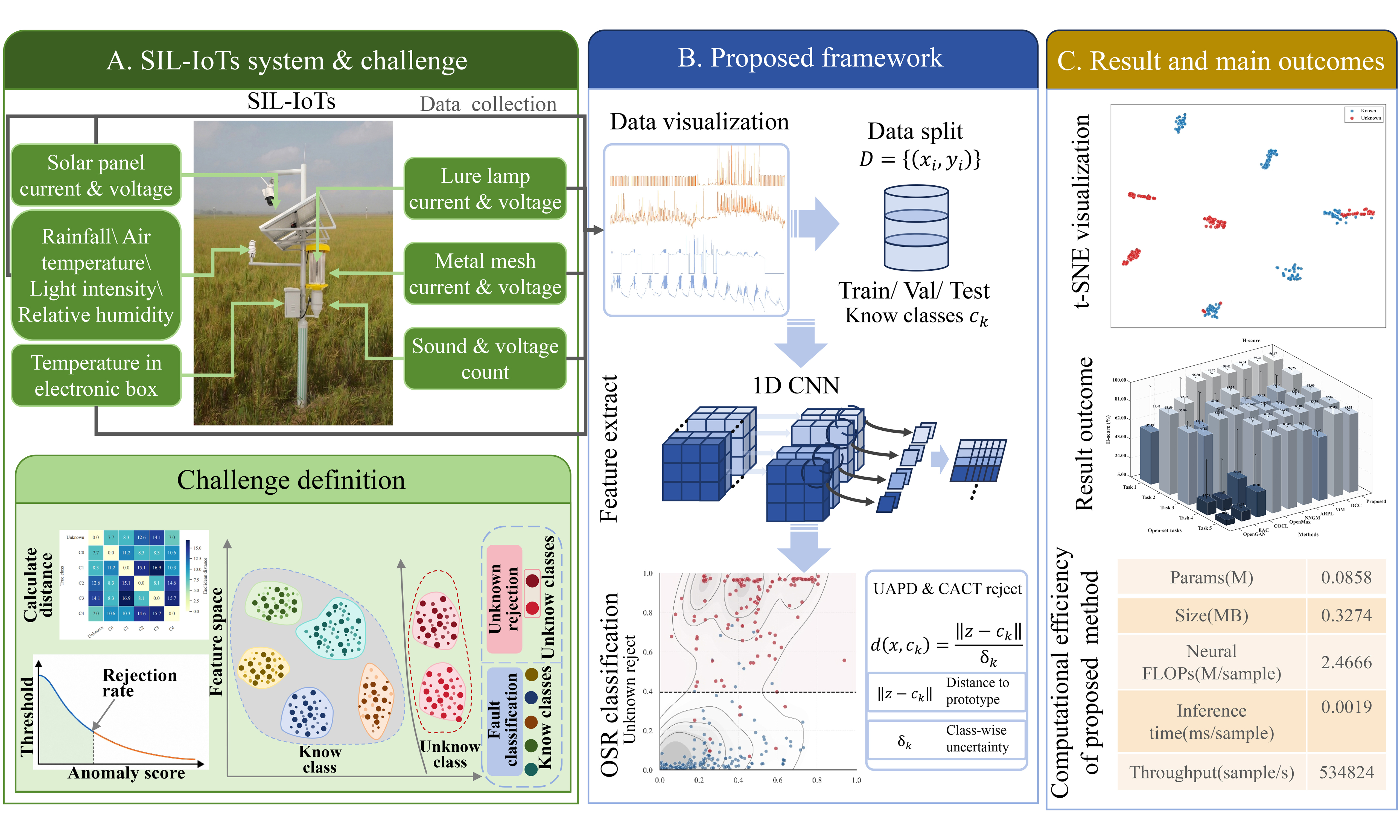
Abstract
Reliable fault diagnosis of field-deployed intelligent agricultural equipment requires not only accurate recognition of known faults but also reliable rejection of previously unseen fault conditions encountered after deployment. This challenge is particularly pronounced in solar insecticidal lamp Internet of Things (SIL-IoTs) systems, where environmental variability, component aging, and operational disturbances can induce substantial intra-class variability and compromise the reliability of conventional closed-set diagnosis. To address this challenge, this article proposes a prototype-based open-set fault diagnosis framework for SIL-IoTs systems. A temporal encoder is trained to extract discriminative representations from multichannel electrical signals. Within the learned feature space, class prototypes are constructed for known faults, and an uncertainty-aware prototype distance (UAPD) is introduced to account for class-wise feature variance during prototype matching. A class-adaptive conformal thresholding (CACT) strategy is further developed to estimate an independent acceptance threshold for each known class using only calibration samples from known classes, thereby enabling open-set rejection without requiring real unknown faults for threshold tuning. Experiments on five open-set diagnosis tasks show that the proposed method achieves the highest overall open-set accuracy across all tasks and the highest H-score in four tasks, with absolute gains of up to 0.0377 over the strongest baseline. These results demonstrate that the proposed framework provides an effective and practically applicable solution for open-set fault diagnosis in field-deployed SIL-IoTs systems.
Keywords


 Download PDF
1. INTRODUCTION
Intelligent systems and machine learning play an important role in modern precision agriculture, where autonomous monitoring, intelligent agricultural equipment, and data-driven maintenance are essential for ensuring reliable long-term field operation[1]. Accordingly, smart agricultural electronic systems are expected to operate autonomously and reliably over extended periods in open-field environments[2]. Recent machine-learning-based studies further demonstrate the capability of data-driven models to capture discriminative temporal features from complex and highly variable data, providing an effective basis for condition monitoring, state assessment, and fault diagnosis in intelligent agricultural systems[3]. Within this context, solar insecticidal lamp Internet of Things (SIL-IoTs) systems represent a typical class of field-deployed intelligent terminals, as they integrate sensing, power supply, communication, and electrical actuation within a continuously operating monitoring platform[4]. By continuously recording multichannel electrical signals during routine operation, these systems facilitate pest monitoring, equipment management, and data-driven agricultural decision-making. In such environments, reliable fault diagnosis is not merely a maintenance requirement but also a prerequisite for trustworthy intelligent sensing and sustained autonomous operation[5].
Most existing intelligent fault diagnosis methods achieve strong performance under closed-set assumptions by using convolutional, recurrent, or hybrid deep networks to learn discriminative representations from time-series data[6]. Related studies in intelligent agriculture have also demonstrated that neural-network- and Gaussian-process-based models can effectively capture nonlinear temporal dependencies and informative dynamic patterns from complex time-series data, providing useful representations for system condition monitoring and fault-related state assessment[7,8]. Although these methods are effective when the training and test label spaces are fully matched, they remain insufficient for realistic open-set deployment[9]. First, a closed-set classifier tends to force an unseen fault into the nearest known category, which may conceal novel failures and mislead maintenance decisions[10]. To alleviate this problem, representative open-set recognition methods have introduced different rejection mechanisms. OpenMax estimates unknown probabilities by modeling the tail distribution of known-class activation distances, ARPL learns reciprocal points to reduce open-space risk, OpenGAN uses adversarially generated samples to regularize the known/unknown boundary, and ViM estimates unknownness from feature residuals and logit information[11-14]. More recent approaches further explore calibrated outlier-class learning, prototype-reciprocal learning, nearest-neighbor Gaussian modeling, and evidential abstention to improve open-set or out-of-distribution decision-making[15-18]. However, these methods are not specifically designed for SIL-IoTs fault diagnosis, where known fault classes may exhibit heterogeneous intra-class dispersion under variable field operating conditions.
Second, even prototype-based or distance-based open-set methods often rely on Euclidean prototype matching, standardized Euclidean distances, Mahalanobis-type post-hoc scoring, or a single global rejection threshold[19,20]. These approaches are closely related to class-conditional distance measures, within-class covariance normalization, and Mahalanobis-type prototype methods, because they normalize distances according to feature scale or covariance information. However, they are usually used as post-hoc statistical decision rules and do not explicitly couple class-wise latent dispersion with known-only class-adaptive threshold calibration. In contrast, the proposed uncertainty-aware prototype distance (UAPD) is embedded in the learned prototype space and uses class-wise latent dispersion to adjust prototype matching for each known fault class. Therefore, UAPD is not introduced as a standalone Mahalanobis classifier, but as a prototype-level uncertainty-aware distance for open-set fault diagnosis. Different known classes may occupy latent regions with very different compactness, and ignoring this can lead to unreliable acceptance boundaries and an unstable trade-off between known-fault recognition and unknown-fault rejection[21].
UAPD also differs from recent prototype-based open-set fault diagnosis methods, which commonly use generated open-set samples, pseudo prototypes, or distance-based rejection rules to model open space[20]. In the proposed framework, unknown-fault samples are not used during training or threshold tuning. Instead, UAPD is combined with class-adaptive conformal thresholding (CACT) to couple class-wise variance-normalized prototype matching with class-specific conformal thresholding estimated from known calibration samples only[22]. This design also differs from auxiliary-set-based generalized zero-shot industrial fault diagnosis, where unseen classes are recognized by transferring auxiliary knowledge, whereas the present open-set setting focuses on rejecting unknown faults without using auxiliary unknown-class data during training or threshold tuning[23].
To address these limitations, this article proposes a prototype-based open-set fault diagnosis framework for SIL-IoTs systems. The framework first learns discriminative temporal representations from multichannel electrical signals by jointly optimizing cross-entropy loss, center loss, and supervised contrastive loss[24]. Based on the learned feature space, one prototype is constructed for each known fault category. Unlike a conventional Mahalanobis-distance classifier, the proposed UAPD performs class-wise variance-normalized prototype matching in the learned latent space. Furthermore, unlike manually tuned or globally shared class-threshold rules, the proposed CACT calibrates one acceptance threshold per known class using conformal nonconformity scores computed only from known calibration samples. In this way, the proposed framework combines discriminative representation learning, adaptive metric design, and class-specific open-set decision-making into a unified diagnosis model.
The main contributions of this article are summarized as follows:
• A prototype-based open-set fault diagnosis framework is proposed for SIL-IoTs systems, unifying known-fault classification and unknown-fault rejection within a single diagnostic framework.
• An UAPD is introduced to account for class-wise feature dispersion, thereby improving the reliability of prototype matching in heterogeneous latent spaces. This design differs from conventional standardized or Mahalanobis-type distance rules by adapting prototype matching to the learned class-wise latent dispersion.
• A CACT strategy is developed to calibrate class-specific rejection boundaries using known-only calibration data. This design improves the balance between known-fault recognition and unknown-fault rejection.
The remainder of this article is organized as follows. Section 2 presents the proposed open-set fault diagnosis framework. Section 3 describes the dataset, task definition, and experimental setup. Section 4 reports the experimental results, including ablation studies and comparisons with competing open-set diagnosis methods. Section 5 discusses the main findings and their implications. Section 6 discusses the limitations of the proposed framework and outlines directions for future improvement. Finally, Section 7 concludes this article.
2. METHODS
2.1. Problem formulation and overview
We consider an open-set diagnosis problem in which each input sample is a multivariate temporal window
where L and F denote the window length and the number of signal channels, respectively. Let the known class set be denoted by
As shown in Figure 1, the proposed framework contains three stages: discriminative representation learning, uncertainty-aware prototype matching, and class-adaptive conformal rejection. First, a temporal encoder maps each signal window to a latent feature vector. Second, one prototype is constructed for each known class from the proper training split, and class-wise feature dispersion is used to define UAPD. Third, the CACT strategy calibrates one rejection threshold per known class by using calibration samples from known classes only. In this way, the final decision rule jointly accounts for class-dependent feature geometry and class-dependent acceptance boundaries.
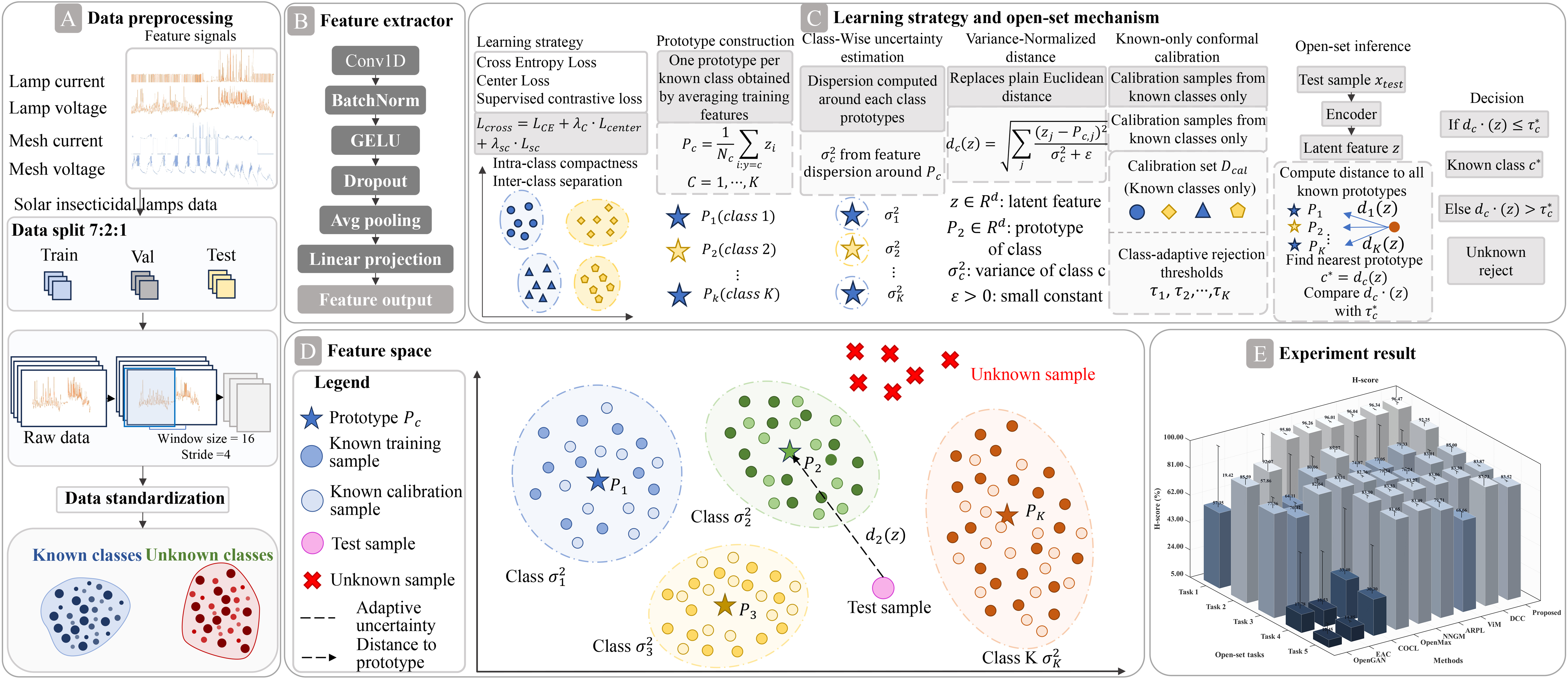
Figure 1. Overview of the proposed open-set diagnosis framework. Raw multichannel electrical signal records are first divided into training, validation, and test subsets, and sliding-window segmentation and standardization are then performed within each subset. A temporal encoder learns latent representations, which are used for prototype construction, uncertainty-aware distance estimation, and class-adaptive open-set rejection. GELU: Gaussian error linear unit.
2.2. Data preprocessing
Following the preprocessing pipeline in Figure 1A, the raw multichannel electrical signal records associated with system operation were first divided into training, validation, and test sets at a ratio of 7:2:1 before window segmentation. The sliding-window operation was then performed separately within each subset, using a window length of 16 and a stride of 4. Therefore, although adjacent windows within the same subset overlap by 75%, no overlapping windows derived from the same acquisition record were shared across the training, validation, and test sets. The generated window samples were standardized before model training, and the normalization parameters were computed using only the training set and then applied unchanged to the validation and test sets. In the implementation, the known-class training data were further divided into a proper training split
For a known training sample (xi, yi) with yi ∈
where fθ(·) denotes the temporal encoder and d is the latent feature dimension. In what follows, we use prototype to refer to the class mean used for open-set inference, and center to refer to the learnable center parameter used only in the training loss. For consistency, class-specific quantities are indexed by the generic class index c ∈
2.3. Temporal encoder and prototype-oriented feature learning
The temporal encoder consists of three stacked 1D convolutional blocks, each followed by batch normalization and Gaussian error linear unit (GELU) activation[27]. Dropout is used for regularization, and adaptive average pooling aggregates the temporal dimension into a fixed-length representation. A linear projection layer then maps the pooled representation to a d-dimensional latent space. In the implementation, d = 64.
To learn a feature space that is both discriminative and compact, we train the encoder jointly with a linear classifier head using three complementary objectives:
where
The center loss is defined as
where
After training, the classifier head is discarded, and the latent space is summarized by one prototype per known class:
where Nc is the number of proper training samples belonging to class c. Unlike the learnable center μc, the prototype Pc is a post-hoc empirical class mean computed from the trained encoder features after representation learning is complete. Thus, Pc reflects the final feature distribution induced by the joint training objective, including the effect of center loss, cross-entropy loss, and supervised contrastive loss. The same post-training features are also used to estimate the class-wise variance vector σc2, so the variance normalization in UAPD is coupled to the learned feature geometry rather than to the learnable center parameters themselves. These prototypes serve as the anchors for the subsequent open-set decision process.
2.4. UAPD
A plain Euclidean distance assumes that all known classes have comparable feature spread in the latent space. This assumption is often too restrictive for open-set diagnosis, because some classes naturally form compact clusters while others remain more dispersed due to operating variability or residual inter-class ambiguity. A uniform metric therefore tends to over-penalize dispersed classes and under-penalize deviations from compact classes[29].
To address this issue, we estimate a class-wise variance vector for each prototype:
Based on Pc and σc2, we define the UAPD between a test feature z and class c as
where ϵ > 0 is a small constant for numerical stability.
This metric can be interpreted as a diagonal Mahalanobis-like prototype distance. Dimensions with low class-wise dispersion contribute more strongly to the distance, whereas naturally noisy dimensions are down-weighted. Consequently, compact classes receive tighter effective boundaries, while broader classes are not unfairly rejected simply because their latent distribution is intrinsically more spread out. The diagonal formulation was adopted as a deliberate design choice to keep the open-set decision rule lightweight, interpretable, and directly aligned with the class-wise uncertainty estimated for each latent feature dimension. A full-covariance Mahalanobis distance can additionally model correlations among latent dimensions, but it requires estimating and inverting one covariance matrix for each known class. This may introduce numerical difficulties when the covariance matrix is ill-conditioned or when strong correlations among latent dimensions make the inverse unstable. It also increases the statistical burden because a full covariance matrix contains many more parameters than a diagonal variance vector, which can make the estimated distance sensitive to the empirical feature distribution of each class. Therefore, we used the diagonal variance vector to preserve the main class-dependent scale information while avoiding the additional numerical and statistical complexity of full-covariance estimation.
Unlike a conventional Mahalanobis-distance classifier, UAPD is not used as an independent post-hoc statistical classifier. Instead, it is embedded in the learned prototype space and uses class-wise latent feature dispersion estimated from the trained encoder features to normalize prototype matching. In this sense, UAPD serves as a class-adaptive prototype-matching metric for open-set diagnosis, rather than as a standalone covariance-based classifier.
2.5. CACT
Although UAPD provides a more faithful distance measure, open-set diagnosis still requires a rejection rule to determine whether the nearest known prototype is sufficiently reliable. A single global threshold is often inadequate because different classes may exhibit markedly different latent-space geometry even after feature learning. We introduce CACT, which calibrates one rejection threshold for each known class by using calibration samples from known classes only[30]. Unlike ordinary class-wise thresholding, the thresholds in CACT are obtained from conformal nonconformity scores rather than manually tuned using unknown samples or an auxiliary unknown set. This design is consistent with the target deployment condition, where real unknown faults are not available during threshold calibration.
The validity of the CACT thresholds relies on the exchangeability assumption of conformal prediction. Specifically, the calibration samples and future deployment samples from the same known class are expected to be generated from the same underlying distribution, or at least to remain approximately exchangeable after preprocessing and feature extraction. Under this condition, the class-specific conformal quantile provides a controlled known-class rejection risk at the prescribed significance level. If substantial distribution shifts occur, such as seasonal variation, sensor drift, component aging, or abrupt changes in operating conditions, the exchangeability assumption may be weakened and the calibrated thresholds may require online updating or recalibration.
For each calibration sample zical from class c, we compute its class-consistent nonconformity score
The threshold for class c is then defined as the upper conformal quantile of the corresponding calibration scores:
where α denotes the target risk level. In our implementation, α = 0.05.
Given a test feature z, we first identify its nearest prototype
The final open-set decision is then made by comparing the nearest-prototype distance with the threshold of the predicted class:
This design avoids tuning on real unknown samples and aligns the acceptance region with class-dependent feature geometry.
2.6. Training and inference procedures
The complete training and inference procedures are summarized in Algorithm 1 and Algorithm 2. Training consists of two stages: discriminative representation learning on the proper known-class training split, followed by prototype, variance, and threshold estimation. Inference uses only the trained encoder, class prototypes, class-wise variances, and class-adaptive thresholds.
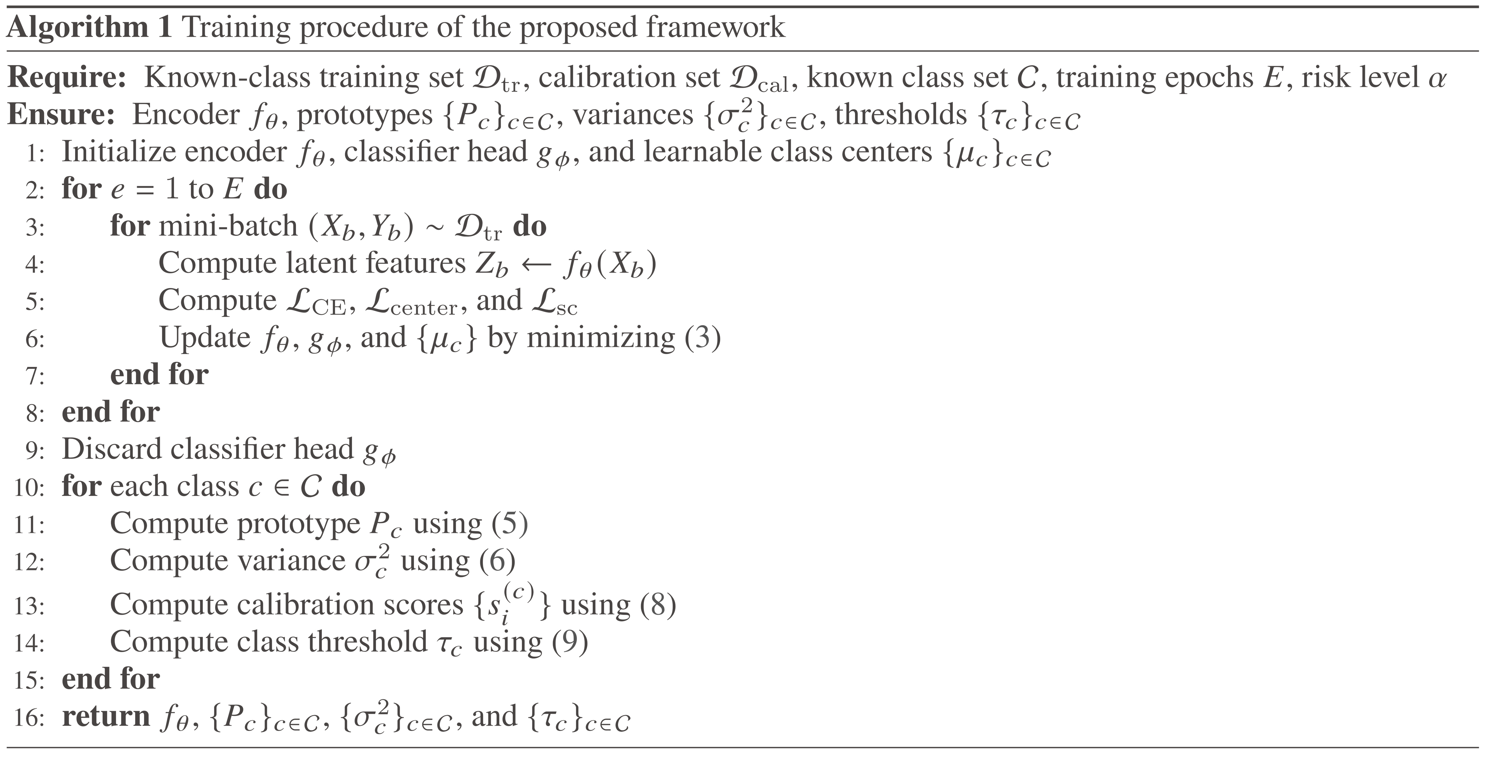
Algorithm 1.
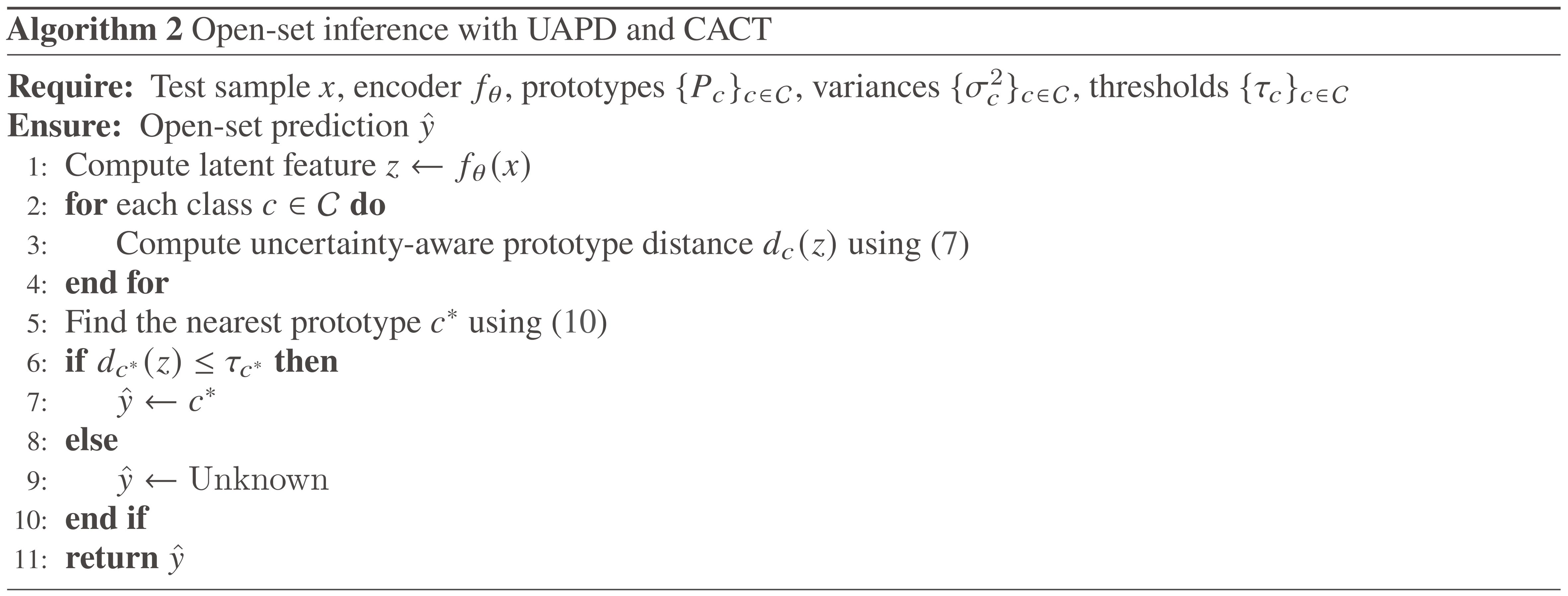
Algorithm 2.
3. DATASET DESCRIPTION AND EXPERIMENTAL SETUP
3.1. Dataset description
The experiments were conducted on real-world multichannel monitoring signals collected from SIL-IoTs systems. As shown in Figure 2, the data used in this study were collected from three field-deployed SIL-IoTs devices in Chuzhou, Anhui Province, China, over a two-month operating period. Following the acquisition protocol of the solar insecticidal lamp fault (SILF) dataset, a raw acquisition record refers to the monitoring segment retained during one fault-diagnosis execution of an SIL-IoTs node. The sensor readings were collected at approximately 0.2 Hz, and each raw acquisition record covered 5 min of device operation. The fault taxonomy is summarized in Table 1, where the fault-free state and eight fault types are denoted by C0-C8.
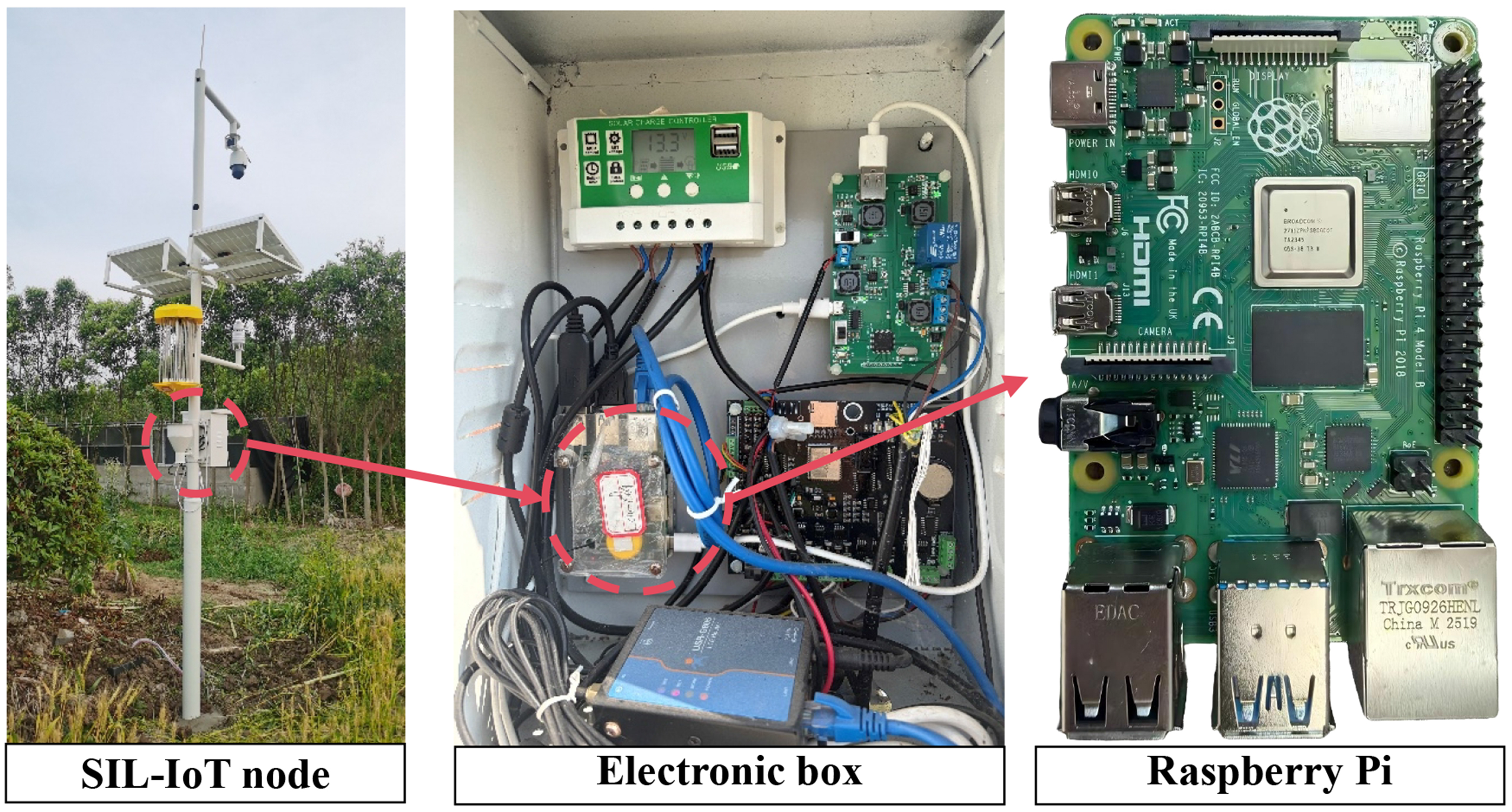
Figure 2. Real-world SIL-IoTs device used for field data collection in Chuzhou, Anhui Province, China. The SIL-IoT node, electronic box, and Raspberry Pi photographs show the actual deployed device, electrical enclosure, and embedded computing unit, respectively, and were taken by the authors. SIL-IoTs: Solar insecticidal lamp Internet of Things.
Taxonomy of fault types and their corresponding class identifiers in SIL-IoTs
| Fault name | Identifier |
| Fault-free | C0 |
| Lure lamp OC | C1 |
| Metal mesh OC | C2 |
| Solar panel OC | C3 |
| Mismatch between light-intensity value and solar panel current value | C4 |
| Metal mesh current value abnormal | C5 |
| Metal mesh voltage value abnormal | C6 |
| Lure lamp current value abnormal | C7 |
| Lure lamp voltage value abnormal | C8 |
Each sample was represented as a temporal window of length 16 with an input dimension of 13. The 13 input features, denoted as Feature 0 to Feature 12, describe the environmental, electrical, and operating states of SIL-IoTs systems, as summarized in Table 2.
Input features used in the experiments
| Description | Feature |
| Ambient air temperature | Feature 0 |
| Ambient relative humidity | Feature 1 |
| Temperature inside the electronic control box | Feature 2 |
| Voltage of the metal mesh | Feature 3 |
| Current of the metal mesh | Feature 4 |
| Voltage of the lure lamp | Feature 5 |
| Current of the lure lamp | Feature 6 |
| Voltage of the solar panel | Feature 7 |
| Current of the solar panel | Feature 8 |
| Measured light intensity | Feature 9 |
| Voltage-related count feature | Feature 10 |
| Sound-related count feature | Feature 11 |
| Voltage output of the rainfall sensor | Feature 12 |
The raw monitoring records were first divided into training, validation, and test subsets at a ratio of 7:2:1 before sliding-window segmentation. The sliding-window operation was then performed independently within each subset using a window length of 16 and a stride of 4. After preprocessing, 500 window samples were retained for each fault category, resulting in 4,500 window samples. Therefore, no obvious sample imbalance was present across the nine categories. For each known class in an open-set task, 350, 100, and 50 window samples were used for training, validation, and testing, respectively. Unknown-class samples were excluded from training and were used only in the validation and test stages. Because the experimental subset was generated and balanced after sliding-window segmentation, the class-wise experimental scale is reported at the window-sample level.
This partition protocol was used to reduce the risk of temporal leakage caused by overlapping windows. Specifically, the generated windows were not randomly mixed across the training, validation, and test subsets. Normalization parameters were estimated only from the training data and then applied unchanged to the validation and test data. The training and test data were collected from different SIL-IoTs devices and operating conditions, while the acquisition dates were matched to reduce date-related bias.
To evaluate the proposed method under realistic open-set conditions, only known fault classes were used during training. Unknown fault classes were excluded from model fitting and introduced only during validation and testing. As shown in Figure 3, the inter-class distances were highly non-uniform, and several class pairs were substantially closer than others. The class-center distance map in Figure 3A was used only to guide the construction of the five open-set task partitions and was not used for model training, model selection, prototype estimation, or threshold tuning. Based on this distance distribution, five open-set diagnosis tasks were constructed by varying the partition between known and unknown classes, as summarized in Figure 3B and Table 3. Following the revised task order, Task 1 represents a relatively simple open-set setting. Task 2 and Task 3 introduce more ambiguous unknown-class combinations. Task 4 increases the number of unknown classes, while Task 5 is treated as the most challenging setting because its unknown set contains multiple lamp- and metal-mesh-related current or voltage faults that are close to several known classes in the distance map.
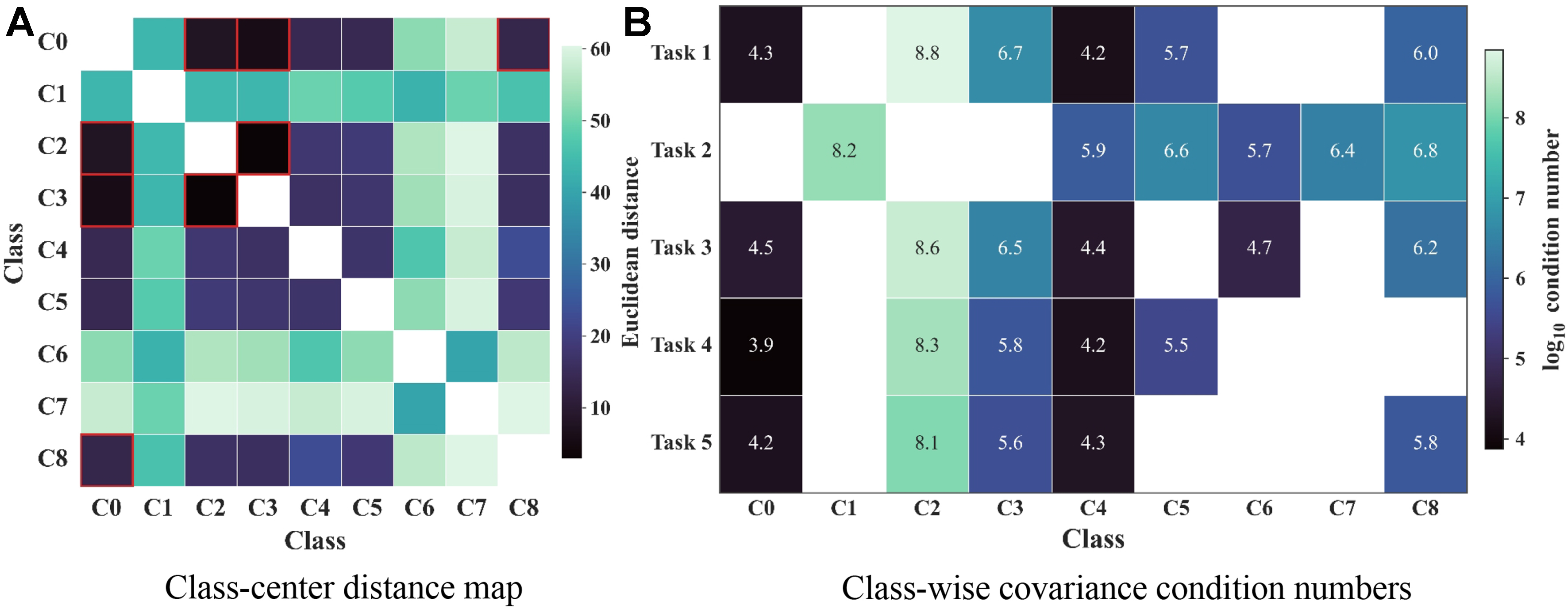
Figure 3. Class-center distance and covariance condition analysis. (A) Normalized class-center Euclidean distance map used to guide open-set task construction. Darker cells indicate smaller inter-class distances, and red boxes highlight closely spaced class pairs; (B) Class-wise full-covariance condition numbers estimated from latent features in the proper training split. Larger values indicate greater potential numerical instability when applying full-covariance Mahalanobis distance.
Definition of the five open-set diagnosis tasks
| Task | Known classes | Unknown classes |
| Task 1 | C0 C2 C3 C4 C5 C8 | C1 C6 C7 |
| Task 2 | C1 C4 C5 C6 C7 C8 | C0 C2 C3 |
| Task 3 | C0 C2 C3 C4 C6 C8 | C1 C5 C7 |
| Task 4 | C0 C2 C3 C4 C5 | C1 C6 C7 C8 |
| Task 5 | C0 C2 C3 C4 C8 | C1 C5 C6 C7 |
In the implemented pipeline, the known-class training set was further divided into a proper training split and a calibration split. The proper training split was used for representation learning, prototype estimation, and class-wise variance estimation. The calibration split was used only for class-adaptive threshold estimation. No samples from the unknown classes were used for model fitting, prototype construction, variance estimation, threshold calibration, or hyperparameter selection. The same training, validation, and test protocol was applied to all compared methods in every task to ensure a fair comparison. This setup is consistent with the intended deployment setting, in which unknown samples are unavailable during threshold tuning.
3.2. Experimental setup
3.2.1. Implementation details
The proposed framework is implemented using the prototype-based architecture described in Section 2. Specifically, the temporal encoder consists of three stacked 1D convolutional layers with channel dimensions of 64, 128, and 128, respectively. Each convolutional layer is followed by batch normalization and GELU activation, and dropout with a rate of 0.15 is used for regularization. Adaptive average pooling is then applied to aggregate temporal information, and a linear projection layer maps the pooled representation into a 64-dimensional latent space.
During training, the encoder is jointly optimized with a linear classifier head over the known classes. The training objective combines cross-entropy loss, center loss, and supervised contrastive loss, with weights of 0.03 and 0.10 assigned to the center-loss and supervised-contrastive terms, respectively. The model is trained for 80 epochs using AdamW with a batch size of 64, a learning rate of 10-3, and a weight decay of 10-4. A cosine annealing learning-rate scheduler is employed throughout training.
For open-set inference, one prototype is constructed for each known class by averaging the latent features of the proper training samples. The class-wise feature variance is then estimated from the same split and used to define the UAPD. The calibration subset occupies 20% of the known training data and is used only to estimate class-adaptive conformal thresholds with a risk level of α = 0.05. It is not used for representation learning, prototype estimation, hyperparameter selection, or model selection.
All experiments are implemented in Python 3.11 and PyTorch 2.7.1 with CUDA 12.8 on an NVIDIA RTX 5070 GPU. Each experiment is repeated with five different random seeds (42, 123, 2024, 3407, 2026), and all reported results are presented as mean ± standard deviation.
3.2.2. Evaluation metrics
To evaluate open-set diagnosis performance, four primary metrics are adopted, namely OS, OS′, UNK, and H-score[31]. Specifically, OS denotes the overall classification accuracy over all test samples, OS′ denotes the classification accuracy over known-class samples only, and UNK represents the detection rate of unknown fault samples:
where C and N denote the numbers of correctly classified and total test samples, respectively; CK and NK denote the numbers of correctly classified and total known-class samples; and CU and NU denote the numbers of correctly rejected and total unknown samples.
The H-score is defined as the harmonic mean of OS′ and UNK:
A higher H-score indicates a better balance between known-fault recognition and unknown-fault rejection.
3.2.3. Comparative methods
To assess the effectiveness of the proposed framework, we compare it against representative open-set recognition and open-set fault diagnosis methods under the same task definitions, preprocessing pipeline, data partitions, and evaluation protocol. For a fair comparison, all comparative methods are implemented with the same 1D convolutional encoder, which consists of three one-dimensional convolutional blocks followed by adaptive average pooling and a linear projection layer. Therefore, the performance differences among these comparative methods mainly reflect their open-set scoring and rejection mechanisms rather than differences in the feature-extraction backbone.
• OpenMax[11]: a classical open-set recognition baseline that models the tail distribution of known-class activation distances and adjusts prediction scores to estimate unknown probabilities.
• ARPL[12]: an adversarial reciprocal-point learning method that enhances open-set separation by jointly learning discriminative features and class-reciprocal representations.
• OpenGAN[13]: an open-set adversarial learning framework that uses generative adversarial training to distinguish known samples from potential unknown samples.
• ViM[14]: a post hoc open-set recognition method that combines feature-space residual information and logit structure to estimate unknownness.
• COCL[15]: a calibrated outlier-class learning method that introduces an auxiliary outlier class to improve the separation between known and outlier samples.
• DCC[16]: a recent prototype-learning-based open-set fault diagnosis method that jointly uses prototypical points and reciprocal points to reduce empirical classification risk and open-space risk.
• NNGM[17]: a nearest-neighbor Gaussian modeling baseline that combines local neighborhood distance and class-conditional Gaussian feature modeling to estimate the unknownness score in the learned feature space.
• EAC[18]: an evidential abstention classifier that quantifies prediction uncertainty and rejects samples with insufficient evidence for known-class assignment.
For all comparative methods, the rejection thresholds are determined using only the known-class calibration set, without using real unknown samples. The main hyperparameters, including the learning rate, batch size, number of training epochs, latent dimension, calibration ratio, and significance level, are kept consistent across methods unless a method-specific parameter is required. Method-specific hyperparameters are set according to the corresponding original methods or kept at the default settings recommended in their implementations. The implementation details of the comparative methods are summarized in Table 4.
Implementation details of the comparative methods, including backbone, rejection score, threshold data, and main hyperparameters
| Method | Backbone | Rejection score/threshold | Threshold data | Main hyperparameters |
| OpenGAN | 1D-CNN encoder | Unknown/outlier logit score Conformal quantile threshold | Known-class only | Latent dimension = 64 Learning rate = 10-3 Weight decay = 10-4 α = 0.05 |
| EAC | 1D-CNN encoder | Evidential uncertainty score Conformal quantile threshold | Known-class only | Evidence L1 weight = 0.001 Pseudo-evidence weight = 0.05 KL annealing epochs = 10 |
| COCL | 1D-CNN encoder | Calibrated outlier-class score Conformal quantile threshold | Known-class only | Outlier weight = 0.40 Known margin = 1.0 Margin weight = 0.10 |
| OpenMax | 1D-CNN encoder | Weibull-calibrated OpenMax score Conformal quantile threshold | Known-class only | Tail size = 20 Alpha rank = 3 α = 0.05 Calibration = 20% Latent dimension = 64 |
| NNGM | 1D-CNN encoder | Nearest-neighbor score Gaussian feature-space score Conformal quantile threshold | Known-class only | Latent dimension = 64 Supervised contrastive weight = 0.10 α = 0.05 |
| ARPL | 1D-CNN encoder | Reciprocal-point distance score Conformal quantile threshold | Known-class only | Reciprocal margin = 4.0 Compact weight = 0.01 Reciprocal weight = 0.10 α = 0.05 |
| ViM | 1D-CNN encoder | Virtual-logit score Feature-residual score Conformal quantile threshold | Known-class only | Explained variance ratio = 0.95 α = 0.05 Calibration = 20% |
| DCC | 1D-CNN encoder | Prototype distance score Reciprocal-point distance score Conformal quantile threshold | Known-class only | Prototype weight = 0.01 Reciprocal weight = 0.10 Prototype margin = 2.0 Reciprocal margin = 4.0 |
| Proposed | 1D-CNN encoder | UAPD-based open-set score Known-only conformal threshold | Known-class only | α = 0.05 Calibration = 20% Latent dimension = 64 Dropout = 0.15 |
4. RESULTS
4.1. Ablation experiment
As summarized in Table 5, a key question is whether the gain of the full model arises from the combined action of UAPD and CACT, rather than from a single dominant component. Across the five tasks, the complete model achieved the highest OS in Task 1 to Task 4, reaching 0.9689, 0.9333, 0.8849, and 0.8618, respectively, and obtained an OS of 0.8524 in Task 5. These results indicate that enabling both modules generally improves overall open-set performance, although the advantage is not uniform across all task settings. The full model also produced the highest H-score in Task 1 and Task 2, and remained competitive in Task 3 to Task 5, supporting the view that the joint design improves the overall balance between known-class recognition and unknown-class rejection. A more detailed comparison suggests that the two modules play distinct roles. Removing UAPD caused the most pronounced degradation in Task 2, where OS, UNK, and H-score dropped from 0.9333, 0.8960, and 0.9225 to 0.8493, 0.6013, and 0.7435, despite an increase in OS′ to 0.9733. This pattern is consistent with a shift towards known-class bias at the expense of open-set robustness. By contrast, removing CACT led to higher UNK and H-score in Task 3 and Task 5, and also produced a higher OS in Task 5, indicating that CACT mainly adjusts the trade-off between known-class recognition and unknown-class rejection rather than uniformly maximizing every metric in every task. Notably, UNK was saturated in Task 1 and Task 4 across all variants, which limits mechanistic interpretation in these relatively easy settings. Together, these ablations show that the full configuration provides a strong and balanced operating point overall, while also indicating that the effect of CACT on unknown-class discrimination remains task-dependent.
Ablation study across five tasks
| Task | Method | UAPD | CACT | OS | OS′ | UNK | H-score |
| Task 1 | Baseline | 0.9573 ± 0.0043 | 0.9360 ± 0.0064 | 1.0000 ± 0.0000 | 0.9669 ± 0.0034 | ||
| w/o UAPD | √ | 0.9609 ± 0.0060 | 0.9413 ± 0.0090 | 1.0000 ± 0.0000 | 0.9698 ± 0.0048 | ||
| w/o CACT | √ | 0.9542 ± 0.0051 | 0.9313 ± 0.0077 | 1.0000 ± 0.0000 | 0.9644 ± 0.0041 | ||
| Proposed | √ | √ | 0.9689 ± 0.0082 | 0.9533 ± 0.0122 | 1.0000 ± 0.0000 | 0.9761 ± 0.0065 | |
| Task 2 | Baseline | 0.9293 ± 0.0091 | 0.9533 ± 0.0211 | 0.8813 ± 0.0498 | 0.9149 ± 0.0197 | ||
| w/o UAPD | √ | 0.8493 ± 0.0826 | 0.9733 ± 0.0041 | 0.6013 ± 0.2487 | 0.7435 ± 0.2389 | ||
| w/o CACT | √ | 0.9320 ± 0.0090 | 0.9580 ± 0.0132 | 0.8800 ± 0.0490 | 0.9165 ± 0.0211 | ||
| Proposed | √ | √ | 0.9333 ± 0.0093 | 0.9520 ± 0.0198 | 0.8960 ± 0.0361 | 0.9225 ± 0.0142 | |
| Task 3 | Baseline | 0.8507 ± 0.0234 | 0.9493 ± 0.0060 | 0.6533 ± 0.0682 | 0.7724 ± 0.0464 | ||
| w/o UAPD | √ | 0.8369 ± 0.0213 | 0.9360 ± 0.0138 | 0.6387 ± 0.0635 | 0.7576 ± 0.0461 | ||
| w/o CACT | √ | 0.8836 ± 0.0297 | 0.9027 ± 0.0119 | 0.8453 ± 0.0874 | 0.8711 ± 0.0469 | ||
| Proposed | √ | √ | 0.8849 ± 0.0079 | 0.9387 ± 0.0084 | 0.7773 ± 0.0342 | 0.8500 ± 0.0175 | |
| Task 4 | Baseline | 0.8600 ± 0.0061 | 0.9480 ± 0.0110 | 0.7500 ± 0.0000 | 0.8374 ± 0.0043 | ||
| w/o UAPD | √ | 0.8600 ± 0.0042 | 0.9480 ± 0.0075 | 0.7500 ± 0.0000 | 0.8374 ± 0.0029 | ||
| w/o CACT | √ | 0.8596 ± 0.0058 | 0.9472 ± 0.0104 | 0.7500 ± 0.0000 | 0.8371 ± 0.0040 | ||
| Proposed | √ | √ | 0.8618 ± 0.0064 | 0.9512 ± 0.0115 | 0.7500 ± 0.0000 | 0.8387 ± 0.0045 | |
| Task 5 | Baseline | 0.8404 ± 0.0062 | 0.8992 ± 0.0158 | 0.7670 ± 0.0152 | 0.8277 ± 0.0062 | ||
| w/o UAPD | √ | 0.8413 ± 0.0051 | 0.9120 ± 0.0063 | 0.7530 ± 0.0045 | 0.8249 ± 0.0049 | ||
| w/o CACT | √ | 0.8627 ± 0.0197 | 0.9264 ± 0.0067 | 0.7830 ± 0.0373 | 0.8484 ± 0.0240 | ||
| Proposed | √ | √ | 0.8524 ± 0.0026 | 0.9344 ± 0.0046 | 0.7500 ± 0.0000 | 0.8321 ± 0.0018 |
4.2. Hyperparameter sensitivity analysis
To examine the robustness of the selected hyperparameters, we further conducted sensitivity analysis for the main parameters of the proposed framework, including the CACT significance level α, the calibration split, the center-loss weight λc, the supervised-contrastive-loss weight λsc, and the numerical stabilizer ϵ in UAPD. The dropout rate was kept at 0.15 as an encoder regularization setting, while the sensitivity analysis focuses on the parameters that directly affect prototype compactness, variance normalization, and conformal rejection. The results are summarized in Table 6, where the default settings used in the proposed method are highlighted in bold.
Sensitivity analysis of the main hyperparameters across five open-set diagnosis tasks
| Parameter | Value | Task 1 | Task 2 | Task 3 | Task 4 | Task 5 | |||||
| OS | H-score | OS | H-score | OS | H-score | OS | H-score | OS | H-score | ||
| α | 0.01 | 0.8964 ± 0.1474 | 0.7766 ± 0.4342 | 0.7347 ± 0.0905 | 0.3082 ± 0.3235 | 0.7693 ± 0.0890 | 0.6083 ± 0.2975 | 0.7640 ± 0.1507 | 0.6531 ± 0.3652 | 0.8253 ± 0.0092 | 0.8121 ± 0.0070 |
| 0.03 | 0.9378 ± 0.0141 | 0.9372 ± 0.0113 | 0.7347 ± 0.0905 | 0.3082 ± 0.3235 | 0.7693 ± 0.0890 | 0.6083 ± 0.2975 | 0.7640 ± 0.1507 | 0.6531 ± 0.3652 | 0.8253 ± 0.0092 | 0.8121 ± 0.0070 | |
| 0.05 | 0.9689 ± 0.0082 | 0.9761 ± 0.0065 | 0.9333 ± 0.0093 | 0.9225 ± 0.0142 | 0.8849 ± 0.0079 | 0.8500 ± 0.0175 | 0.8618 ± 0.0064 | 0.8387 ± 0.0045 | 0.8524 ± 0.0026 | 0.8321 ± 0.0018 | |
| 0.10 | 0.9227 ± 0.0079 | 0.9384 ± 0.0067 | 0.8898 ± 0.0316 | 0.8554 ± 0.0623 | 0.8382 ± 0.0091 | 0.8076 ± 0.0225 | 0.8111 ± 0.0152 | 0.8011 ± 0.0117 | 0.8191 ± 0.0177 | 0.8107 ± 0.0197 | |
| Calibration | 10% | 0.9338 ± 0.0062 | 0.9477 ± 0.0051 | 0.7271 ± 0.0645 | 0.3101 ± 0.2810 | 0.8373 ± 0.0312 | 0.7911 ± 0.0467 | 0.7760 ± 0.1570 | 0.6620 ± 0.3701 | 0.8187 ± 0.0060 | 0.8097 ± 0.0092 |
| 15% | 0.9387 ± 0.0088 | 0.9517 ± 0.0072 | 0.7244 ± 0.0641 | 0.2917 ± 0.2835 | 0.7924 ± 0.0406 | 0.7176 ± 0.1116 | 0.7680 ± 0.1558 | 0.6561 ± 0.3673 | 0.8280 ± 0.0066 | 0.8142 ± 0.0049 | |
| 20% | 0.9689 ± 0.0082 | 0.9761 ± 0.0065 | 0.9333 ± 0.0093 | 0.9225 ± 0.0142 | 0.8849 ± 0.0079 | 0.8500 ± 0.0175 | 0.8618 ± 0.0064 | 0.8387 ± 0.0045 | 0.8524 ± 0.0026 | 0.8321 ± 0.0018 | |
| 30% | 0.9271 ± 0.0082 | 0.9421 ± 0.0069 | 0.8391 ± 0.0388 | 0.7134 ± 0.0904 | 0.8236 ± 0.0174 | 0.7698 ± 0.0171 | 0.8422 ± 0.0057 | 0.8247 ± 0.0041 | 0.8133 ± 0.0063 | 0.8029 ± 0.0049 | |
| λc | 0 | 0.7831 ± 0.1785 | 0.5583 ± 0.5097 | 0.7462 ± 0.0546 | 0.4160 ± 0.2110 | 0.8116 ± 0.0150 | 0.7523 ± 0.0196 | 0.6489 ± 0.1797 | 0.3308 ± 0.4530 | 0.8098 ± 0.0119 | 0.8001 ± 0.0093 |
| 0.01 | 0.9204 ± 0.0250 | 0.9362 ± 0.0215 | 0.7516 ± 0.0825 | 0.4134 ± 0.2735 | 0.8098 ± 0.0422 | 0.7182 ± 0.1126 | 0.7089 ± 0.1848 | 0.4955 ± 0.4523 | 0.8147 ± 0.0095 | 0.8039 ± 0.0074 | |
| 0.03 | 0.9689 ± 0.0082 | 0.9761 ± 0.0065 | 0.9333 ± 0.0093 | 0.9225 ± 0.0142 | 0.8849 ± 0.0079 | 0.8500 ± 0.0175 | 0.8618 ± 0.0064 | 0.8387 ± 0.0045 | 0.8524 ± 0.0026 | 0.8321 ± 0.0018 | |
| 0.10 | 0.9373 ± 0.0062 | 0.9507 ± 0.0051 | 0.7338 ± 0.0694 | 0.3444 ± 0.2790 | 0.8240 ± 0.0123 | 0.7622 ± 0.0109 | 0.8320 ± 0.0185 | 0.8170 ± 0.0141 | 0.8280 ± 0.0128 | 0.8169 ± 0.0154 | |
| λsc | 0 | 0.9231 ± 0.0314 | 0.9383 ± 0.0272 | 0.7524 ± 0.0876 | 0.4053 ± 0.2977 | 0.7889 ± 0.0331 | 0.6890 ± 0.0921 | 0.7760 ± 0.1428 | 0.6580 ± 0.3680 | 0.8164 ± 0.0085 | 0.8062 ± 0.0064 |
| 0.05 | 0.9364 ± 0.0110 | 0.9499 ± 0.0090 | 0.7502 ± 0.0846 | 0.3941 ± 0.3018 | 0.8120 ± 0.0145 | 0.7477 ± 0.0159 | 0.7684 ± 0.1522 | 0.6560 ± 0.3669 | 0.8196 ± 0.0091 | 0.8077 ± 0.0070 | |
| 0.10 | 0.9689 ± 0.0082 | 0.9761 ± 0.0065 | 0.9333 ± 0.0093 | 0.9225 ± 0.0142 | 0.8849 ± 0.0079 | 0.8500 ± 0.0175 | 0.8618 ± 0.0064 | 0.8387 ± 0.0045 | 0.8524 ± 0.0026 | 0.8321 ± 0.0018 | |
| 0.20 | 0.9280 ± 0.0098 | 0.9429 ± 0.0081 | 0.7591 ± 0.0784 | 0.4372 ± 0.2753 | 0.8209 ± 0.0087 | 0.7613 ± 0.0033 | 0.7667 ± 0.1529 | 0.6549 ± 0.3664 | 0.8209 ± 0.0075 | 0.8106 ± 0.0084 | |
| ϵ | 10-8 | 0.9382 ± 0.0040 | 0.9514 ± 0.0033 | 0.7520 ± 0.0859 | 0.4013 ± 0.3028 | 0.8129 ± 0.0119 | 0.7537 ± 0.0110 | 0.7631 ± 0.1501 | 0.6524 ± 0.3649 | 0.8231 ± 0.0091 | 0.8104 ± 0.0069 |
| 10-6 | 0.9689 ± 0.0082 | 0.9761 ± 0.0065 | 0.9333 ± 0.0093 | 0.9225 ± 0.0142 | 0.8849 ± 0.0079 | 0.8500 ± 0.0175 | 0.8618 ± 0.0064 | 0.8387 ± 0.0045 | 0.8524 ± 0.0026 | 0.8321 ± 0.0018 | |
| 10-4 | 0.9467 ± 0.0059 | 0.9583 ± 0.0048 | 0.7596 ± 0.0764 | 0.4416 ± 0.2551 | 0.8151 ± 0.0157 | 0.7465 ± 0.0248 | 0.7653 ± 0.1503 | 0.6537 ± 0.3656 | 0.8302 ± 0.0105 | 0.8158 ± 0.0079 | |
| 10-2 | 0.8222 ± 0.1787 | 0.5756 ± 0.5256 | 0.7849 ± 0.0690 | 0.5353 ± 0.2321 | 0.6973 ± 0.0751 | 0.3646 ± 0.2902 | 0.7022 ± 0.1920 | 0.4948 ± 0.4517 | 0.8356 ± 0.0103 | 0.8198 ± 0.0076 | |
Overall, the sensitivity results show that the selected default settings provide a stable operating point across the five tasks. For α, excessively small values weakened unknown rejection in several tasks, whereas α = 0.05 maintained a better balance between OS and H-score. For the calibration split, the 20% setting generally achieved stronger, more stable performance than the 10% or 15% settings, while the 30% setting reduced the amount of data available for representation and prototype learning. The loss-weight results show that both λc and λsc are useful: setting either weight to zero degraded performance, whereas the default values preserved compact known-class representations and improved open-set balance. The results for ϵ indicate that a small stabilizer is sufficient for UAPD, whereas an overly large value can weaken variance normalization.
4.3. State-of-the-art open-set diagnosis methods compared
As shown in Figure 4, the proposed method achieved the highest OS in Tasks 1-4 and remained competitive in Task 5 when compared with OpenMax, OpenGAN, EAC, COCL, NNGM, ARPL, ViM, and DCC. This result indicates that the proposed framework provides strong overall open-set diagnosis performance by jointly considering known-class recognition and unknown-class rejection. Although several comparative methods achieved competitive results in individual tasks, their performance fluctuated more noticeably across task settings, whereas the proposed method maintained consistently high OS accuracy.
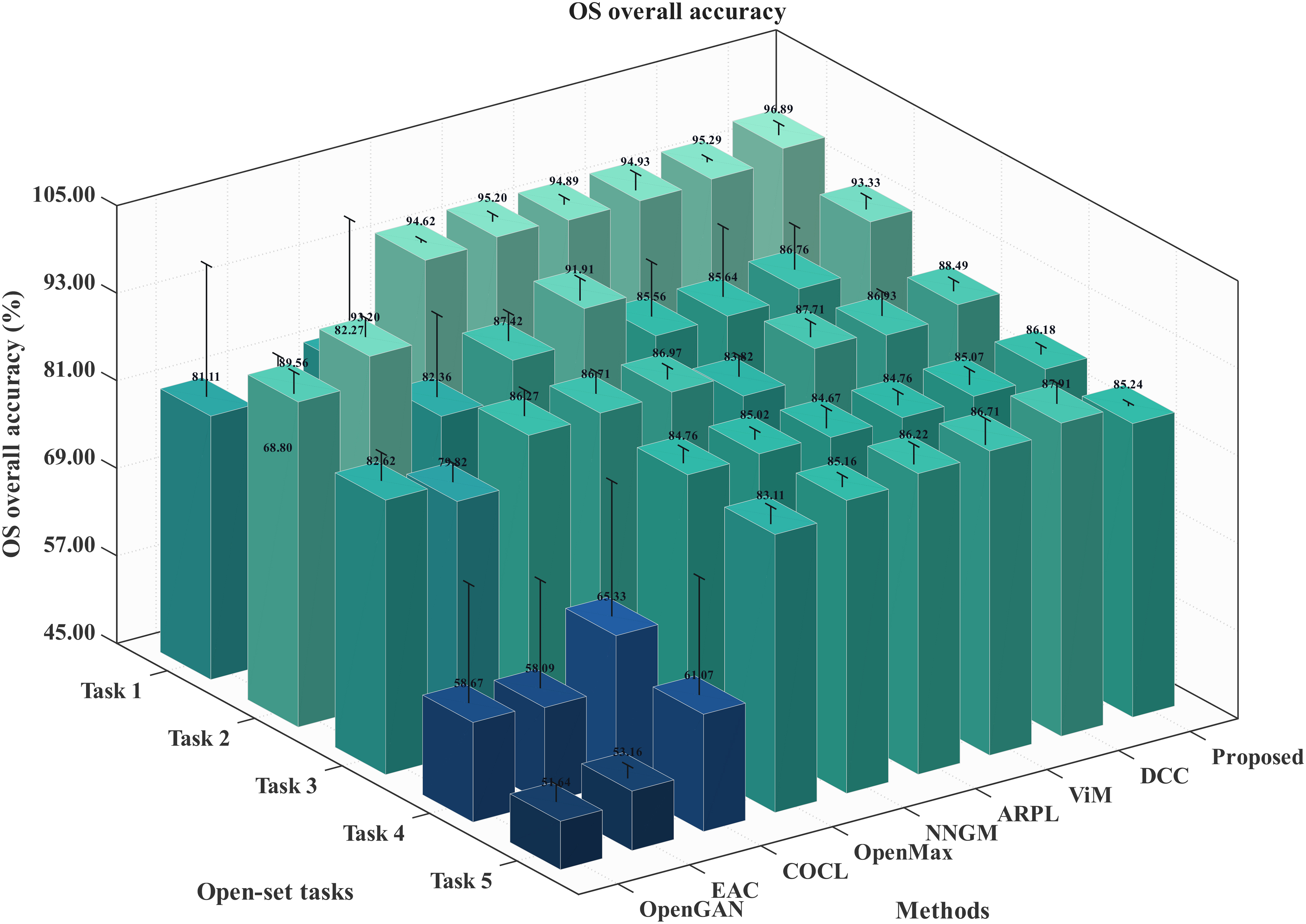
Figure 4. Comparison of OS overall accuracy across five open-set tasks.
As shown in Figure 5, the proposed method also preserved strong known-class recognition performance. The OS′ results indicate that introducing unknown rejection does not substantially weaken the classification of known SIL-IoTs fault categories. Compared with the baseline methods, the proposed framework maintains more stable known-class accuracy across different open-set partitions, suggesting that the learned prototype representation remains discriminative for known faults.
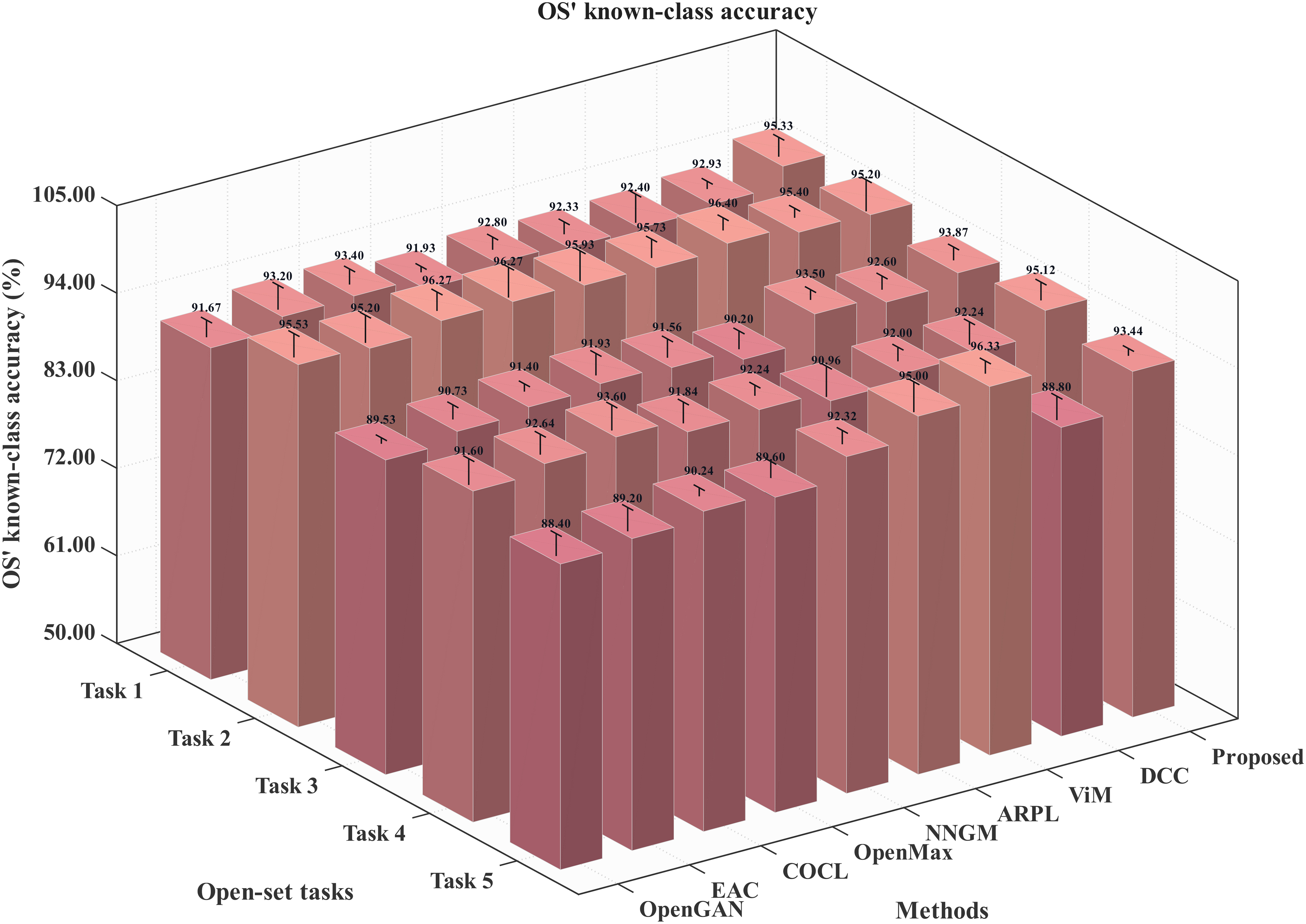
Figure 5. Comparison of OS′ known-class accuracy across five open-set tasks.
As shown in Figure 6, the proposed method achieved the best or highly competitive H-scores across the five tasks. Since H-score jointly measures the balance between known-class recognition and unknown-class detection, these results further confirm that the proposed method achieves more balanced decision behavior than the compared methods. The advantage is especially evident in challenging tasks where unknown samples are close to known fault categories.
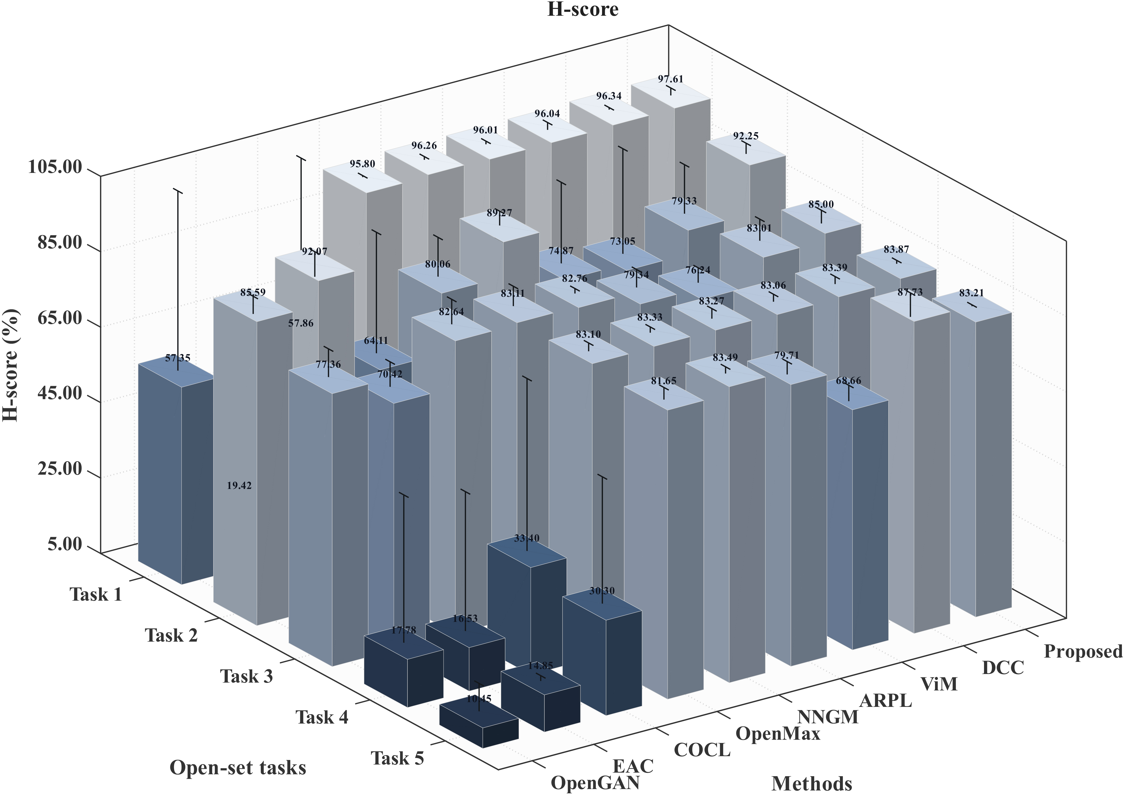
Figure 6. Comparison of H-score across five open-set tasks.
As shown in Figure 7, the proposed method achieved strong UNK performance, demonstrating its ability to reject previously unseen fault types. Compared with OpenMax, OpenGAN, EAC, COCL, NNGM, ARPL, ViM, and DCC, the proposed method more effectively reduced misclassification of unknown samples as known categories. This improvement can be attributed to the UAPD and CACT, which jointly refine prototype matching and unknown rejection.
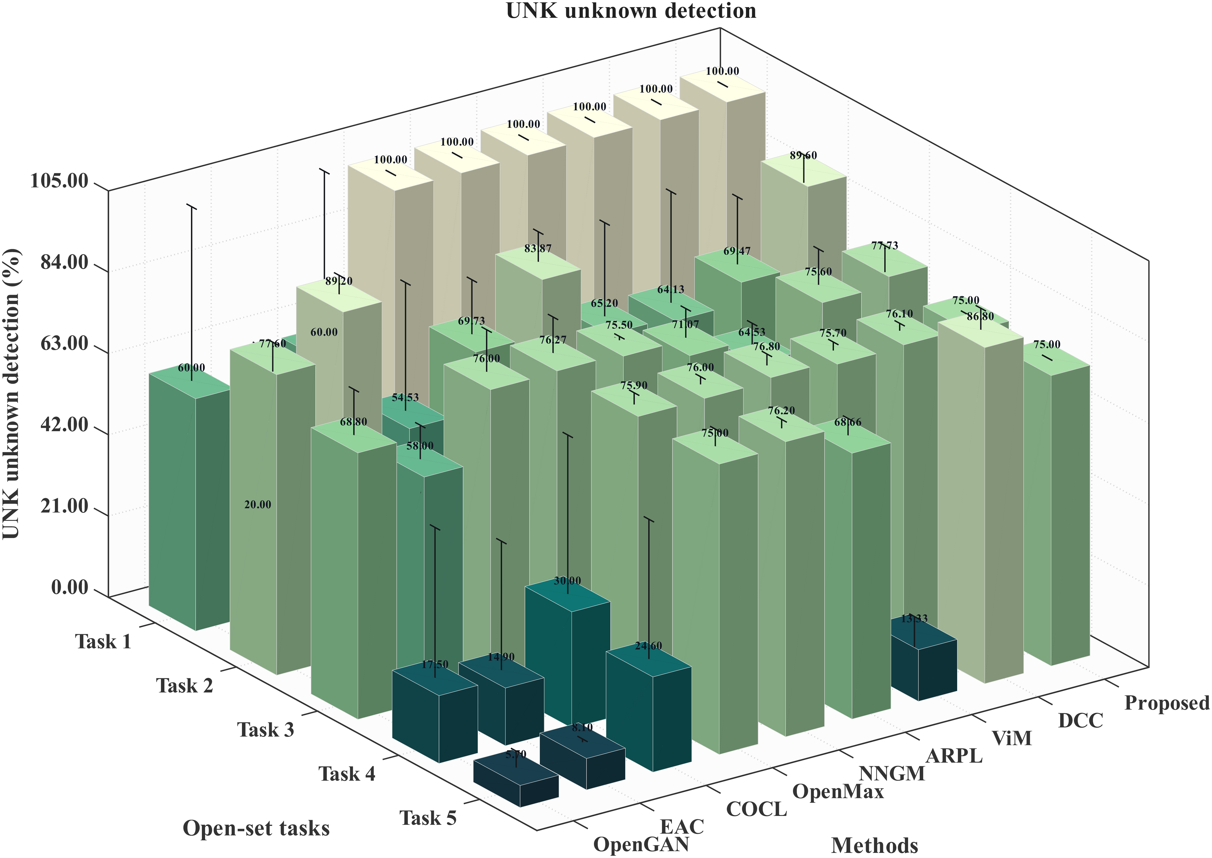
Figure 7. Comparison of UNK unknown-detection accuracy across five open-set tasks.
4.4. Computational efficiency analysis
To evaluate the proposed framework’s suitability for resource-constrained SIL-IoT devices, we further compared the computational cost and inference efficiency of the proposed method with the baseline methods. All methods were evaluated using the same input size, the same 1D convolutional backbone, and the same batch inference setting. The number of parameters, model size, neural forward floating-point operations (FLOPs), additional open-set mechanism FLOPs, inference latency, and throughput are summarized in Table 7.
Computational efficiency comparison of the proposed method and baseline methods
| Method | Params (M) | Size (MB) | Neural FLOPs (M/sample) | OSR FLOPs (K/sample) | Inference time (ms/sample) | Throughput (samples/s) |
| OpenMax | 0.0858 | 0.3274 | 2.4666 | 1.272 | 0.0018 | 546698 |
| OpenGAN | 0.0859 | 0.3277 | 2.4667 | 0.006 | 0.0018 | 559289 |
| EAC | 0.0858 | 0.3274 | 2.4666 | 0.024 | 0.0020 | 498254 |
| COCL | 0.0859 | 0.3277 | 2.4667 | 0.390 | 0.0018 | 545303 |
| NNGM | 0.0858 | 0.3274 | 2.4666 | 323.712 | 0.0018 | 545534 |
| ARPL | 0.0862 | 0.3289 | 2.4658 | 0.768 | 0.0024 | 419252 |
| ViM | 0.0858 | 0.3274 | 2.4666 | 8.576 | 0.0019 | 530625 |
| DCC | 0.0862 | 0.3289 | 2.4658 | 1.536 | 0.0031 | 321537 |
| Proposed | 0.0858 | 0.3274 | 2.4666 | 1.542 | 0.0019 | 534824 |
As shown in Table 7, the proposed method has 0.0858M parameters and a model size of 0.3274 MB, which are comparable to those of the lightweight baseline methods. Because all compared methods use the same 1D convolutional temporal encoder, their neural forward FLOPs are also similar. The additional computational cost introduced by the proposed UAPD and CACT mechanisms is only 1.542K FLOPs per sample, which is much smaller than the neural forward computation. The proposed method also achieves a low inference latency of 0.0019 ms per sample and a throughput of 534,824 samples/s under the tested batch inference setting. These results indicate that the proposed framework introduces only a small open-set decision overhead while maintaining practical computational efficiency for SIL-IoTs fault diagnosis.
4.5. Statistical significance analysis
To further examine whether the observed improvements are robust to random-seed variability, we performed paired statistical tests between the proposed method and each comparative method across the five repeated runs. As shown in Table 8, the proposed method achieved statistically significant improvements over several baselines, especially in the more difficult tasks. Although some comparisons did not reach statistical significance, the proposed method still showed consistent numerical advantages in most cases. This suggests the improvements are generally robust, and small performance gaps should be interpreted alongside the standard deviations across random seeds. Overall, the statistical results support the effectiveness of the proposed method and clarify the cases where the advantage is relatively modest.
Paired statistical tests between the proposed method and comparative methods across five random seeds
| Metric | Method | Task 1 | Task 2 | Task 3 | Task 4 | Task 5 |
| OS | ARPL | t = 1.393, P = 0.2360 | t = 2.331, P = 0.0802 | t = 2.128, P = 0.1005 | t = 1.848, P = 0.1383 | t = 1.186, P = 0.3013 |
| OS | COCL | t = 1.641, P = 0.1762 | t = 0.748, P = 0.4960 | t = 2.030, P = 0.1122 | t = 2.837, P = 0.0470 | t = 4.014, P = 0.0159 |
| OS | DCC | t = 1.123, P = 0.3243 | t = -0.177, P = 0.8682 | t = 1.609, P = 0.1829 | t = 9.616, P = 0.0007 | t = 1.807, P = 0.1450 |
| OS | EAC | t = 3.986, P = 0.0163 | t = -7.247, P = 0.0019 | t = 6.631, P = 0.0027 | t = 4.403, P = 0.0117 | t = 97.412, P = 6.65889 × 10⁻⁸ |
| OS | NNGM | t = 1.937, P = 0.1249 | t = -5.700, P = 0.0047 | t = -9.179, P = 0.0008 | t = 7.845, P = 0.0014 | t = -10.043, P = 0.0006 |
| OS | OpenGAN | t = 4.193, P = 0.0138 | t = 1.536, P = 0.1993 | t = 25.758, P = 1.34937 × 10⁻⁵ | t = 3.232, P = 0.0319 | t = 2.095, P = 0.1043 |
| OS | ViM | t = 2.011, P = 0.1147 | t = 2.186, P = 0.0941 | t = 1.445, P = 0.2219 | t = 0.355, P = 0.7408 | t = 1.689, P = 0.1665 |
| OS | OpenMax | t = 2.108, P = 0.1028 | t = -0.665, P = 0.5427 | t = 2.165, P = 0.0963 | t = 7.524, P = 0.0017 | t = 3.102, P = 0.0362 |
| H-score | ARPL | t = 1.378, P = 0.2402 | t = 2.465, P = 0.0693 | t = 2.237, P = 0.0890 | t = 1.822, P = 0.1426 | t = 0.758, P = 0.4906 |
| H-score | COCL | t = 1.635, P = 0.1773 | t = 1.457, P = 0.2189 | t = 2.286, P = 0.0842 | t = 2.612, P = 0.0593 | t = 3.513, P = 0.0246 |
| H-score | DCC | t = 1.110, P = 0.3293 | t = 1.054, P = 0.3513 | t = 2.470, P = 0.0689 | t = 6.947, P = 0.0023 | t = -3.115, P = 0.0357 |
| H-score | EAC | t = 3.999, P = 0.0161 | t = -5.818, P = 0.0043 | t = 5.737, P = 0.0046 | t = 4.166, P = 0.0141 | t = 214.691, P = 2.82377 × 10⁻⁹ |
| H-score | NNGM | t = 1.917, P = 0.1277 | t = -1.230, P = 0.2861 | t = -9.188, P = 0.0008 | t = 6.346, P = 0.0032 | t = −42.754, P = 1.78917 × 10⁻⁶ |
| H-score | OpenGAN | t = 4.054, P = 0.0154 | t = 1.576, P = 0.1902 | t = 20.680, P = 3.22980 × 10⁻⁵ | t = 2.807, P = 0.0485 | t = 1.566, P = 0.1925 |
| H-score | ViM | t = 1.998, P = 0.1164 | t = 1.979, P = 0.1189 | t = 1.446, P = 0.2218 | t = 0.226, P = 0.8323 | t = 1.506, P = 0.2065 |
| H-score | OpenMax | t = 2.101, P = 0.1035 | t = 1.155, P = 0.3122 | t = 2.990, P = 0.0403 | t = 6.944, P = 0.0023 | t = -7.093, P = 0.0021 |
4.6. Confusion matrix and feature visualization
As shown in Figure 8, the challenging setting mainly exposed errors in the separation between unknown samples and the most confusable known classes, while the easier known categories remained largely well classified across methods. The compared methods, including OpenMax, OpenGAN, EAC, COCL, NNGM, ARPL, ViM, and DCC, all showed different degrees of unknown-to-known leakage, especially around the electrically related classes C1 and C2. This indicates that unknown abnormal states can be easily absorbed into nearby known fault regions when their signal patterns are similar. By contrast, the proposed method achieved stronger unknown recognition while maintaining a cleaner diagonal structure for the known classes. These confusion patterns are consistent with the quantitative metrics and further suggest that the proposed method improves class-wise separability under difficult open-set conditions, especially at the decision boundary between unknown samples and the most easily confused known categories.
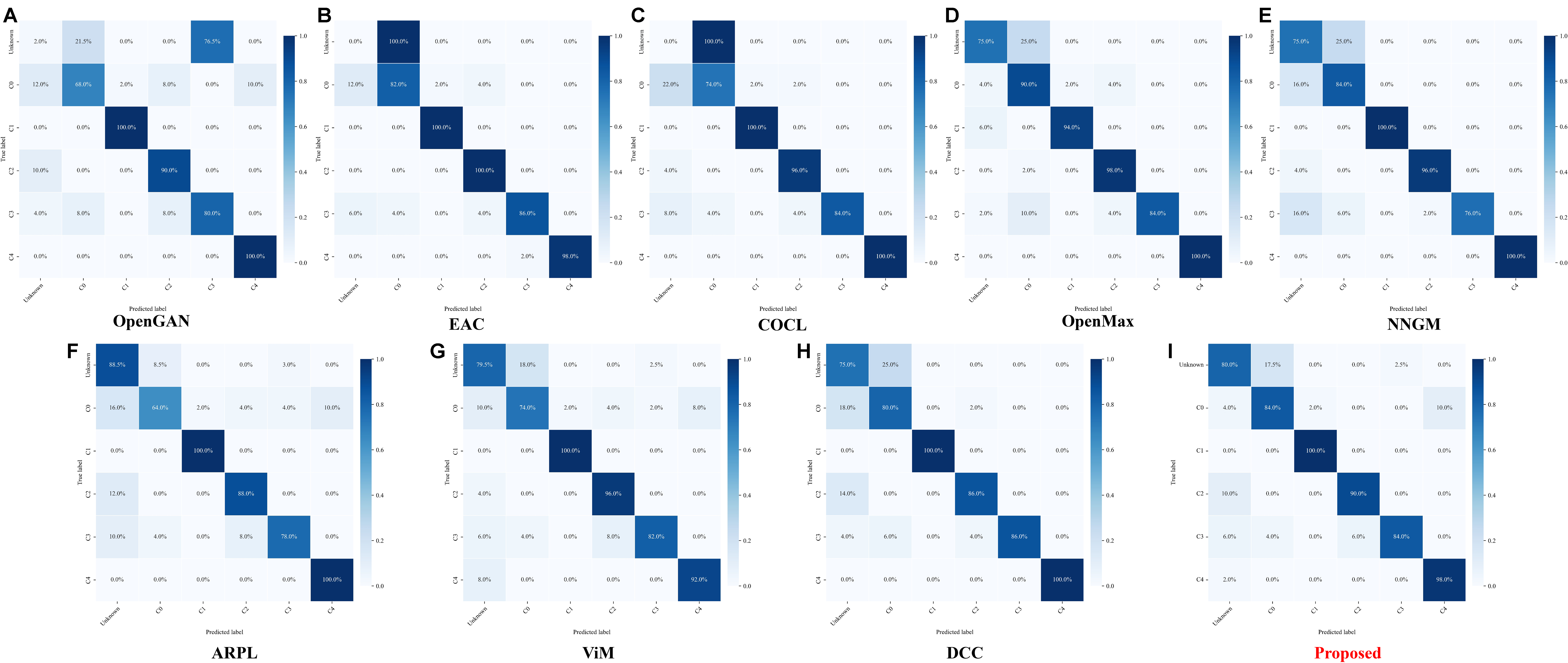
Figure 8. Confusion matrices under a representative challenging open-set task. The representative task corresponds to Task 5 in Table 3; the known classes C0, C2, C3, C4, and C8 are displayed using task-local labels C0-C4, while the unknown class combines C1, C5, C6, and C7. The proposed method exhibits the clearest diagonal structure and the strongest unknown-class recognition, indicating improved separation between known and unknown samples.
As shown in Figure 9, the challenging setting revealed substantial differences in the feature-space structure learned by the competing open-set methods. Several baseline methods exhibited varying degrees of overlap between known and unknown samples, particularly around the most confusable regions, indicating that their learned representations did not fully separate unknown instances from nearby known classes. In contrast, the proposed method produced a visibly cleaner organization of the embedding space, with known samples forming more compact clusters and unknown samples occupying more distinct regions with reduced intrusion into the major known-class groups. Although limited local proximity between known and unknown samples was still present in a few boundary regions, the overall separation pattern was clearer than that of the competing baselines. This qualitative result is consistent with the confusion matrices and quantitative open-set metrics, and suggests that the proposed method improves feature-level discriminability under difficult open-set conditions.
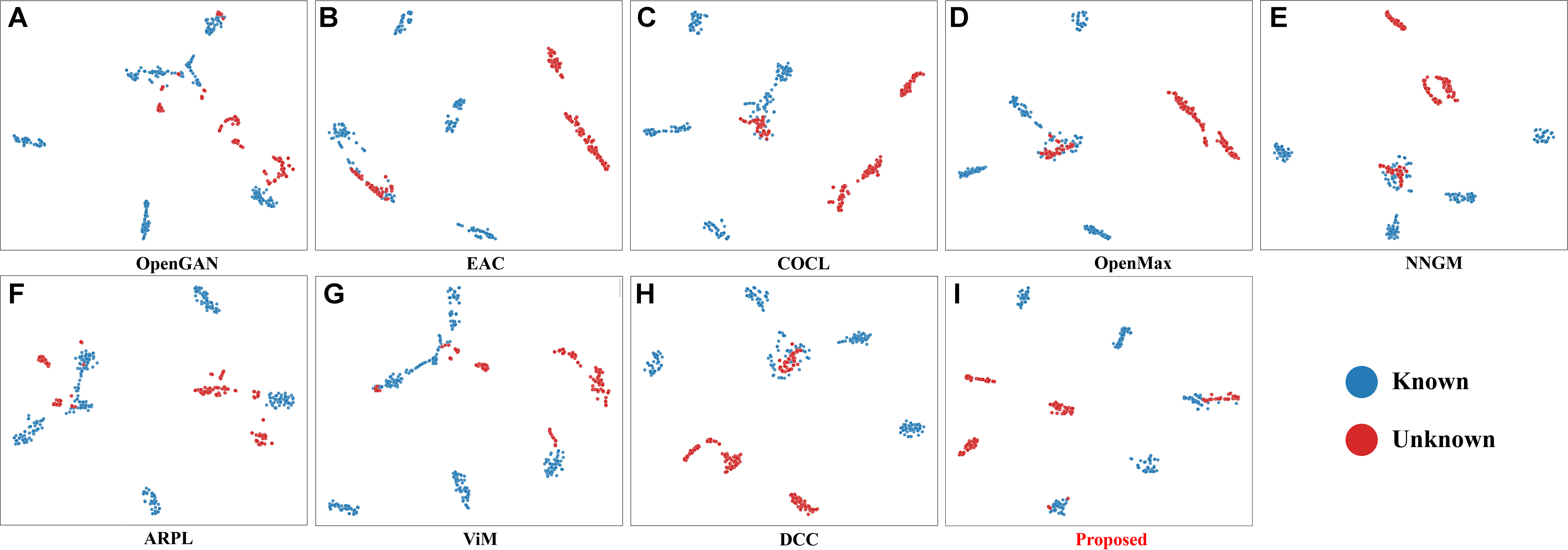
Figure 9. t-SNE visualization of feature embeddings under a representative challenging open-set task. The proposed method yields more compact known-class clusters and clearer separation between known and unknown samples than competing methods. t-SNE: Distributed stochastic neighbor embedding.
A closer inspection of the failure cases indicates that the remaining errors are mainly concentrated near electrically related known classes, especially C1 and C2 in the representative challenging task. These classes correspond to lure-lamp and metal-mesh open-circuit faults, whose current-voltage signatures can be similar to those of some unknown abnormal states when illumination fluctuation, unstable power supply, or load variation changes the operating signal. Therefore, the residual misclassification of unknown samples is physically plausible: unknown faults with similar electrical responses may fall near the acceptance regions of known electrical faults. Compared with the baseline methods, the proposed framework reduces this leakage by forming more compact known-class clusters and applying class-adaptive rejection thresholds, but a small number of boundary samples remains difficult to separate.
5. DISCUSSION
These results can be interpreted in relation to prototype-based open-set recognition, Mahalanobis-distance-based metrics, class-wise thresholding, and conformal calibration. Classical Mahalanobis distance and class-wise thresholding provide useful distance normalization and class-dependent decision boundaries, but they are often used as post-hoc decision rules. In contrast, the proposed framework couples dispersion-aware prototype matching with known-only conformal threshold calibration. It also differs from generalized zero-shot fault diagnosis methods using auxiliary sets, which aim to recognize unseen classes by transferring auxiliary semantic or fault-related information. In the present open-set setting, unknown fault classes and auxiliary unknown-class information are unavailable during training and threshold tuning; therefore, the objective is reliable unknown-fault rejection rather than explicit unseen-class recognition.
The ablation results in Table 5 show that the gains of the full model arise from the complementary effects of UAPD and CACT. UAPD contributes to the metric side by normalizing prototype matching with class-wise feature dispersion, whereas CACT contributes to the rejection side by calibrating class-specific thresholds from known calibration samples. This distinction is most evident in Task 5, where removing UAPD increased OS′ but substantially reduced UNK and H-score, indicating a shift toward known-class bias. These results suggest that the proposed method is not simply a combination of a Mahalanobis-like distance and class-wise thresholds, but a unified open-set decision framework adapted to class-dependent latent-space geometry.
The role of CACT further illustrates the trade-off between known-class recognition and unknown-fault rejection. In Task 3 and Task 5, removing CACT led to higher UNK or H-score in some cases, but it did not surpass the full model in OS. This indicates that more aggressive rejection can improve one metric while weakening the overall decision balance. CACT therefore mainly improves the stability of the open-set operating point, rather than uniformly maximizing unknown rejection in every task.
The qualitative results are consistent with this interpretation. The confusion matrices in Figure 8 show that the main errors occur near the boundary between unknown samples and confusable known classes. The distributed stochastic neighbor embedding (t-SNE) visualization in Figure 9 further shows that the proposed method forms more compact known-class clusters and clearer known/unknown separation than the competing baselines. These observations suggest that the improvement is supported not only by threshold calibration, but also by a more structured latent representation.
From an application perspective, the proposed framework is relevant to field-deployed SIL-IoTs systems, where new fault modes may emerge because of component aging, environmental disturbance, maintenance inconsistency, or device replacement. A closed-set model may incorrectly force such samples into known classes. By combining discriminative representation learning, class-wise prototype distance, and known-only threshold calibration, the proposed method provides a practical strategy for open-set fault diagnosis in the present SIL-IoTs setting.
6. LIMITATIONS
Several limitations should be acknowledged. First, the experimental validation is based on a single SIL-IoTs dataset containing nine fault categories. Although the five open-set tasks evaluate different known/unknown class partitions, they are still constructed from the same underlying data source and electrical-signal modality. Therefore, the present results should be interpreted as evidence for the effectiveness of the proposed framework in the current SIL-IoTs diagnosis setting, rather than as a complete demonstration of general applicability across different agricultural IoT platforms, sensor modalities, or larger fault taxonomies.
Second, the validity of CACT relies on the approximate exchangeability assumption of conformal calibration. Specifically, the known-class calibration samples and future deployment samples are expected to follow the same or a sufficiently stable distribution after preprocessing and feature extraction. Under this condition, the class-specific conformal thresholds can provide meaningful known-class acceptance boundaries at the prescribed risk level. However, seasonal variation, sensor drift, component aging, maintenance inconsistency, and changes in deployment conditions may weaken this assumption. Therefore, fixed offline thresholds may require periodic updating or online recalibration in long-term agricultural IoT deployment.
Third, the current framework operates at the window level and estimates prototypes, variances, and thresholds offline. This may limit its responsiveness to gradual distribution shifts or newly evolving fault patterns. Although the proposed method improves open-set robustness, its advantage is not uniform across all individual metrics, as reflected by OS′ in Task 5 and H-score in Task 3. This suggests that the balance between known-class recognition and unknown-fault rejection still depends on task difficulty and latent-space geometry. Future work will extend the framework to larger multi-device datasets, incorporate richer environmental and operational information, and investigate online recalibration strategies for updating prototypes, variances, and class-adaptive thresholds over time.
7. CONCLUSIONS
This article addressed open-set fault diagnosis for SIL-IoTs systems by proposing a prototype-based diagnosis framework that combines discriminative representation learning, UAPD, and CACT. The central idea is to perform open-set decision-making in a prototype-centered latent space while explicitly accounting for class-wise feature dispersion and class-specific acceptance boundaries. In this way, the proposed framework improves not only known-fault classification but also the reliable rejection of previously unseen fault conditions under realistic field deployment settings.
Experimental results across five open-set diagnosis tasks showed that the proposed method consistently achieved the highest open-set overall accuracy and delivered strong H-score performance in most cases, indicating a stable balance between known-class recognition and unknown-fault rejection. The ablation results further confirmed that UAPD and CACT play complementary roles: UAPD improves prototype-matching fidelity under unequal class compactness, whereas CACT stabilizes class-dependent rejection behavior without relying on real unknown samples during threshold tuning. The confusion-matrix and t-SNE analyses provided additional qualitative evidence that the proposed framework improves both class-wise separability and feature-level organization in challenging open-set conditions.
These findings suggest that prototype-based open-set diagnosis is a promising direction for the current SIL-IoTs diagnosis setting and may provide a useful basis for broader intelligent agricultural equipment monitoring after further validation. However, the current evidence is limited to a single SIL-IoTs dataset and one electrical-signal modality, and thus should not be interpreted as a complete demonstration of general applicability across agricultural IoT platforms. Future work will extend the framework to cross-device, cross-season, and cross-domain open-set diagnosis scenarios, incorporate larger and more diverse fault taxonomies, explore multimodal diagnosis using environmental and operational information, and investigate online recalibration strategies that update prototypes and rejection thresholds as operating conditions evolve.
DECLARATIONS
Authors’ contributions
Made substantial contributions to conception and design of the study and performed data analysis and interpretation: Wang, Z.; Yang X.
Performed data acquisition, as well as provided administrative, technical, and material support: Zhou X.; Guo X.
Availability of data and materials
The primary dataset is deposited at Mendeley Data: https://dx.doi.org/10.17632/dr3wny675w.1.
AI and AI-assisted tools statement
During manuscript preparation, the authors used the AI tool ChatGPT (version GPT-6 Astra, released 2026-09-03) for language polishing and improving clarity. The AI tool Gemini (version Gemini 3 Pro Image Preview, released 2025-11-20) was used to generate the background scene and the illustration in the “Challenge definition” section of the graphical abstract. The photographs of the SIL-IoTs equipment were taken by the authors. All AI-assisted outputs were reviewed, verified, and edited by the authors, who take full responsibility for the final published work. No AI tools were used to generate experimental data or determine the research conclusions.
Financial support and sponsorship
This research was funded in part by the National Natural Science Foundation of China (Grant 62402003), in part by the Anhui Science and Technology University Talent Introduction Project (Grant RCYJ202402), and in part by the University-level Interdisciplinary Project (Grant XK-XJJC002).
Conflicts of interest
All authors declared that there are no conflicts of interest.
Ethical approval and consent to participate
Not applicable.
Consent for publication
Not applicable.
Copyright
© The Author(s) 2026.
REFERENCES
1. Mansoor, S.; Iqbal, S.; Popescu, S. M.; Kim, S. L.; Chung, Y. S.; Beak, J. H. Integration of smart sensors and IOT in precision agriculture: trends, challenges and future prospectives. Front. Plant. Sci. 2025, 16, 1587869.
2. Peng, W.; Liu, Z.; Cai, J.; Zhao, Y. Research and application progress of electronic ear tags as infrastructure for precision livestock industry: a review. Intell. Robot. 2025, 5, 433-49.
3. Ge, C.; Zhang, G.; Wang, Y.; Shao, D.; Song, X.; Wang, Z. Research status and development trends of artificial intelligence in smart agriculture. Agriculture 2025, 15, 2247.
4. Yang, X.; Shu, L.; Li, K.; Huo, Z.; Shu, S.; Nurellari, E. SILOS: an intelligent fault detection scheme for solar insecticidal lamp IoT with improved energy efficiency. IEEE. Internet. Things. J. 2023, 10, 920-39.
5. Ejiyi, C. J.; Cai, D.; Thomas, D.; et al. Comprehensive review of artificial intelligence applications in renewable energy systems: current implementations and emerging trends. J. Big. Data. 2025, 12, 169.
6. Kong, Z.; Xu, X.; Jin, X.; Ji, C.; Zhang, Z.; Que, Z. A deep evidence mining approach for trustworthy open-set fault diagnosis of rotating machinery. Appl. Soft. Comput. 2026, 186, 114142.
7. Kopton, J.; de Bruin, S.; Schulz, D.; Luedeling, E. Combining spatio-temporal pest risk prediction and decision theory to improve pest management in smallholder agriculture. Comput. Electron. Agric. 2025, 236, 110426.
8. Rashid, T.; Majumder, A.; Natarajan, B. Graph-based spatio-temporal soil moisture imputation with uncertainty quantification. Smart. Agric. Technol. 2026, 15, 102455.
9. Yu, X.; Zhao, Z.; Zhang, X.; et al. Deep-learning-based open set fault diagnosis by extreme value theory. IEEE. Trans. Ind. Informat. 2022, 18, 185-96.
10. Liu, M.; Cheng, Z.; Yang, Y.; Hu, N.; Shen, G.; Yang, Y. Adaptive reconstruct feature difference network for open set domain generalization fault diagnosis. Eng. Appl. Artif. Intell. 2025, 142, 109895.
11. Zhao, Z.; Yang, B. Open set recognition of intelligent bearing fault diagnosis based on hybrid neural network and improved OPENMAX. In 2024 7th International Conference on Information Communication and Signal Processing (ICICSP), Zhoushan, China. Sep 21-23, 2024. IEEE; 2024. pp. 999-1004.
12. Chen, G.; Peng, P.; Wang, X.; Tian, Y. Adversarial reciprocal points learning for open set recognition. IEEE. Trans. Pattern. Anal. Mach. Intell. 2022, 44, 8065-81.
13. Kong, S.; Ramanan, D. OpenGAN: open-set recognition via open data generation. In 2021 IEEE/CVF International Conference on Computer Vision (ICCV), Montreal, Canada. Oct 10-17, 2021. IEEE; 2021. pp. 793-802.
14. Luan, S.; Gu, Z.; Saremi, A.; Freidovich, L.; Jiang, L.; Wan, S. Timing performance benchmarking of out-of-distribution detection algorithms. J. Sign. Process. Syst. 2023, 95, 1355-70.
15. Miao, W.; Pang, G.; Bai, X.; Li, T.; Zheng, J. Out-of-distribution detection in long-tailed recognition with calibrated outlier class learning. Proc. AAAI. Conf. Artif. Intell. 2024, 38, 4216-24.
16. Ke, S.; Gao, L.; Li, X.; Gao, Y. Open-set fault diagnosis based on prototype learning with dual category-classifier. In 2024 IEEE 20th International Conference on Automation Science and Engineering (CASE), Bari, Italy. Aug 28 - Sep 01, 2024. IEEE; 2024. pp. 3201-6.
17. Ghosal, S. S.; Sun, Y.; Li, Y. How to overcome curse-of-dimensionality for out-of-distribution detection? Proc. AAAI. Conf. Artif. Intell. 2024, 38, 19849-57.
18. Wei, D.; Zuo, M.; Tian, Z. Open-set fault diagnosis for industrial rotating machines based on trustworthy deep learning. IEEE. Trans. Ind. Cyber. Phys. Syst. 2025, 3, 181-9.
19. Fu, Y.; Liu, Z.; Wang, Z. Logit prototype learning with active multimodal representation for robust open-set recognition. Sci. China. Inf. Sci. 2024, 67, 162204. https://files.sciengine.com/pdfs/1674-733X/143FD78723854C9F9A8444E33ECE9AF1.pdf. (accessed 2026-10-22).
20. Dong, Y.; Li, Y.; Xu, M.; Wang, R. Data generation and prototype learning based open-set fault diagnosis for rotating machinery. In 2024 Prognostics and System Health Management Conference (PHM), Stockholm, Sweden. May 28-31, 2024. IEEE; 2024. pp. 202-8.
21. Ning, P.; Shi, X.; Holderbaum, W.; Xiong, W. Multiclassifier-weighted adversarial network-based open-set fault diagnosis for multimode chemical processes. IEEE. Sens. J. 2026, 26, 8448-59.
22. Shi, Y.; Ghosh, S.; Belkhouja, T.; Doppa, J. R.; Yan, Y. Conformal prediction for class-wise coverage via augmented label rank calibration. In Advances in Neural Information Processing Systems. vol. 37. Curran Associates, Inc.; 2024. pp. 132133-78.
23. Tang, H.; Jing, W.; Tang, D.; Yang, Z.; Yang, X.; Xie, W. Global-local attention-aware zero-shot learning for industrial fault diagnosis. IEEE. Trans. Instrum. Meas. 2025, 74, 1-16.
24. Assefa, M.; Naseer, M.; Ganapathi, I. I.; Ali, S. S.; Seghier, M. L.; Werghi, N. DyCON: dynamic uncertainty-aware consistency and contrastive learning for semi-supervised medical image segmentation. In 2025 IEEE/CVF Conference on Computer Vision and Pattern Recognition (CVPR), Nashiville, USA. Jun 10-17, 2025. IEEE; 2025. pp. 30850-60.
25. Jian, C.; Peng, Y.; Mo, G.; Chen, H. Open-set domain generalization for fault diagnosis through data augmentation and a dual-level weighted mechanism. Adv. Eng. Inform. 2024, 62, 102703.
26. Yu, X.; Zhao, Z.; Zhang, X.; Chen, X.; Cai, J. Statistical identification guided open-set domain adaptation in fault diagnosis. Reliab. Eng. Syst. Saf. 2023, 232, 109047.
27. Liu, B.; Chen, Y.; Liu, S.; Kim, H. S. Deep learning in latent space for video prediction and compression. In 2021 IEEE/CVF Conference on Computer Vision and Pattern Recognition (CVPR), Nashville, USA. Jun 20-25, 2021. IEEE; 2021. pp. 701-10.
28. Wang, B.; Wen, L.; Li, X.; Gao, L. Adaptive class center generalization network: a sparse domain-regressive framework for bearing fault diagnosis under unknown working conditions. IEEE. Trans. Instrum. Meas. 2023, 72, 1-11.
29. Miller, D.; Sunderhauf, N.; Milford, M.; Dayoub, F. Class anchor clustering: a loss for distance-based open set recognition. In 2021 IEEE Winter Conference on Applications of Computer Vision (WACV), Waikoloa, USA. Jan 03-08, 2021. IEEE; 2021. pp. 3569-77.
30. Wang, C.; Cheng, B.; Deng, L. An adaptive thresholding approach for open set fault diagnosis. Meas. Sci. Technol. 2024, 36, 016177.
Cite This Article
 Open Access
How to Cite
Wang, Z.; Yang, X.; Zhou, X.; Guo, X. Open-set fault diagnosis for solar insecticidal lamp IoT systems using adaptive prototypes. Intell. Robot. 2026, 6(4), 843-67. https://dx.doi.org/10.20517/ir.2026.37
Download Citation
If you have the appropriate software installed, you can download article citation data to the citation manager of your choice. Simply select your manager software from the list below and click on download.
Export Citation File
Type of Import
Tips on Downloading Citation
Citation Manager File Format
Type of Import
Direct Import: When the Direct Import option is selected (the default state), a dialogue box will give you the option to Save or Open the downloaded citation data. Choosing Open will either launch your citation manager or give you a choice of applications with which to use the metadata. The Save option saves the file locally for later use.
Indirect Import: When the Indirect Import option is selected, the metadata is displayed and may be copied and pasted as needed.
About This Article
Copyright

Data & Comments
Data
0










Comments
Comments must be written in English. Spam, offensive content, impersonation, and private information will not be permitted. If any comment is reported and identified as inappropriate content by OAE staff, the comment will be removed without notice. If you have any queries or need any help, please contact us at [email protected].