

Container-surface-guided dual-task learning for defect detection in complex port scenes
 0
 ,
Graphical Abstract
Abstract
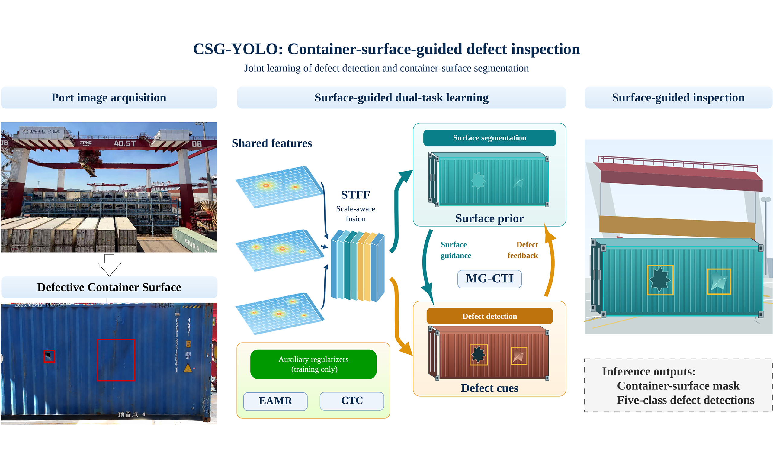
Automatic container defect inspection in complex port environments is hindered by substantial scale variation and defect-like interference from non-container regions. This article presents CSG-YOLO, a container-surface-guided dual-task framework that jointly learns five-class defect detection and container-surface segmentation. Its scale-tuned feature fusion module adapts multi-level neck features to defects of different spatial extents, while mask-guided cross-task interaction bidirectionally exchanges the learned surface prior and defect cues between the task heads. Center-to-container consistency and edge-aware mask refinement losses respectively encourage defect-center coverage and surface-boundary consistency. On a single-terminal dataset of 4,000 distinct port images containing 4,480 defect instances, CSG-YOLO-N achieves mean scores of 58.1 average precision (AP), 93.0 AP50, and 65.0 AP75 across three independent training runs, with 16.3 GFLOPs. Compared with YOLOv12-N, it improves these metrics by 2.4, 3.2, and 4.1 points, respectively, while reducing mean overall missed detection rate from 6.4% to 5.7%, false positives per image from 0.19 to 0.11, and outside-region-of-interest (ROI) detection ratio from 1.8% to 0.2%. It also obtains a mean Surface intersection over union of 76.7%. These results support the effectiveness of explicit container-surface modeling for defect detection and suppression of spatially invalid detections on the evaluated dataset. Generalization to other port environments remains to be established.
Keywords


 Download PDF
1. INTRODUCTION
1.1. Background and related works
Containers are essential carriers in global logistics and are routinely handled during terminal loading and unloading, yard stacking, gate transfer, and sea–land intermodal transportation. Frequent turnover and complex port operations expose container bodies to collisions, compression, friction, and environmental contamination, resulting in defects such as deformation, holes, post damage, repair patches, and surface contamination. These defects can compromise structural integrity and sealing performance, increasing the risk of cargo loss, contamination, and transportation accidents.
Container defect inspection in ports still relies heavily on manual visual examination, which is labor-intensive, subjective, and difficult to sustain under long-duration, high-throughput operation. Reliable automatic detection is therefore important for improving the efficiency and consistency of intelligent container inspection.
The development of automated terminals has made computer vision an important component of intelligent port perception. Deep learning detectors have been studied for container-terminal perception tasks[1], including lightweight container detection using YOLOv5s[2]. Earlier work used template matching to identify markings and other objects on side-view container images as a step toward damage inspection[3]. Deep learning studies have formulated damage assessment as damaged-versus-undamaged image classification[4], investigated Vision Transformer-based container inspection[5], and developed a convolutional neural network (CNN)–Transformer hybrid for appearance-defect classification[6]. Image-level classification does not provide defect bounding boxes, motivating explicit localization for automated inspection.
Container-damage detection studies have explored several detector designs. Huang et al. proposed an attention-enhanced YOLO framework for port environments[7], Zhao incorporated C2PSA into YOLOv11[8], and Zheng et al. combined gated feature interaction, a high-resolution detection layer, and attention in an improved YOLOv8 detector[9]. Bahrami et al. investigated anchor-box optimization for container corrosion inspection[10], while YOLO-NAS has been applied to container-damage detection[11]. Zhang investigated self-contrastive learning with deep CNNs for container-damage detection[12]. Vasileiadis et al. combined container tracking and damage detection during crane unloading[13], whereas Rahman et al. applied RF-DETR to container-damage detection in ports[14]. In the present inspection setting, defect-like textures on ground areas, spreaders, shadows, and other non-container structures motivate explicitly modeling the valid supporting surface.
Compared with bounding-box detection, segmentation provides pixel-level region representations and has also been explored for container inspection. Li et al. developed an fully convolutional network (FCN)-based damage-identification network with pyramid pooling and fusion upsampling[15]. Wang et al. developed a lightweight SOLO-based design combining GC-ShuffleNetV2, an improved path aggregation feature pyramid network (PAFPN), and a decoupled SOLO head[16]. Su and Yu proposed a YOLO11-based end-to-end detection and segmentation model for container-surface damage[17]. Ornelas
Related scale-adaptive designs have also been studied in other dense-prediction tasks. SANet combines scale-adaptive feature extraction and multi-scale aggregation for lightweight salient object detection[19]. This work provides context for scale adaptation rather than container-defect benchmark results.
Industrial surface inspection has also used segmentation to support defect decisions. Božič et al. combine pixel-level defect segmentation with image-level classification to learn from mixed weak and full supervision[20]. Their segmentation target is the anomalous region, and the decision concerns whether an image contains a defect. CSG-YOLO instead learns the supporting container surface, including normal and damaged portions, as a common spatial prior for multi-class bounding-box detection. This difference concerns the supervised representation and its use in localization, rather than the general idea of coupling segmentation with another inspection task.
Joint prediction and cross-task information transfer are established ideas. Mask R-CNN[21] predicts object-instance masks alongside bounding boxes, while PAD-Net[22] uses intermediate auxiliary predictions and multi-modal distillation for depth estimation and scene parsing. These precedents motivate a more specific distinction in container inspection: the segmentation target and its role in detection. In the standard Mask R-CNN formulation, masks and boxes describe the same object instances; using a supporting container surface to guide a different set of defect instances requires a distinct auxiliary target and a corresponding transfer mechanism. Here, the segmentation target is the valid container surface, including both defective and non-defective portions, rather than the pixels of individual defect categories. Its predicted representation supplies a shared spatial prior for all five defect classes. The methodological focus is how this inspection-domain prior conditions dense detection features, receives complementary defect cues, and is supervised for spatial consistency.
Accordingly, three challenges remain in real-world container defect detection.
• Images captured at quay cranes, gates, and yards contain vehicles, ground areas, spreaders, locking devices, shadows, reflections, and buildings. These non-container regions may resemble true defects and induce background false positives.
• Defect instances vary substantially in area, morphology, and appearance. Small instances may lose fine spatial cues during deep feature extraction, whereas spatially extended instances require broader context and stable boundary representation. This variation occurs both within and across semantic categories.
• Existing methods primarily model the defects themselves and rarely use the valid container surface as an explicit prior, leaving the spatial consistency of predicted defects insufficiently constrained.
1.2. Main contributions
CSG-YOLO is a container-surface-guided multi-task framework for practical port inspection, with defect detection as its primary task and surface segmentation as auxiliary spatial guidance. Its methodological contribution is the explicit coupling of the supervised surface representation with detection: the learned prior modulates multi-scale detection features, and detached defect responses refine the surface-mask prototype through a complementary path. Center-to-container consistency (CTC) and edge-aware mask refinement (EAMR) objectives supervise the prior at annotated defect centers and surface boundaries, linking defects to their supporting surface.
The framework adopts the YOLO detection architecture and uses established convolution, attention, and residual-gating operations. Joint training, bidirectional information exchange, and these individual operators are not claimed as new principles. The proposed design specifies the surface-prior representation, its transfer within the dual-task head, and the associated consistency supervision. Scale-tuned feature fusion (STFF) provides complementary scale-level feature modulation upstream of this interaction; its feature-derived gates do not receive segmentation predictions.
The main contributions of this article are summarized as follows.
• We formulate container-surface segmentation as learning a common inspection-domain prior for five-class defect detection. Mask-guided cross-task interaction (MG-CTI) transfers this prior to detection features through residual spatial gates and returns detached defect responses to refine the surface-mask prototype within a one-stage architecture.
• We design STFF to combine explicit fusion-level embeddings, local and dilated spatial cues, and residual shared-feature modulation for defects of different spatial extents. Complementary center-to-container and edge-aware objectives supervise the learned surface prior without adding inference-time loss computation.
• We evaluate the design through comparative, scale-wise, and qualitative studies and three-run component ablations. Detection-only STFF, segmentation without explicit interaction, directional MG-CTI, and training-loss comparisons distinguish the observed contributions of feature modulation, auxiliary supervision, and surface-prior transfer on the evaluated port dataset.
The remainder of this article is organized as follows. Section 2 presents the proposed framework and its main components. Section 3 describes the experimental protocol and results. Section 4 concludes the article and outlines future work.
2. METHODS
2.1. Overall architecture and multi-task learning framework
The analysis in Section 1 indicates that container defect detection should not be formulated as an unconstrained whole-image search problem. Since real defects are expected to occur on the container surface, explicitly modeling the valid container-surface region can provide an effective spatial prior for defect localization. Based on this observation, the proposed method formulates container defect detection and container-surface segmentation as a unified multi-task learning problem, in which the segmentation branch provides surface-aware guidance for detection and the detection branch provides defect-related cues for segmentation refinement.
As shown in Figure 1, the proposed framework is built upon a YOLOv12-style one-stage architecture[23] and consists of four main components: a shared backbone, a feature pyramid network (FPN)/path aggregation network (PAN) neck enhanced by the proposed STFF module, a dual-task prediction head, and a MG-CTI module. For clarity, the complete framework is referred to as CSG-YOLO, short for Container-Surface-Guided YOLO, in the experimental tables, with the suffixes indicating different model scales. Let
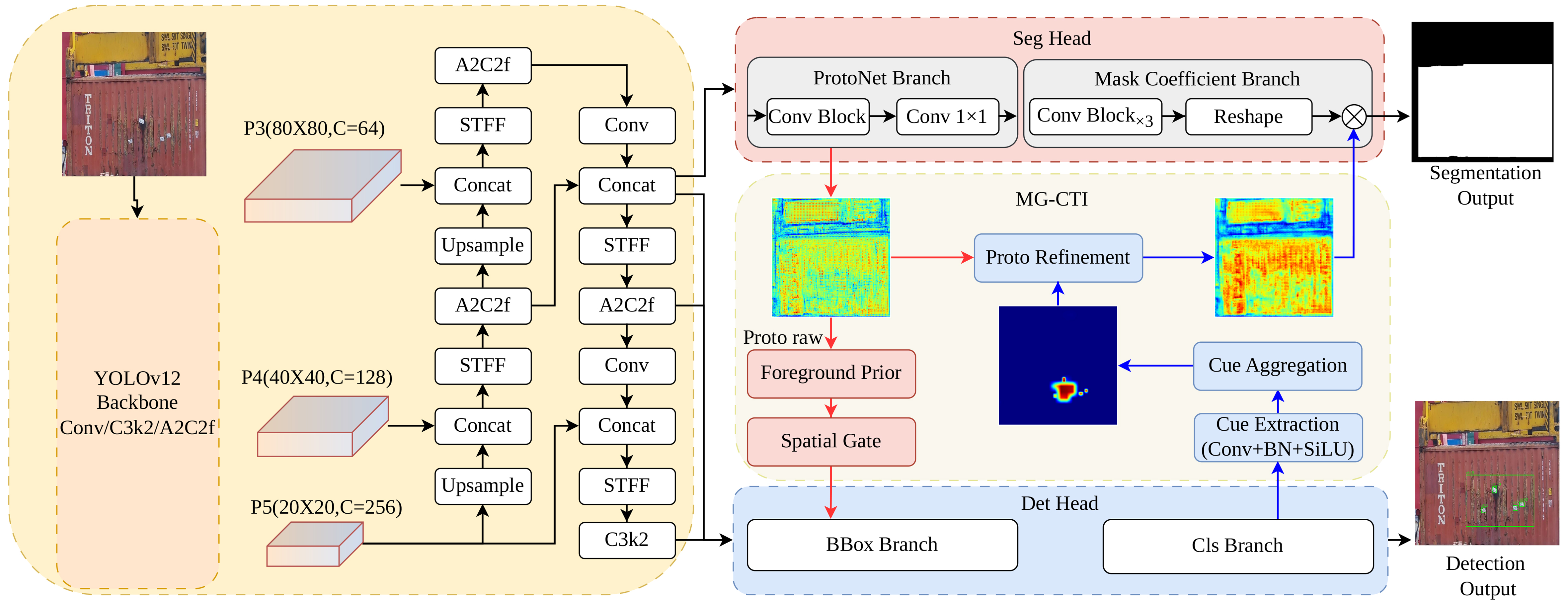
Figure 1. Overall architecture of the proposed container-surface-prior-guided dual-task network. The shared backbone and neck extract multi-scale features, while the detection and segmentation branches are connected through MG-CTI for lightweight bidirectional task interaction. The photographs in the upper-left input and lower-right detection-output panels were acquired at Qianwan Terminal, Port of Qingdao, China. All port photographs shown throughout this article share this source and are reproduced with written permission for journal publication. Detection overlays, annotations, and heatmaps were generated in this study. MG-CTI: Mask-guided cross-task interaction; STFF: scale-tuned feature fusion; Conv: convolution; BBox: bounding box; BN: batch normalization; Cls: classification; SiLU: sigmoid linear unit.
where F3, F4, and F5 denote feature maps with different spatial resolutions and semantic levels, thereby providing a unified multi-scale representation for defect localization and container-surface modeling.
On top of the shared features, the dual-task head decouples defect detection and container-surface segmentation. The detection branch predicts five-category defect bounding boxes and class scores from the multi-scale features. In parallel, the segmentation branch estimates the valid container-surface mask by generating mask prototypes from the high-resolution feature and combining them with mask coefficients predicted from the multi-scale features. This design enables the two tasks to share common visual representations while maintaining task-specific prediction parameters.
However, the two branches are not treated as independent parallel outputs. In the dual-task head, the segmentation-derived container-surface prior guides the detection features, while the detection branch returns defect-related responses to refine the segmentation prototype. STFF operates upstream in the neck and does not receive the segmentation prediction, mask prototype, or the prior generated by MG-CTI. Accordingly, the dual-task prediction process can be compactly formulated as
where P denotes the mask prototype generated by the segmentation branch, and
The two outputs describe different entities: detection predicts defect instances, while segmentation estimates their valid supporting surface. Relative to a shared-feature multi-task baseline with parallel heads, MG-CTI introduces explicit transfer of this surface representation into the detection features and complementary refinement of the mask prototype using defect responses. The prior is applied before the final detections are produced, using soft residual feature modulation rather than a binary mask applied to completed detections. At inference, the prior is predicted from image features; ground-truth surface annotations are used only for training and evaluation. The following subsections detail STFF and MG-CTI.
2.2. STFF module
Container defects vary substantially in area, morphology, and appearance, and each semantic category may contain small, medium, and large instances under the Common Objects in Context (COCO) area bins. Compact instances depend strongly on fine spatial cues, whereas spatially extended instances require broader context and stable region-level representations. STFF therefore retains local evidence while aggregating wider contextual cues. Its scale embedding identifies the fusion level, and its attention and shared-feature gates modulate the fused representation before the task-specific heads. STFF does not use a task identity or task-conditioned inputs; instead, it produces a shared feature optimized by the joint detection–segmentation objective. As illustrated in Figures 2 and 3, STFF is inserted after feature concatenation in the FPN/PAN neck.
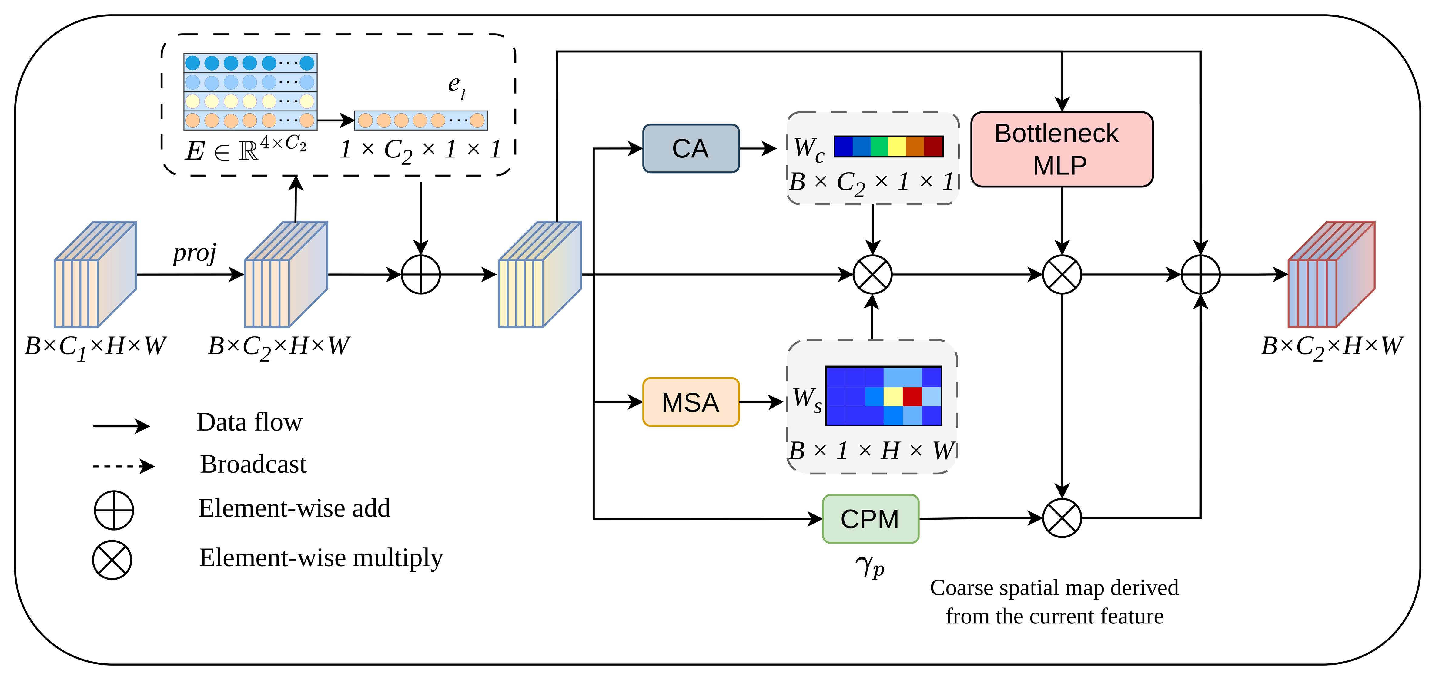
Figure 2. Data flow of the proposed STFF module, where scale embedding, channel attention, multi-receptive-field spatial attention, shared-feature gating, and feature-derived coarse spatial modulation are integrated in a residual manner. STFF: Scale-tuned feature fusion; CA: channel attention; MLP: multilayer perceptron; MSA: multi-receptive-field spatial attention; CPM: coarse spatial modulation.
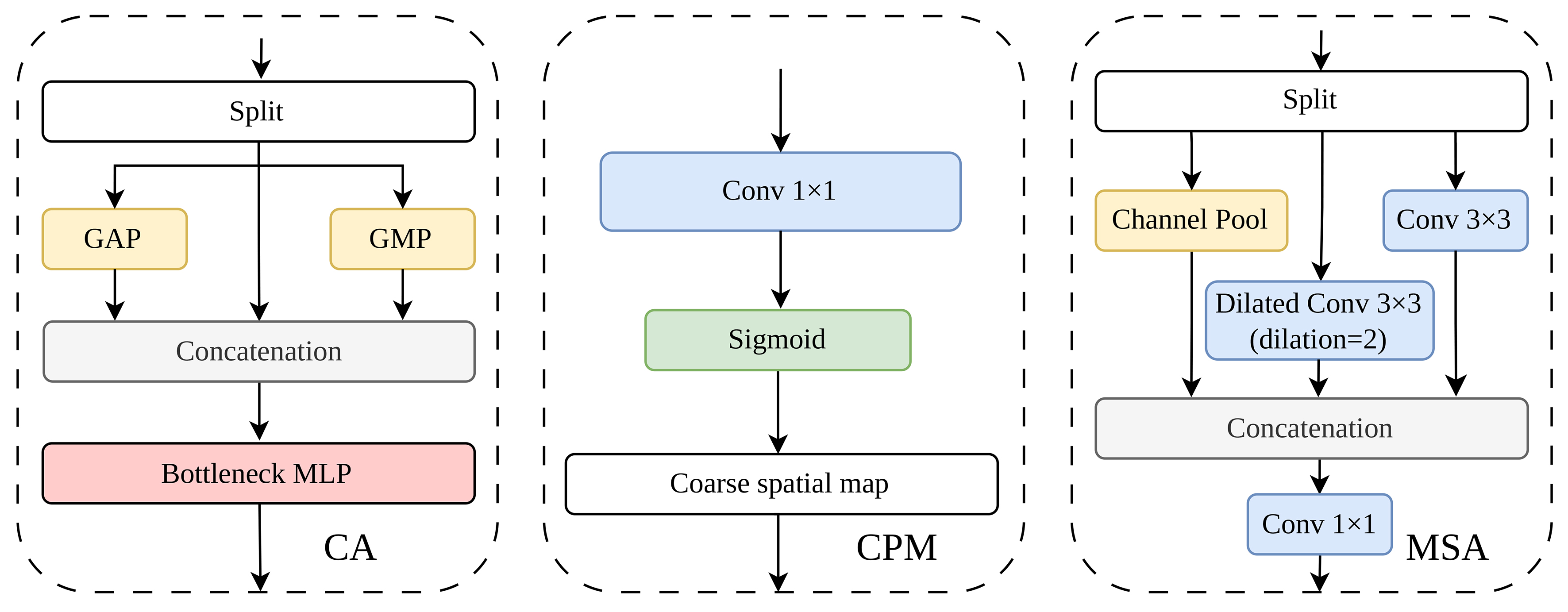
Figure 3. Main functional components of STFF, including channel attention, feature-derived coarse spatial modulation, and multi-receptive-field spatial attention. STFF: Scale-tuned feature fusion; GAP: global average pooling; GMP: global maximum pooling; MLP: multilayer perceptron; CA: channel attention; CPM: coarse spatial modulation; MSA: multi-receptive-field spatial attention; Conv: convolution.
The convolutional block attention module (CBAM)[24] sequentially derives channel and spatial attention from an intermediate feature map. STFF retains this established feature-reweighting idea but organizes it for the concatenation stages of the FPN/PAN neck: a learnable embedding identifies the fusion level, standard and dilated 3 × 3 branches provide local and wider spatial cues, and shared-feature and coarse spatial gates modulate a residual path with zero-initialized channel-wise coefficients. Compared with the backbone, pyramid, and head configuration of Fast-Solo[16], STFF is a module applied after neck concatenation rather than a replacement instance-segmentation architecture. Its scale indicator denotes the feature-fusion level, not a physical defect-size class. The output is a shared feature; no segmentation prediction enters these gates. The distinction therefore lies in the fusion-level organization and residual modulation, while the supervised surface prior and its transfer are handled separately by MG-CTI.
Let Xl denote the concatenated feature at the l-th fusion level. The channel-aligned and scale-embedded features are computed as
where ϕp(·) denotes a 1 × 1 projection or an identity mapping, and el is a learnable embedding broadcast to the spatial size of
Based solely on the scale-embedded feature X′l, the channel, spatial, shared-feature, and coarse spatial modulation weights are computed as
where GAP and GMP denote global average and maximum pooling, respectively, whereas Avgc and Maxc compute channel-wise spatial statistics. The channel mapping fc(·) uses a lightweight bottleneck transformation. The spatial mapping fs(·) combines a standard 3 × 3 convolution ϕ3(·), a dilated 3 × 3 convolution ϕd(·) with dilation 2, and channel-pooled cues to provide complementary local and contextual evidence for instances with different spatial extents. The mapping fg(·) provides a learned gate for the shared feature supplied to the subsequent dual-task head. It receives only X′l and is jointly optimized by the detection and segmentation objectives; it does not use a task identifier, a task embedding, or separate task-conditioned inputs. The 1 × 1 mapping fp(·) produces a coarse spatial modulation map directly from X′l. Importantly, Alp is an internally learned feature gate rather than a segmentation mask or an MG-CTI-derived container-surface prior; it receives no output from the segmentation head.
Finally, the residual output of STFF is computed as
where
2.3. MG-CTI module
Although STFF improves sensitivity to multi-scale cues in the neck, the spatial prior for defect localization originates from the container-surface segmentation branch. MG-CTI is therefore introduced into the dual-task head to establish lightweight bidirectional interaction. Its segmentation-to-detection path uses the learned surface prior to modulate detection features and reduce responses from non-container regions, while its detection-to-segmentation path feeds defect-related cues back to the segmentation branch to refine prototypes. This interaction improves background suppression and cross-task spatial consistency without changing the one-stage inference structure.
For the segmentation-to-detection path, MG-CTI first predicts a container-surface prior logit from the raw mask prototype and then maps it to each detection scale to generate spatial gates. The gated detection feature is computed as
where P denotes the raw mask prototype, ψq(·) denotes the container-surface-prior prediction head, Q ∈
For the detection-to-segmentation path, MG-CTI aggregates the multi-scale class responses from the detection branch into a defect-aware heat map. The response aggregation and prototype refinement are computed as
where Ci is the class-logit map of the i-th detection scale, Di denotes the corresponding defect-response map, and sg(·) denotes the stop-gradient operation. The stop-gradient operation prevents the prototype refinement path from interfering with the optimization of the detection classifier. ψr(·) denotes the prototype refinement mapping, and λr is a learnable residual coefficient initialized to zero to preserve the original prototype representation at the early training stage.
The two paths in Equations (6) and (7) assign a specific meaning to the exchanged signals. The S → D gates are derived from a supervised container-surface representation and shared across defect categories; the D → S input is a class-aggregated, stop-gradient defect-response map that refines the mask prototype. These are complementary paths within the head, without iterative alternation between complete detection and segmentation passes. The interaction does not feed segmentation predictions back into STFF, and it preserves task-specific outputs and the one-stage inference pipeline. Relative to defect-segmentation–classification coupling[20], MG-CTI exchanges a supporting-surface representation and dense defect-localization cues rather than using a defect mask for an image-level decision. Its S → D path modulates multi-scale detection features before box prediction, and its D → S path supplies detached detector class responses to prototype refinement. Gradient stopping is an established training operation; the specific design here is its placement on the returned defect-response signal, together with the distinct role of the supervised surface prior.
2.4. Loss function
The proposed network is trained with a multi-task objective that jointly optimizes defect detection, container-surface segmentation, and surface-prior regularization. Since the detection branch follows the standard one-stage YOLO-style optimization, its loss is denoted by
where λseg, λctc, and λeamr control the contributions of the segmentation loss, the CTC loss, and the edge-aware mask refinement (EAMR) loss, respectively. In the final N, S, and X models, these weights are fixed to λseg = 0.25, λctc = 0.5, and λeamr = 0.1, respectively. Uncertainty-based loss weighting is disabled, so these coefficients are not learned during training.
For the segmentation branch, the objective is to learn a reliable representation of the valid container-surface region, which serves as the container-surface prior for subsequent defect localization. The segmentation loss is defined as
where
To reinforce the spatial agreement between annotated defect centers and the learned surface prior, a CTC loss is introduced. The underlying assumption is that real container defects should be located within the valid container-surface region. Thus, the container-surface prior generated by MG-CTI is expected to produce high responses at the centers of ground-truth defect boxes. Let Q denote the container-surface prior logit and let cj = (cjx, cjy) be the center of the j-th ground-truth defect box. The CTC loss is defined as
where Nd is the number of ground-truth defect boxes, bj is the image index of the j-th box, Π(·) maps the box center to the coordinate system of the container-surface prior map, pj is the sampled prior response, and ϵ is a small constant for numerical stability. This term directly constrains the container-surface prior Q at defect-related positions and provides a more spatially consistent prior for subsequent detection guidance. Its effect on detection is indirect: the refined prior is transferred through MG-CTI to modulate detection features. CTC neither consumes detection predictions nor directly penalizes detector confidence outside the container surface.
Although CTC constrains the container-surface prior at defect-related positions, it does not explicitly impose edge-level consistency along the annotated surface boundary. To provide complementary edge-aware supervision, the EAMR loss is defined as
where M denotes the ground-truth container-surface mask resized to the resolution of Q,
Together, these objectives optimize detection accuracy and the reliability of the learned container-surface prior. The segmentation loss provides region-level supervision, CTC encourages the prior to cover annotated defect centers, and EAMR promotes boundary consistency with the ground-truth surface mask. CTC affects detection indirectly through the prior and subsequent MG-CTI feature modulation. Both CTC and EAMR are training-time regularizers and introduce no additional loss computation during inference. The distinction of these regularizers lies in their supervised target: CTC encourages positive responses of the surface prior at annotated defect centers, while EAMR aligns edges of that prior with annotated surface boundaries. They do not introduce a new box-regression objective, Sobel operator, or binary cross-entropy formulation.
3. RESULTS
The experiments evaluate three aspects of the proposed framework. First, comparisons with representative detectors assess detection accuracy and inference efficiency. Second, full-test-set false-positive and ROI-based analyses examine the suppression of invalid detections from non-container regions. Third, category-wise, scale-wise, and ablation studies analyze the contributions of STFF, MG-CTI, and the training objectives.
3.1. Dataset
The experiments use a private container defect dataset comprising 4,000 distinct still images acquired by quay-crane cameras at Qianwan Terminal, Port of Qingdao, China. The images were obtained from the cooperating port with permission for research use and are subject to the applicable data-use and port-related confidentiality agreements. The authors selected and annotated these images from approximately 200,000 usable container-defect images acquired by this system over a two-year period. The data do not contain frames extracted from continuous videos or burst sequences and therefore include neither temporally adjacent frame pairs nor repeated video frames. The original 1,920 × 1,080 images cover diverse operating conditions, including complex backgrounds, occlusions, shadows, reflections, container textures, characters, and non-container structures. Defect instances are annotated with bounding boxes, and container-surface masks are available for all 4,000 images. During training and inference, each image is letterbox-resized to 640 × 640 with its aspect ratio preserved, and the bounding-box and mask annotations are transformed accordingly.
Both defect bounding boxes and container-surface masks were manually annotated using Labelme by three research assistants. Image screening and defect identification followed the operational container-damage assessment criteria provided by the Business Department of the Port of Qingdao, with guidance from experienced tallying personnel. Annotation quality was reviewed daily: the team leader examined every image annotated that day, checked the defect-box and surface-mask annotations, and provided feedback for correction. The annotators revised the annotations in response to this feedback. This workflow combined business-defined damage criteria, expert guidance, and daily image-by-image review to support annotation consistency.
The acquisition procedure did not repeatedly capture the same physical container or near-identical views of the same inspection event. Together with manual screening and annotation, this procedure ensured that the curated dataset contained no repeated observations of the same physical container. The curated images were then randomly divided into training and test sets at an 8:2 ratio, yielding 3,200 training images and 800 test images. Consequently, no physical container is represented in both subsets, and the training and test sets are independent at the container level. This fixed split is used in all comparative and ablation experiments. Both subsets originate from the same terminal; container-level independence therefore does not imply evaluation on an unseen port or entirely different inspection environments.
During manual selection from the larger collection, particular attention was paid to retaining examples of less frequent defect categories to improve their representation in the annotated dataset. This selection-stage effort aimed to reduce underrepresentation but did not produce a balanced class distribution. The remaining imbalance is explicitly documented by the category counts below, and its implications are examined using the category-wise average precision (AP) results reported below.
No explicit class-imbalance compensation was used during training: there was no minority-class oversampling, class-balanced sampling, or additional class-weighted loss. The effort to retain less frequent categories was confined to dataset selection.
The original engineering labels are reorganized into five defect categories for detection evaluation: Deformation, Hole, Post Damage, Repair Patch, and Contamination. The corresponding instance counts are 2,364, 1,236, 483, 211, and 186, respectively, for a total of 4,480 annotated defect instances. Since an image may contain more than one defect, the total number of annotated instances can exceed the number of images. To reflect the spatial characteristics of container defects, these categories are further described using region-aware subtypes. Specifically, Deformation includes Door Deformation and Side Deformation; Hole includes Door Hole, Side Hole, and Roof Hole; Post Damage corresponds to Corner Post Damage; Repair Patch consists of Side Repair Patch and Roof Repair Patch; and Contamination includes Door Contamination and Side Contamination. This five-category protocol is used consistently in all detection-related experiments. These labels encode semantic defect types rather than object scales and are independent of the COCO area bins for small, medium, and large instances; instances from any semantic category may fall into any of the three area ranges.
Figure 4 presents ten manually selected images to illustrate variation in defect appearance, scale, and acquisition conditions, together with the corresponding ground-truth annotations. The repair patches in the first, third, and fourth images of the top row range from small localized patches to an elongated repaired region, illustrating intra-class scale and shape variation. The second top-row image and the bottom row show holes with different sizes and contours; the first bottom-row image contains holes of several sizes within one view. Deformation and contamination annotations provide additional examples of semantic defect categories. The scenes also include backgrounds with colors similar to the container, nearby light sources, the ground, quay-crane supports, and container trucks. Machinery close to or partly obscuring the container boundary, particularly in the top-right image, illustrates the visibility challenges encountered during handling.
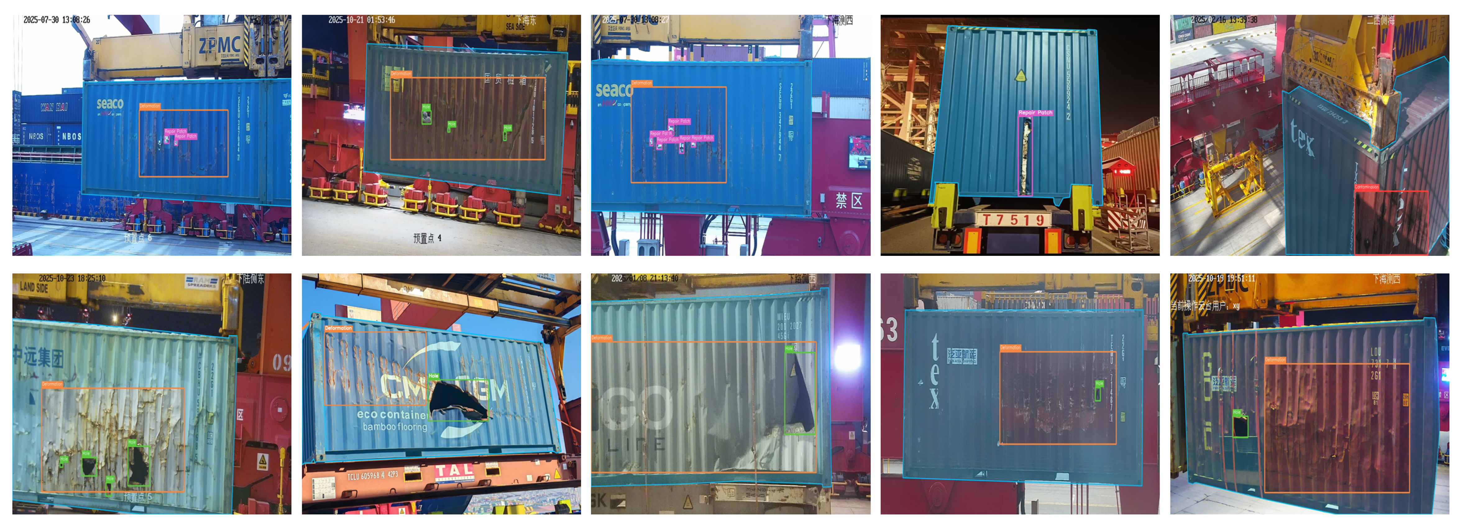
Figure 4. Ten illustrative images from the private container defect dataset with ground-truth annotations, arranged in two rows of five. Cyan contours indicate container-surface mask boundaries; colored rectangles indicate defect annotations (orange: Deformation; green: Hole; magenta: Repair Patch; red: Contamination). The examples show variation in defect scale and shape, illumination, viewpoint, and background clutter. They are selected illustrations rather than a statistically representative sample.
The cyan contours in Figure 4 trace the ground-truth container-surface mask boundaries, while the colored rectangles mark annotated defect instances. These overlays show how the surface annotation distinguishes the container region from surrounding equipment and background structures. The images were selected to illustrate these conditions rather than sampled to estimate their prevalence; they do not constitute a statistically representative subset or establish detection performance. The full category distribution is reported separately in Figure 5.
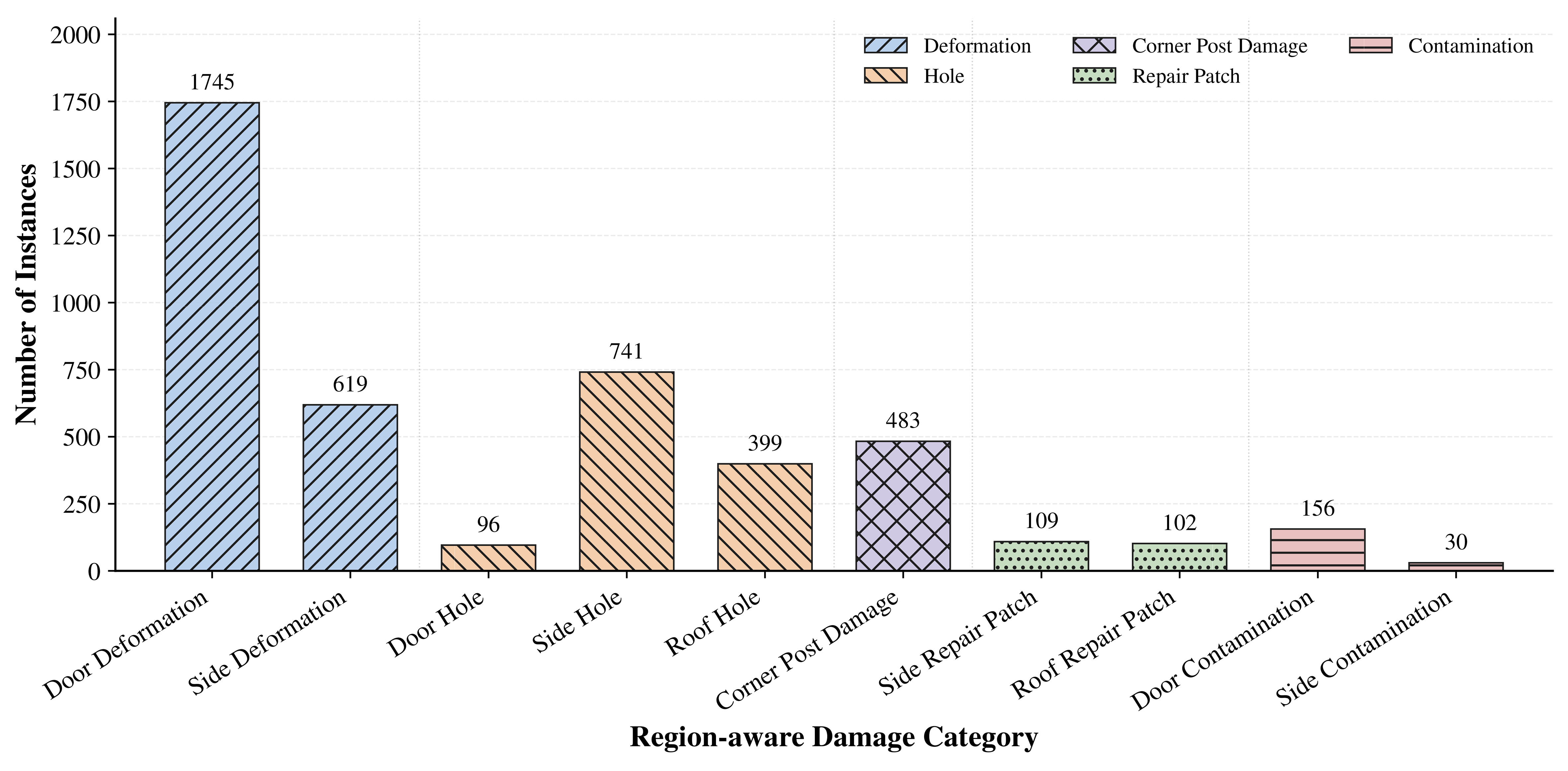
Figure 5. Region-aware defect label distribution of the container defect dataset.
As shown in Figure 5, the region-aware label distribution reports the number of instances for each subtype, with consistent colors and patterns indicating the corresponding five major defect categories.
3.2. Evaluation metrics
Defect detection is evaluated using the official COCO evaluation protocol[25]. AP denotes mean average precision over ten intersection over union (IoU) thresholds from 0.50 to 0.95 in increments of 0.05, while AP50 and AP75 are computed at fixed IoU thresholds of 0.50 and 0.75. Scale-wise APs, APm, and APl use the original-image bounding-box area A and the standard pycocotools areaRng bins: small over [0, 322], medium over [322, 962], and large from 962 upward. Endpoint handling follows the implementation, which includes the shared boundary values in adjacent ranges. The corresponding scale-wise average recall (AR) values, ARs, ARm, and ARl, are also reported. The 640 × 640 letterbox transformation is used only for model input and geometric mapping and does not redefine the area bins, which remain independent of the five semantic defect categories.
The dataset exhibits both inter-class and intra-class scale variation: defects from different semantic categories, as well as instances within the same category, can occupy substantially different image areas. Such variation reflects differences in actual defect extent, imaging distance, viewpoint, and position on the container surface. Accordingly, the COCO area bins provide standardized image-space evaluation intervals for cross-scale detection capability, rather than engineering categories with fixed physical dimensions. Even at the original 1,920 × 1,080 resolution, the pixel-area thresholds do not imply a one-to-one correspondence with physical defect sizes in container inspection.
Port inspection requires locating physical defects and limiting background alarms. Class-agnostic overall missed detection rate (OMD) and false positives per image (FPPI) assess these operational requirements, complemented by outside-ROI detection ratio (ODR) for spatial consistency and class-aware AP for detection quality. The OMD is defined as the following instance-level, class-agnostic metric:
where Nalldef is the total number of ground-truth defect instances and Nmissdef is the number that remain unmatched. Confidence-ranked predictions are greedily matched to ground-truth boxes one-to-one at IoU ≥ 0.50, with each prediction and instance matched at most once. Matching is class-agnostic because the engineering objective is to determine whether a physical defect region is localized. OMD is computed from final post-non-maximum suppression (NMS) detections at the fixed confidence threshold τ = 0.25 and should not be interpreted as an image-level complete-miss rate.
Model complexity and inference efficiency are also important for quay-crane-side inspection. Parameter count, floating-point operations (FLOPs), and per-image latency are therefore reported with the COCO metrics to assess storage cost, computational demand, and runtime efficiency.
Container-surface segmentation is an auxiliary task that supplies spatial guidance for defect detection. Surface IoU is therefore reported to quantify the overlap of the predicted surface mask with its annotation and is computed as
where
For the ablation study only, Boundary IoU[26] complements Surface IoU by evaluating boundary alignment. For a binary mask M, let Bd(M) be its inner boundary band obtained by subtracting its erosion of width d. Boundary IoU is the intersection-over-union of Bd(
Both mask metrics evaluate the reconstructed surface prediction
To evaluate false-positive suppression without constructing an additional hard-negative subset, FPPI is defined over the complete test set as
where Ntestimg is the total number of test images and Nunmatchedpred is the number of post-NMS predictions that remain unmatched after the same class-agnostic one-to-one matching used for OMD. Thus, OMD counts unmatched ground-truth defects, whereas FPPI counts unmatched predictions and normalizes them by the number of evaluated images. A lower FPPI indicates fewer unmatched predictions per inspection image under this class-agnostic protocol.
Because OMD and FPPI use class-agnostic matching, a prediction with an incorrect defect label can still be matched if its box satisfies the localization criterion. These metrics assess defect-region localization and unmatched predictions, and their improvement does not by itself establish better defect classification. Category-aware detection performance is evaluated using COCO AP, AP50, AP75, and the category-wise AP reported below, for which matching requires category consistency. These AP measures reflect both classification and localization quality rather than standalone classification accuracy.
To quantify the spatial validity of final detections without relying on architecture-specific internal feature points, the ODR is defined from post-NMS prediction boxes as
where Npredall is the total number of post-NMS predictions with confidence not lower than τ on test images with valid container-surface annotations, and Npredout counts predictions whose bounding-box centers lie outside the ground-truth container-surface mask. The ground-truth mask is used only as an offline evaluation ROI and never guides model inference. Consequently, ODR can be computed identically for YOLO-, DETR-, and segmentation-enabled models. A lower ODR indicates a smaller proportion of final predictions whose box centers lie outside the annotated container surface. OMD, FPPI, and ODR respectively characterize instance-level misses, the average number of false detections per test image, and the spatial distribution of final detections; all three use τ = 0.25 and NMS IoU 0.7, whereas COCO AP and scale-wise average recall (AR) use the complete confidence ranking. In the tables, OMD, Surface IoU, and ODR are reported as percentages, while FPPI is reported in boxes per image.
The center-based criterion provides a simple, architecture-independent measure of prediction-location consistency. In oblique views, an axis-aligned box around a valid defect near the surface boundary may include background, so a fixed surface-coverage threshold could penalize otherwise valid localization. However, a box centered inside the surface may still extend substantially outside it, and predictions near the boundary are sensitive to mask annotation accuracy. ODR is therefore an auxiliary measure of box-center spatial consistency, not a comprehensive measure of all spatially invalid detections. The fraction of predicted box area inside the surface mask could provide a complementary assessment in future work.
3.3. Implementation details
The proposed method is implemented in PyTorch 2.5.0 with CUDA 12.4. All experiments are conducted on a server equipped with two NVIDIA GeForce RTX 4090 D GPUs, each with 24 GB of memory. All baseline models are trained by the authors on the study dataset; the comparison does not use performance values copied from previous studies. All methods use the same 3,200/800 training/test split, input resolution of 640 × 640, and evaluation protocol.
CSG-YOLO and the YOLO-series baselines are trained from scratch with randomly initialized weights, without loading pretrained weights. These models use a common training protocol: 600 epochs, a global batch size of 16, and automatic mixed-precision (AMP) training. The initial learning rate is 0.01 with a 3-epoch warmup. Under the adopted Ultralytics automatic configuration, AdamW is selected as the optimizer. The mosaic and copy-paste probabilities are 1.0 and 0.1, respectively, and the random scaling factor is 0.5. Mosaic augmentation is disabled during the final 10 epochs. These shared settings support the direct comparison of CSG-YOLO with the underlying YOLOv12 architecture and the other YOLO-series baselines.
The detection transformer (DETR)-based baselines, including RT-DETR, RT-DETRv2, D-FINE, DEIM, RF-DETR, and MI-DETR, are trained on the same study dataset using the pretrained initialization specified by their respective official implementations. Their optimizer, learning-rate schedule, training duration, batch size, and data-augmentation strategy follow the corresponding official training configurations rather than the shared YOLO protocol. Retaining these architecture-specific initialization and optimization strategies is intended to accommodate the different convergence requirements of the models within the available data and computational budget. The experimental protocol therefore ensures consistent data partitioning, input resolution, and evaluation conditions while preserving architecture-specific training strategies. Cross-family comparisons should be interpreted as comparisons under the respective training recipes, rather than as experiments controlling all initialization and optimization variables.
For the custom modules, the following settings are shared by the final N, S, and X models. STFF is inserted at four fusion stages: FPN-P4, FPN-P3, PAN-P4, and PAN-P5. For an aligned feature with C channels, the channel bottleneck uses reduction ratio r = 8 and max(8, C/8) hidden channels. Its standard and dilated 3 × 3 spatial branches each use max(C/4,8) channels, with dilation 2 in the latter. Each fusion stage has a learnable scale embedding initialized to zero. The scale-level coefficient αl is initialized to 1, whereas the channel-wise residual coefficient γl and coarse spatial modulation coefficient γp are initialized to zero, as specified in Equation (5).
The segmentation head uses 32 mask-prototype channels and 256 hidden channels in the prototype generator. The surface-prior head ψq consists of a 3 × 3 convolution from 32 to 64 channels with batch normalization and sigmoid linear unit (SiLU) activation, followed by a 1 × 1 convolution from 64 to 1 channel. At each detection level P3-P5, the prior is refined before gate generation by a residual block comprising a 3 × 3 convolution from 1 to 8 channels, SiLU, and a 1 × 1 convolution from 8 to 1 channel. The segmentation-to-detection gate uses a 3 × 3 convolution followed by a sigmoid. The learnable gate coefficients βi and prototype-refinement coefficient λr are initialized to zero. The detection-to-segmentation heat map uses the maximum sigmoid class response at each level, resized to the prototype resolution and averaged across levels, with the stop-gradient operation shown in Equation (7). CTC and EAMR operate on the base surface-prior map at one-quarter of the input spatial resolution.
The detection and segmentation auxiliary heads use task-aligned learning (TAL)-based label assignment with top-k = 10 and alignment exponents αTAL = 0.5 and βTAL = 6.0. The distributional regression setting is reg_max = 16. These label-assignment exponents are separate from the learnable STFF and MG-CTI interaction coefficients. The fixed loss weights and EAMR edge threshold are specified alongside Equations (8), (9) and (11), respectively.
To assess variation across training runs, the YOLOv12-N/S/X and CSG-YOLO-N/S/X configurations, the main component ablations, the internal STFF ablations, and the auxiliary-loss weight settings are evaluated over three independent training runs using randomly generated seeds. The dataset split and training and evaluation settings are kept fixed for each configuration across runs. The auxiliary-loss sensitivity check reuses the same set of three seeds across weight settings. For these repeated configurations, the overall comparison and ablation analyses report means and standard deviations where indicated. The YOLOv12-N/S/X and CSG-YOLO-N/S/X entries in the engineering-oriented, category-wise, and scale-wise comparisons report the corresponding three-run means, with standard deviations omitted for conciseness. Other detector baselines retain the single-run results obtained by the authors. The YOLOv12-N and CSG-YOLO-N entries in the engineering-oriented comparison correspond to A0 and A10 in the subsequent ablation study, where their standard deviations are provided.
During inference, the IoU threshold of NMS is set to 0.7. The engineering-oriented OMD, FPPI, and ODR metrics use a fixed confidence threshold of 0.25 for every model, while COCO AP and AR retain confidence-ranked predictions. Inference latency is measured on a single RTX 4090 D GPU at an input resolution of 640 × 640 using 16-bit floating-point precision (FP16) and a batch size of 1 after warm-up, and is reported as the average time per image. The same inference configuration is used for all compared models unless otherwise specified.
Throughout the tables, boldface identifies the best reported central value within the comparison scope stated in each table note, including ties at the displayed precision. It does not indicate statistical significance or rank the reported standard deviations.
3.4. Overall comparison with representative detectors
Table 1 compares CSG-YOLO with representative detectors in model complexity, latency, and COCO accuracy. The YOLO-family baselines include YOLOv10[27], YOLO11[28], YOLOv12[23], YOLOv13[29], and YOLO26[30]; the transformer-based baselines include RT-DETR[31], RT-DETRv2[32], D-FINE[33], DEIM[34], RF-DETR[35], and MI-DETR[36]. Method suffixes denote model scale or backbone, including “-N” (nano), “-S” (small), “-X” (extra-large), “-R18” (ResNet-18), and “-R50” (ResNet-50). The single internal rule after CSG-YOLO-S separates the deployment-oriented group below 50 GFLOPs from models requiring at least 50 GFLOPs. This partition organizes the comparison by computational demand, while measured latency provides the direct runtime assessment. The engineering-oriented results are reported separately in Table 2.
Overall comparison with representative detectors
| Method | Params (M) | FLOPs (G) | Latency (ms) ↓ | AP | AP50 | AP75 |
| YOLOv10-N | 2.3 | 6.7 | 21.08 | 53.9 | 88.5 | 56.1 |
| YOLOv10-S | 7.2 | 21.6 | 21.37 | 56.4 | 88.6 | 63.1 |
| YOLO11-N | 2.6 | 6.5 | 18.92 | 57.4 | 91.1 | 63.7 |
| YOLO11-S | 9.4 | 21.5 | 19.12 | 57.6 | 91.9 | 66.7 |
| YOLOv12-N | 2.6 | 6.5 | 23.97 | 55.7 ± 0.2 | 89.8 ± 0.2 | 60.9 ± 0.3 |
| YOLOv12-S | 9.3 | 21.4 | 24.26 | 57.4 ± 0.3 | 93.1 ± 0.2 | 64.5 ± 0.2 |
| YOLOv13-N | 2.5 | 6.4 | 32.56 | 54.9 | 89.6 | 58.4 |
| YOLOv13-S | 9.0 | 20.8 | 32.81 | 58.2 | 92.4 | 61.9 |
| YOLO26-N | 2.4 | 5.4 | 30.32 | 57.6 | 92.9 | 63.5 |
| YOLO26-S | 9.5 | 20.7 | 31.58 | 58.4 | 92.7 | 63.2 |
| D-FINE-N | 3.8 | 7.2 | 29.47 | 56.9 | 92.4 | 60.4 |
| D-FINE-S | 10.2 | 25.2 | 39.73 | 58.1 | 91.2 | 61.8 |
| DEIM-N | 3.7 | 7.1 | 29.54 | 57.4 | 92.2 | 63.5 |
| DEIM-S | 9.5 | 24.7 | 40.46 | 58.3 | 91.6 | 64.0 |
| CSG-YOLO-N | 6.2 | 16.3 | 26.68 | 58.1 ± 0.2 | 93.0 ± 0.2 | 65.0 ± 0.3 |
| CSG-YOLO-S | 19.5 | 40.7 | 37.14 | 58.6 ± 0.2 | 93.7 ± 0.3 | 64.6 ± 0.3 |
| RT-DETR-R18 | 20.0 | 60.2 | 39.46 | 57.7 | 91.8 | 62.2 |
| RT-DETRv2-R18 | 40.0 | 60.2 | 20.42 | 55.0 | 88.1 | 58.7 |
| RF-DETR-N | 29.1 | 76.8 | 23.82 | 57.8 | 92.7 | 62.6 |
| RF-DETR-S | 32.1 | 78.0 | 26.01 | 58.3 | 93.6 | 65.3 |
| RF-DETR-XL | 33.9 | 94.9 | 27.76 | 59.6 | 93.3 | 66.9 |
| YOLOv10-X | 29.5 | 160.4 | 42.25 | 57.9 | 92.6 | 65.4 |
| YOLO11-X | 56.9 | 194.9 | 49.76 | 59.8 | 93.8 | 63.9 |
| YOLOv12-X | 59.1 | 199.0 | 57.61 | 59.8 ± 0.1 | 93.4 ± 0.3 | 65.5 ± 0.3 |
| YOLOv13-X | 64.0 | 199.2 | 66.68 | 58.8 | 93.7 | 63.0 |
| YOLO26-X | 55.7 | 193.9 | 45.21 | 59.2 | 92.9 | 63.5 |
| MI-DETR-R50 | 76.2 | 299.2 | 66.71 | 56.7 | 92.8 | 61.7 |
| D-FINE-X | 61.6 | 202.5 | 60.58 | 59.3 | 92.6 | 65.3 |
| DEIM-X | 60.6 | 201.7 | 61.61 | 59.7 | 92.8 | 66.1 |
| CSG-YOLO-X | 106.9 | 280.8 | 53.28 | 60.0 ± 0.4 | 94.1 ± 0.1 | 63.9 ± 0.5 |
Engineering-oriented missed-detection, surface-mask, and false-alarm metrics
| Method | OMD (%) ↓ | Surface IoU (%) ↑ | FPPI ↓ | ODR (%) ↓ |
| YOLOv10-N | 8.7 | - | 0.18 | 0.9 |
| YOLOv10-S | 11.9 | - | 0.13 | 0.5 |
| YOLO11-N | 5.4 | - | 0.17 | 1.6 |
| YOLO11-S | 6.1 | - | 0.18 | 0.8 |
| YOLOv12-N | 6.4 | - | 0.19 | 1.8 |
| YOLOv12-S | 6.6 | - | 0.18 | 1.3 |
| YOLOv13-N | 7.7 | - | 0.22 | 1.3 |
| YOLOv13-S | 6.2 | - | 0.14 | 1.7 |
| YOLO26-N | 5.2 | - | 0.15 | 0.5 |
| YOLO26-S | 7.0 | - | 0.07 | 1.5 |
| D-FINE-N | 3.8 | - | 0.40 | 2.4 |
| D-FINE-S | 4.7 | - | 0.42 | 2.2 |
| DEIM-N | 2.9 | - | 0.18 | 0.7 |
| DEIM-S | 3.5 | - | 0.22 | 0.8 |
| CSG-YOLO-N | 5.7 | 76.7 | 0.11 | 0.2 |
| CSG-YOLO-S | 6.0 | 77.9 | 0.17 | 0.4 |
| RT-DETR-R18 | 11.5 | - | 0.33 | 1.8 |
| RT-DETRv2-R18 | 10.2 | - | 0.29 | 1.9 |
| RF-DETR-N | 3.7 | - | 0.10 | 1.5 |
| RF-DETR-S | 4.3 | - | 0.08 | 1.1 |
| RF-DETR-XL | 7.3 | - | 0.08 | 1.3 |
| YOLOv10-X | 9.3 | - | 0.09 | 1.8 |
| YOLO11-X | 5.4 | - | 0.20 | 1.8 |
| YOLOv12-X | 5.6 | - | 0.16 | 1.6 |
| YOLOv13-X | 6.2 | - | 0.11 | 1.8 |
| YOLO26-X | 7.1 | - | 0.07 | 1.7 |
| MI-DETR-R50 | 5.5 | - | 0.14 | 1.9 |
| D-FINE-X | 5.2 | - | 0.17 | 0.9 |
| DEIM-X | 4.9 | - | 0.16 | 0.3 |
| CSG-YOLO-X | 6.7 | 81.1 | 0.14 | 0.3 |
The joint detection–segmentation controls are reported in the subsequent ablation study: A2 combines defect detection and container-surface segmentation, while A3 additionally includes STFF. Both share the supervision and training protocol of the corresponding MG-CTI variants, separating joint-task supervision from explicit surface-prior transfer.
Within the deployment-oriented group, CSG-YOLO-N achieves 58.1 ± 0.2 AP with 16.3 GFLOPs, exceeding YOLOv12-N by 2.4 AP, 3.2 AP50 and 4.1 AP75 in the three-run means at an additional cost of 9.8 GFLOPs. CSG-YOLO-S attains the highest reported AP and AP50 central values in this group, whereas YOLO11-S retains the highest AP75. Relative to the corresponding YOLOv12 baselines, the mean AP gains of the N, S, and X variants are 2.4, 1.2, and 0.2 points, respectively, and their AP75 changes are +4.1, +0.1, and -1.6 points. Thus, the strict-IoU localization gain is concentrated in the deployment-targeted N model rather than shared uniformly across scales. In the higher-compute group, CSG-YOLO-X has the highest reported AP and AP50 central values, while RF-DETR-XL leads AP75. The 0.2-point mean AP gain of CSG-YOLO-X should be interpreted alongside its 0.4-point standard deviation; similarly, the 0.1-point AP75 gain of the S variant is small relative to the reported variability. These descriptive comparisons do not establish statistical significance. Comparisons with other detector families retain the authors’ single-run results under the respective architecture-specific training recipes and should also be interpreted jointly with measured latency and model complexity.
3.5. False-positive suppression
Table 2 complements the COCO results with engineering-oriented measures of missed detections, false alarms, and spatial validity. It follows the method order and 50-GFLOP partition of Table 1. OMD measures class-agnostic missed defect instances, Surface IoU evaluates the predicted container-surface mask, FPPI counts unmatched detections per image, and ODR measures the proportion of final detections centered outside the ground-truth surface ROI. OMD, FPPI, and ODR use the same full-test-set post-processing protocol for every detector. Surface IoU is unavailable for pure detectors and is therefore marked as “-”.
Relative to YOLOv12-N, CSG-YOLO-N reduces mean OMD from 6.4% to 5.7%, FPPI from 0.19 to 0.11 boxes per image, and ODR from 1.8% to 0.2%, while obtaining 76.7% mean Surface IoU. The corresponding three-run standard deviations are reported for A0 and A10 in the subsequent ablation study. Because OMD and FPPI use the same one-to-one matching results and the ground-truth surface mask is used only for offline ODR evaluation, these mean changes indicate better missed-detection control, fewer false alarms, and greater spatial validity of the final predictions.
The changes are not uniform across model scales. Relative to YOLOv12-S, CSG-YOLO-S reduces mean OMD from 6.6% to 6.0%, FPPI from 0.18 to 0.17, and ODR from 1.3% to 0.4%. For the X variants, FPPI decreases from 0.16 to 0.14 and ODR from 1.6% to 0.3%, but OMD increases from 5.6% to 6.7%. Thus, the reduction in outside-surface predictions across the three scales does not imply a uniform reduction in missed defects, and the strongest combined improvement over the corresponding YOLOv12 baseline is observed for the N variant.
CSG-YOLO does not attain the lowest OMD or FPPI among all compared detectors. In the below-50-GFLOP group, DEIM-N has the lowest reported OMD of 2.9%, while YOLO26-S has the lowest FPPI of 0.07. D-FINE-N illustrates a different operating balance, with a lower OMD than CSG-YOLO-N (3.8% vs. 5.7%) but higher FPPI (0.40 vs. 0.11). Conversely, YOLO26-S produces fewer unmatched predictions than CSG-YOLO-N but has higher OMD (7.0% vs. 5.7%). These descriptive comparisons show different miss and false-alarm balances at the chosen threshold; they do not establish a universally superior operating point. Since model confidence calibration can differ, using the same threshold of 0.25 does not provide a matched-FPPI comparison or a complete miss–false-alarm curve. The operating-point metrics should therefore be read alongside confidence-ranked AP and the training-protocol differences described in Section 3.3.
3.6. Category-wise and scale-wise analysis
Table 3 reports category-wise COCO AP results without repeating the overall detection metrics in Table 1. Its five columns correspond to semantic defect types and include all evaluated instances of each type regardless of bounding-box area. Table 4, in contrast, groups instances solely by the small, medium, and large COCO area ranges defined in Section 3.2, irrespective of semantic category. Thus, the category and size analyses are complementary but not interchangeable: a Hole or Repair Patch instance is not necessarily small, and a Deformation or Post Damage instance is not necessarily large. The compared methods remain consistent with the overall comparison, and the single internal horizontal rule after CSG-YOLO-S retains the same below-50 vs. at-least-50-GFLOP partition in both tables.
Category-wise AP comparison
| Method | Deformation | Hole | Post damage | Repair patch | Contamination |
| YOLOv10-N | 56.2 | 50.2 | 42.2 | 47.6 | 73.4 |
| YOLOv10-S | 56.3 | 50.7 | 45.4 | 57.1 | 72.3 |
| YOLO11-N | 59.7 | 56.1 | 50.4 | 58.9 | 61.9 |
| YOLO11-S | 57.5 | 54.0 | 47.5 | 61.8 | 67.1 |
| YOLOv12-N | 55.3 | 51.5 | 39.8 | 62.2 | 69.7 |
| YOLOv12-S | 56.9 | 51.9 | 45.0 | 62.9 | 70.3 |
| YOLOv13-N | 55.9 | 49.6 | 45.4 | 52.1 | 71.4 |
| YOLOv13-S | 56.5 | 54.7 | 48.3 | 60.3 | 71.0 |
| YOLO26-N | 55.6 | 54.5 | 43.8 | 61.9 | 72.1 |
| YOLO26-S | 56.2 | 55.0 | 46.8 | 62.3 | 71.8 |
| D-FINE-N | 57.9 | 52.8 | 37.2 | 68.2 | 68.5 |
| D-FINE-S | 59.3 | 55.8 | 39.1 | 70.1 | 66.0 |
| DEIM-N | 58.3 | 53.3 | 40.3 | 68.9 | 66.4 |
| DEIM-S | 59.1 | 54.7 | 39.1 | 72.9 | 65.9 |
| CSG-YOLO-N | 57.3 | 54.1 | 47.1 | 61.9 | 70.4 |
| CSG-YOLO-S | 57.5 | 52.2 | 50.4 | 61.0 | 71.6 |
| RT-DETR-R18 | 56.7 | 51.8 | 43.0 | 68.4 | 68.8 |
| RT-DETRv2-R18 | 51.9 | 49.9 | 37.2 | 66.1 | 69.7 |
| RF-DETR-N | 55.2 | 55.0 | 40.7 | 74.2 | 63.9 |
| RF-DETR-S | 55.3 | 55.5 | 41.5 | 71.1 | 68.2 |
| RF-DETR-XL | 57.9 | 56.6 | 41.0 | 72.3 | 70.2 |
| YOLOv10-X | 55.8 | 53.9 | 48.2 | 64.0 | 67.8 |
| YOLO11-X | 58.3 | 57.2 | 48.9 | 67.8 | 66.8 |
| YOLOv12-X | 55.8 | 55.3 | 50.8 | 66.8 | 70.3 |
| YOLOv13-X | 54.6 | 56.4 | 47.5 | 67.4 | 68.2 |
| YOLO26-X | 54.1 | 55.3 | 45.7 | 69.2 | 71.6 |
| MI-DETR-R50 | 54.5 | 53.7 | 40.5 | 70.3 | 64.7 |
| D-FINE-X | 57.7 | 55.2 | 42.8 | 70.4 | 70.4 |
| DEIM-X | 58.1 | 55.5 | 43.7 | 73.0 | 68.4 |
| CSG-YOLO-X | 56.5 | 55.9 | 48.2 | 67.8 | 71.6 |
Scale-wise AP and AR comparison
| Method | APs | APm | APl | ARs | ARm | ARl |
| YOLOv10-N | 26.8 | 53.3 | 55.3 | 37.3 | 63.1 | 66.8 |
| YOLOv10-S | 25.6 | 50.9 | 59.1 | 41.8 | 59.4 | 69.1 |
| YOLO11-N | 22.5 | 56.2 | 59.6 | 34.5 | 62.4 | 68.6 |
| YOLO11-S | 25.4 | 53.0 | 58.8 | 37.3 | 58.2 | 68.3 |
| YOLOv12-N | 30.6 | 55.3 | 57.5 | 40.9 | 60.8 | 66.0 |
| YOLOv12-S | 25.1 | 57.5 | 58.6 | 38.2 | 61.6 | 68.1 |
| YOLOv13-N | 31.3 | 54.1 | 55.9 | 38.2 | 63.2 | 66.9 |
| YOLOv13-S | 33.5 | 53.0 | 61.1 | 41.8 | 65.2 | 70.3 |
| YOLO26-N | 21.1 | 52.7 | 60.2 | 40.0 | 60.5 | 71.3 |
| YOLO26-S | 33.6 | 55.2 | 60.5 | 46.4 | 65.6 | 73.6 |
| D-FINE-N | 22.8 | 47.3 | 59.9 | 38.2 | 69.8 | 80.3 |
| D-FINE-S | 23.5 | 53.2 | 60.0 | 53.8 | 68.3 | 78.5 |
| DEIM-N | 29.7 | 52.6 | 59.9 | 37.3 | 64.4 | 75.6 |
| DEIM-S | 23.9 | 55.4 | 60.2 | 52.7 | 68.2 | 78.0 |
| CSG-YOLO-N | 32.9 | 54.3 | 60.5 | 43.6 | 62.7 | 67.7 |
| CSG-YOLO-S | 30.2 | 58.7 | 59.4 | 33.3 | 63.9 | 67.2 |
| RT-DETR-R18 | 24.1 | 56.2 | 60.0 | 43.6 | 71.6 | 78.9 |
| RT-DETRv2-R18 | 19.8 | 50.7 | 57.3 | 31.8 | 66.1 | 76.9 |
| RF-DETR-N | 24.8 | 56.6 | 60.1 | 31.8 | 62.6 | 70.9 |
| RF-DETR-S | 18.8 | 57.3 | 59.9 | 30.9 | 67.8 | 71.8 |
| RF-DETR-XL | 20.9 | 59.8 | 61.4 | 31.8 | 67.8 | 72.6 |
| YOLOv10-X | 38.6 | 55.3 | 60.3 | 55.5 | 63.9 | 72.2 |
| YOLO11-X | 37.6 | 54.5 | 62.2 | 46.4 | 63.7 | 71.6 |
| YOLOv12-X | 32.4 | 57.6 | 61.8 | 41.8 | 64.8 | 71.4 |
| YOLOv13-X | 28.9 | 58.7 | 60.9 | 40.1 | 68.6 | 70.4 |
| YOLO26-X | 30.7 | 55.5 | 61.2 | 45.4 | 64.7 | 74.6 |
| MI-DETR-R50 | 22.5 | 52.6 | 58.9 | 40.9 | 65.8 | 72.1 |
| D-FINE-X | 21.2 | 57.3 | 61.1 | 49.7 | 71.2 | 81.2 |
| DEIM-X | 21.6 | 58.0 | 61.0 | 46.4 | 74.1 | 82.4 |
| CSG-YOLO-X | 31.8 | 58.1 | 61.9 | 45.5 | 64.1 | 68.5 |
As shown in Table 3, YOLO11-N leads Deformation and Hole in the below-50-GFLOP group with 59.7 and 56.1 AP, respectively, and ties CSG-YOLO-S at 50.4 AP for Post Damage. DEIM-S and YOLOv10-N lead Repair Patch and Contamination with 72.9 and 73.4 AP. Relative to YOLOv12-N, CSG-YOLO-N changes the five category-wise AP values by +2.0, +2.6, +7.3, -0.3, and +0.7 points in table order, with the largest gain on Post Damage. In the higher-compute group, CSG-YOLO-X ties YOLO26-X for the highest Contamination AP of 71.6 but does not lead the other categories.
The two least frequent categories, Repair Patch and Contamination, contain 211 and 186 annotated instances, respectively. For these categories, CSG-YOLO-N obtains 61.9 and 70.4 AP, compared with 62.2 and 69.7 AP for YOLOv12-N. Thus, the overall detection improvement does not correspond to uniform gains for the minority categories: Repair Patch AP decreases by 0.3 points, whereas Contamination AP increases by 0.7 points. Under the category-wise COCO evaluation protocol, overall AP averages across the evaluated categories rather than weighting them by their instance counts. Nevertheless, class imbalance can affect training and the reliability of category-specific performance estimates, so the overall AP should be interpreted together with the class-wise results.
Table 4 shows complementary rather than uniform scale-wise gains. Compared with YOLOv12-N, CSG-YOLO-N changes APs, APm, and APl by +2.3, -1.0, and +3.0 points and improves ARs, ARm, and ARl by 2.7, 1.9, and 1.7 points. AP therefore improves for small and large instances, while recall increases across all three size ranges. The 2.3-point APs and 2.7-point ARs gains are particularly relevant to industrial inspection, where small-defect misses are critical. Together, the separated AP gains and consistent recall improvements support the intended multi-scale sensitivity of STFF, although the APm decrease shows that the benefit is not uniform. CSG-YOLO-S obtains the highest APm of 58.7 in the below-50-GFLOP group, and CSG-YOLO-X ranks second in APl with 61.9 in the higher-compute group.
3.7. Ablation study
Table 5 evaluates the main architectural components and training objectives using a common set of detection, mask, and false-alarm metrics. Each column presents one configuration (A0-A10), with its active components, inference cost, and performance metrics aligned in a single table. The variants isolate the segmentation branch, STFF, MG-CTI, CTC, and EAMR. To test the necessity of bidirectional interaction, the segmentation-to-detection (S → D) and detection-to-segmentation (D → S) paths are also evaluated separately under the same Seg+STFF configuration. The configurations are ordered as the baseline and STFF/task-supervision comparisons (A0-A3), the cross-task interaction comparisons (A4-A7), and the loss-function comparisons culminating in the complete model (A8-A10).
Unified ablation study of model configurations, performance, and inference cost
| Configuration | A0 | A1 | A2 | A3 | A4 | A5 | A6 | A7 | A8 | A9 | A10 |
| Seg | - | - | √ | √ | √ | √ | √ | √ | √ | √ | √ |
| STFF | - | √ | - | √ | - | √ | √ | √ | √ | √ | √ |
| S → D | - | - | - | - | √ | √ | - | √ | √ | √ | √ |
| D → S | - | - | - | - | √ | - | √ | √ | √ | √ | √ |
| CTC | - | - | - | - | - | - | - | - | - | √ | √ |
| EAMR | - | - | - | - | - | - | - | - | √ | - | √ |
| Params (M) | 2.6 | 4.57 | 4.17 | 6.14 | 4.20 | 6.16 | 6.15 | 6.20 | 6.20 | 6.20 | 6.20 |
| FLOPs (G) | 6.5 | 7.72 | 14.46 | 15.68 | 14.78 | 15.85 | 15.83 | 16.30 | 16.30 | 16.30 | 16.30 |
| Latency (ms) ↓ | 23.97 | 25.51 | 25.46 | 27.00 | 25.30 | 26.91 | 26.93 | 26.68 | 26.68 | 26.68 | 26.68 |
| AP ↑ | 55.7 ± 0.2 | 56.1 ± 0.2 | 55.8 ± 0.3 | 56.6 ± 0.1 | 56.7 ± 0.2 | 57.1 ± 0.3 | 56.4 ± 0.1 | 57.3 ± 0.2 | 57.9 ± 0.3 | 57.5 ± 0.1 | 58.1 ± 0.2 |
| AP50 ↑ | 89.8 ± 0.2 | 90.5 ± 0.2 | 90.4 ± 0.1 | 90.9 ± 0.3 | 91.4 ± 0.2 | 91.4 ± 0.1 | 91.3 ± 0.3 | 91.7 ± 0.2 | 92.6 ± 0.1 | 92.2 ± 0.3 | 93.0 ± 0.2 |
| AP75 ↑ | 60.9 ± 0.3 | 61.5 ± 0.3 | 61.2 ± 0.4 | 62.3 ± 0.2 | 62.6 ± 0.5 | 62.8 ± 0.3 | 63.0 ± 0.4 | 63.4 ± 0.3 | 64.2 ± 0.4 | 64.1 ± 0.2 | 65.0 ± 0.3 |
| OMD (%) ↓ | 6.4 ± 0.2 | 6.1 ± 0.2 | 7.0 ± 0.3 | 6.7 ± 0.1 | 6.4 ± 0.2 | 6.5 ± 0.3 | 6.2 ± 0.1 | 5.9 ± 0.2 | 6.1 ± 0.3 | 6.0 ± 0.1 | 5.7 ± 0.2 |
| Surface IoU (%) ↑ | - | - | 74.8 ± 0.4 | 75.6 ± 0.2 | 75.4 ± 0.4 | 76.0 ± 0.2 | 76.2 ± 0.3 | 76.1 ± 0.4 | 76.6 ± 0.2 | 75.9 ± 0.3 | 76.7 ± 0.4 |
| Boundary IoU (%) ↑ | - | - | 59.8 ± 0.6 | 61.1 ± 0.5 | 60.7 ± 0.6 | 61.7 ± 0.5 | 62.0 ± 0.4 | 62.2 ± 0.5 | 63.5 ± 0.4 | 61.8 ± 0.6 | 63.9 ± 0.4 |
| FPPI ↓ | 0.19 ± 0.02 | 0.16 ± 0.02 | 0.27 ± 0.03 | 0.25 ± 0.02 | 0.16 ± 0.03 | 0.14 ± 0.01 | 0.22 ± 0.02 | 0.17 ± 0.02 | 0.13 ± 0.01 | 0.12 ± 0.02 | 0.11 ± 0.01 |
| ODR (%) ↓ | 1.8 ± 0.2 | 1.3 ± 0.2 | 1.3 ± 0.1 | 1.7 ± 0.3 | 0.8 ± 0.2 | 1.0 ± 0.1 | 1.5 ± 0.2 | 0.5 ± 0.1 | 0.4 ± 0.1 | 0.7 ± 0.2 | 0.2 ± 0.1 |
A2 serves as the task-matched joint detection–segmentation baseline and internal surface-segmentation reference: it retains the shared backbone and the detection and segmentation heads, but excludes STFF, MG-CTI, CTC, and EAMR. A3 provides a second joint baseline with STFF; neither configuration includes explicit surface-to-detection or detection-to-surface transfer. Thus, A4-A2 and A7-A3 compare MG-CTI with joint supervision under matched feature-fusion settings, without CTC or EAMR in either pair. The mean Surface IoU and Boundary IoU of A2 are 74.8% ± 0.4% and 59.8% ± 0.6%, compared with 76.7% ± 0.4% and 63.9% ± 0.4% for A10. The 1.9- and 4.1-percentage-point changes describe the combined configuration change, not the isolated effect of a single component. The A9-A10 and A7-A8 comparisons below further assess EAMR with the inference architecture fixed. These internal references evaluate auxiliary mask behavior alongside its contribution to defect detection; they are not a benchmark against independently trained segmentation architectures.
To distinguish the STFF contribution from the multi-task setting, A1 augments the baseline detector A0 with STFF under detection-only supervision. It uses the YOLOv12-N backbone and detection head of A0 and the same four STFF insertion positions, module settings, and initialization as A3. The segmentation head, MG-CTI, CTC, and EAMR are absent, and training uses only
A1 has 4.57 M parameters, 7.72 G FLOPs, and a measured latency of 25.51 ms. Relative to A0, STFF under detection-only supervision adds 1.97 M parameters, 1.22 G FLOPs, and 1.54 ms latency. The same increments are observed for A3 vs. A2 under multi-task supervision. Relative to A1, the segmentation-enabled STFF configuration A3 adds 1.57 M parameters, 7.96 G FLOPs, and 1.49 ms latency. These comparisons separate the reported computational increments of STFF and the segmentation branch.
Under detection-only supervision, adding STFF increases mean AP from 55.7 ± 0.2 (A0) to 56.1 ± 0.2 (A1), a 0.4-point gain. Mean AP50 and AP75 increase by 0.7 and 0.6 points, respectively, while OMD decreases from 6.4% to 6.1%, FPPI from 0.19 to 0.16, and ODR from 1.8% to 1.3%. Under joint detection–segmentation supervision, the corresponding STFF comparison (A3 vs. A2) gives a 0.8-point mean AP gain, from 55.8 ± 0.3 to 56.6 ± 0.1. Thus, the observed mean AP benefit of STFF is present without segmentation supervision and is larger in the multi-task setting. This comparison distinguishes the STFF effect from the mere presence of the segmentation task, while the limited number of runs and reported variability warrant caution about statistical significance. A3 also has a 0.5-point higher mean AP than A1, but its higher OMD, FPPI, and ODR show that adding the segmentation task in the presence of STFF does not uniformly improve all engineering metrics.
Starting from YOLOv12-N, the segmentation branch (A2 vs. A0) increases mean AP, AP50, and AP75 by 0.1, 0.6, and 0.3 points and reduces mean ODR from 1.8% to 1.3%. Its higher OMD and FPPI, however, show that segmentation supervision alone does not guarantee better missed-detection or false-alarm control. The 0.1-point AP increase is small relative to the observed standard deviations of 0.2 and 0.3 points for A0 and A2. Adding STFF (A3 vs. A2) increases mean AP by a further 0.8 points and Surface IoU by 0.8 points while reducing OMD and FPPI to 6.7% and 0.25. The accompanying ODR increase from 1.3% to 1.7% is consistent with shared-feature modulation that imposes no explicit ROI constraint. Relative to the shared-feature dual-task baseline, MG-CTI (A4 vs. A2) provides a 0.9-point mean AP gain and reduces OMD, FPPI, and ODR to 6.4%, 0.16, and 0.8%, respectively.
The directional ablations clarify the roles of the two MG-CTI paths. Relative to Seg+STFF without interaction (A3), S → D (A5) raises mean AP from 56.6 to 57.1 and reduces FPPI from 0.25 to 0.14 and ODR from 1.7% to 1.0%, consistent with direct surface-prior guidance of detection. D → S (A6) raises mean Surface IoU from 75.6% to 76.2% and AP75 from 62.3 to 63.0 while reducing OMD from 6.7% to 6.2%; its mean AP nevertheless decreases from 56.6 to 56.4. Activating both paths (A7) yields mean scores of 57.3 AP, 91.7 AP50, 63.4 AP75, 5.9% OMD, and 0.5% ODR. Among the interaction variants A5-A7, the bidirectional variant has the highest mean AP and the lowest mean OMD and ODR, whereas S → D alone has the lowest FPPI and D → S alone has a slightly higher Surface IoU. The two directions therefore exhibit complementary effects rather than uniform improvements in every metric; small differences should be interpreted alongside the reported standard deviations.
With the architecture fixed, comparison with CSG-YOLO-N w/o CTC (A8) shows that CTC increases mean AP, AP50, and AP75 by 0.2, 0.4, and 0.8 points, respectively, while reducing OMD by 0.4 percentage points, FPPI by 0.02 boxes per image, and ODR by 0.2 percentage points. The mean AP increase from 57.9 ± 0.3 to 58.1 ± 0.2 is modest relative to the observed variability. Because CTC directly supervises only the prior at ground-truth defect centers, its detection effects are propagated indirectly through MG-CTI and joint optimization. Comparison with CSG-YOLO-N w/o EAMR (A9) shows mean gains of 0.6, 0.8, and 0.9 points in the three AP metrics and 0.8 points in Surface IoU, together with reductions of 0.3 percentage points in OMD, 0.01 boxes per image in FPPI, and 0.5 percentage points in ODR. These detection and Surface IoU results associate EAMR with improved overall mask overlap and outside-ROI suppression; Surface IoU itself does not measure boundary accuracy. Boundary IoU provides complementary boundary-sensitive evidence: with CTC enabled, adding EAMR increases mean Boundary IoU from 61.8% ± 0.6% (A9) to 63.9% ± 0.4% (A10), a 2.1-percentage-point gain. Without CTC, EAMR increases Boundary IoU from 62.2% ± 0.5% (A7) to 63.5% ± 0.4% (A8), a 1.3-percentage-point gain. The positive mean changes in both comparisons are consistent with the edge-aware motivation of EAMR. CTC itself does not yield a uniform boundary improvement: A9 is 0.4 points below A7, whereas A10 is 0.4 points above A8. The complete CSG-YOLO-N (A10) reaches mean scores of 58.1 AP, 93.0 AP50, 65.0 AP75, 5.7% OMD, 0.11 FPPI, 0.2% ODR, 76.7% Surface IoU, and 63.9% Boundary IoU. Its comparatively large AP75 gain applies to the deployment-targeted N model and is not generalized to the S and X variants. The three-run summaries quantify observed variation but do not by themselves establish statistical significance for the individual component gains.
The inference-cost rows in Table 5 complement the performance results with computational-cost measurements. Adding the segmentation branch (A2 vs. A0) increases parameter count by 1.57 M, FLOPs by 7.96 G, and latency by 1.49 ms, with a 0.1-point increase in mean AP. Adding STFF to the segmentation-enabled model (A3 vs. A2) introduces 1.97 M parameters and 1.22 G FLOPs, with a 1.54 ms latency increase and a 0.8-point mean AP gain. Adding MG-CTI to the shared-feature dual-task baseline (A4 vs. A2) introduces 0.03 M parameters and 0.32 G FLOPs, with a 0.9-point mean AP gain; its measured latency is 25.30 ms compared with 25.46 ms for A2. Under Seg+STFF, bidirectional MG-CTI (A7 vs. A3) adds 0.06 M parameters and 0.62 G FLOPs with a 0.7-point mean AP gain; its reported latency is 26.68 ms compared with 27.00 ms for A3. These measurements show that latency is not monotonic in FLOPs and should be assessed directly under the stated measurement conditions. Relative to A0, the complete model A10 increases parameter count from 2.6 M to 6.20 M and FLOPs from 6.5 G to 16.30 G; measured latency increases from 23.97 to 26.68 ms, alongside a 2.4-point increase in mean AP.
CTC and EAMR are training-time objectives and are not evaluated during inference. A7-A10 share the same inference architecture, so their common inference cost is represented by the A10 profile: 6.20 M parameters, 16.30 G FLOPs, and 26.68 ms latency. These values do not quantify the additional training computation of the losses.
Together, these ablations distinguish surface-prior transfer from simply adding a segmentation task. The shared-feature dual-task baseline A2 has only a 0.1-point higher mean AP than A0 and higher FPPI (0.27 vs. 0.19). Adding MG-CTI without STFF or the additional consistency losses (A4 vs. A2) raises mean AP by 0.9 points and reduces FPPI from 0.27 to 0.16 and ODR from 1.3% to 0.8%. The detection-only STFF and directional comparisons separately assess feature modulation and the two interaction paths. This evidence supports the proposed coupling within the tested architecture and dataset; it does not establish superiority over every multi-task design.
Table 6 evaluates STFF component removals from A3 with the dual-task setup and training protocol fixed, without MG-CTI, CTC, or EAMR. Full STFF (B1) improves mean AP over B0 by 0.8 points, APs by 1.3, and APl by 1.5, and reduces FPPI from 0.27 to 0.25; APm decreases by 0.3 points. Removing multi-receptive-field spatial attention (B4) yields the largest observed AP drop of 0.6 points, with APs and APl decreasing by 1.1 and 0.8 points. Other removals reduce mean AP by 0.2-0.4 points. These results support the internal design particularly for small and large instances, with non-uniform gains across scales. The effects of individual removals are not additive, and smaller differences should be read alongside the reported standard deviations.
Internal component ablation of STFF under joint detection–segmentation supervision
| ID | STFF configuration | AP | APs | APm | APl | FPPI ↓ |
| B0 | Without STFF (A2) | 55.8 ± 0.3 | 30.8 | 55.1 | 57.8 | 0.27 ± 0.03 |
| B1 | Full STFF (A3) | 56.6 ± 0.1 | 32.1 | 54.8 | 59.3 | 0.25 ± 0.02 |
| B2 | w/o scale embedding | 56.3 ± 0.2 | 31.7 | 54.9 | 59.0 | 0.26 ± 0.02 |
| B3 | w/o channel attention | 56.2 ± 0.2 | 31.5 | 54.8 | 58.9 | 0.26 ± 0.02 |
| B4 | w/o multi-receptive-field spatial attention | 56.0 ± 0.2 | 31.0 | 54.9 | 58.5 | 0.27 ± 0.02 |
| B5 | w/o shared-feature gating | 56.3 ± 0.2 | 31.8 | 54.9 | 59.0 | 0.26 ± 0.02 |
| B6 | w/o coarse spatial modulation | 56.4 ± 0.1 | 31.9 | 55.0 | 59.1 | 0.26 ± 0.02 |
3.7.1. Sensitivity to auxiliary loss weights
To examine the balance between defect detection and auxiliary supervision, Table 7 compares three auxiliary-loss weight settings for the complete CSG-YOLO-N configuration (A10). A common multiplier k ∈ {0.5, 1,2} sets (λseg, λctc, λeamr) = k(0.25, 0.5, 0.1), preserving the relative proportions of the three auxiliary terms and leaving the detection-loss weight unchanged. Each setting is evaluated over three training runs using the same three randomly generated seeds as A10, with the dataset split, 600-epoch schedule, global batch size of 16, and all other training and evaluation settings unchanged. The k = 1 reference reuses the completed A10 runs. The MG-CTI coefficients βi and λr remain learnable and zero-initialized in every setting; they are distinct from the fixed loss weights varied here.
Auxiliary-loss weight sensitivity of CSG-YOLO-N
| k | λseg | λctc | λeamr | AP | FPPI ↓ | Boundary IoU (%) ↑ |
| 0.5 | 0.125 | 0.25 | 0.05 | 57.4 ± 0.2 | 0.14 ± 0.01 | 62.2 ± 0.4 |
| 1.0 | 0.250 | 0.50 | 0.10 | 58.1 ± 0.2 | 0.11 ± 0.01 | 63.9 ± 0.4 |
| 2.0 | 0.500 | 1.00 | 0.20 | 57.6 ± 0.2 | 0.13 ± 0.01 | 62.9 ± 0.4 |
The default setting (k = 1) yields the highest mean AP and Boundary IoU and the lowest mean FPPI among the tested settings. Halving the auxiliary weights reduces mean AP by 0.7 points and Boundary IoU by 1.7 percentage points, while increasing FPPI by 0.03. Doubling them reduces mean AP by 0.5 points and Boundary IoU by 1.0 percentage point, while increasing FPPI by 0.02. Thus, increasing auxiliary supervision does not produce a monotonic improvement. Across the tested range, mean AP varies from 57.4 to 58.1, FPPI from 0.11 to 0.14, and Boundary IoU from 62.2% to 63.9%. These results favor the default balance within this range. The check varies the overall auxiliary-loss strength at a fixed weight ratio; it does not establish an independent optimum for each weight or statistical significance from the three-run summaries alone. seg: Segmentation; ctc: center-to-container consistency; eamr: edge-aware mask refinement.
3.7.2. Response heatmap analysis
Figure 6 complements the quantitative ablations with detection-response heatmaps for A2, A3, A7, and A10 on the same five illustrative test images. A2 uses detection and container-surface segmentation without STFF, MG-CTI, CTC, or EAMR. A3 adds STFF, A7 further adds bidirectional MG-CTI, and A10 includes both CTC and EAMR. Accordingly, A2-A3 examines STFF within the multi-task setting, A3-A7 examines bidirectional cross-task interaction, and A7-A10 examines the combined training constraints. The last comparison is complemented by the separate loss ablations in Table 5.
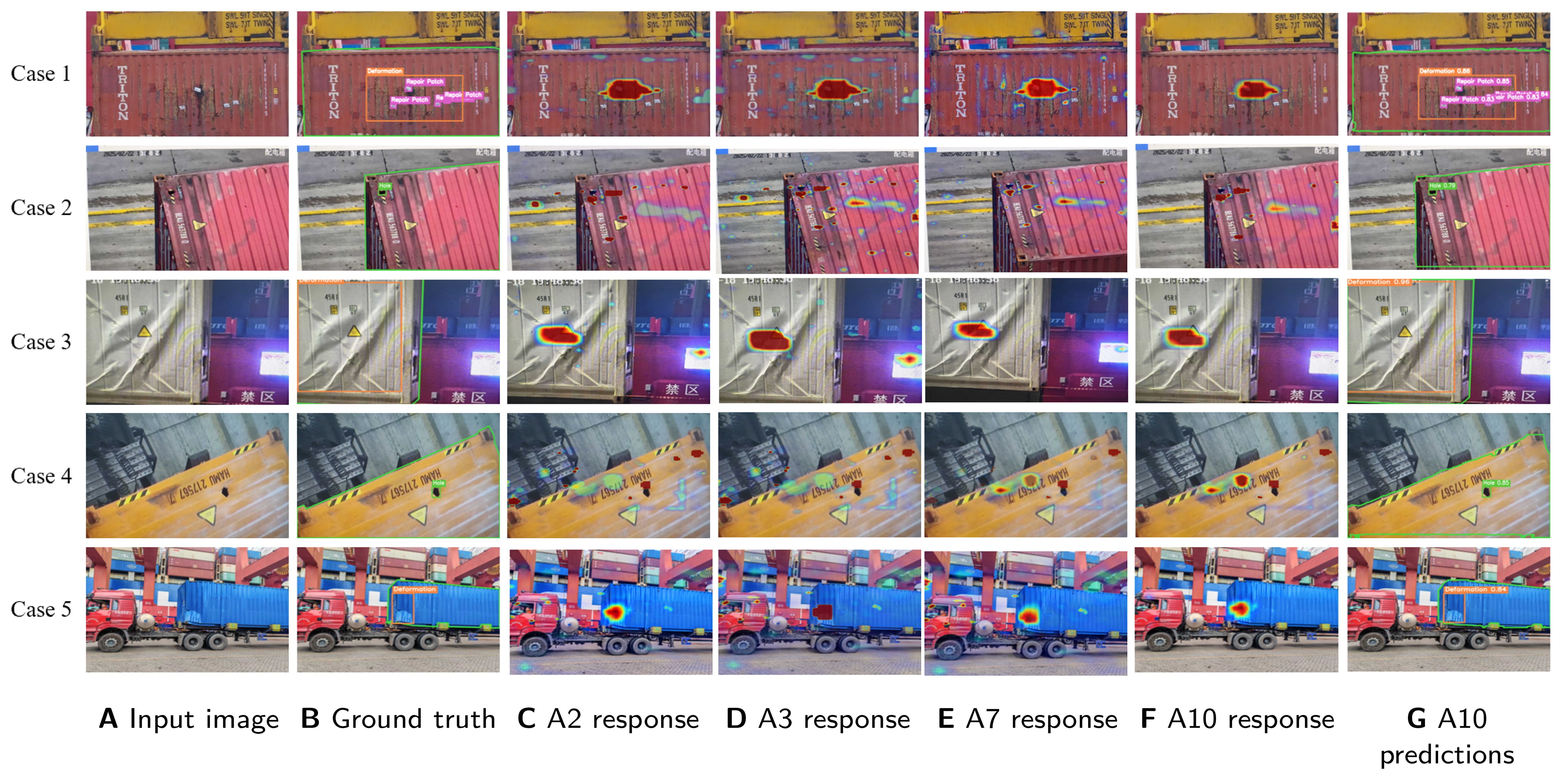
Figure 6. Detection-response heatmaps of the ablation configurations on five illustrative test images. Columns A and B show the input images and ground-truth annotations. Columns C-F show responses for A2 (detection and segmentation), A3 (A2 with STFF), A7 (A3 with bidirectional MG-CTI), and A10 (A7 with CTC and EAMR), respectively. Column G shows the final predictions of the complete CSG-YOLO model (A10). The cases illustrate individual response patterns rather than a statistically representative sample of the test set. STFF: Scale-tuned feature fusion; MG-CTI: mask-guided cross-task interaction; CTC: center-to-container consistency; EAMR: edge-aware mask refinement.
The five cases were selected to show a routine handling scene, road cracks and stains in an overhead view, a nearby light source, hole-like truck-frame structures, and a cluttered frontal view, respectively. In Case 1, all four configurations retain a main response around the damaged container region, while the spread of surrounding responses differs. In Case 2, responses to road and container-surface patterns vary across configurations, and some non-defect hotspots remain in A10. In Case 3, the nearby light source is prominent in the A2 and A3 maps but less prominent in the A7 and A10 maps, while the response on the deformed container surface is retained. Case 4 shows residual responses around truck-frame structures even in the complete model, illustrating that spatial guidance is a soft feature modulation rather than a hard exclusion of background. In Case 5, the main response lies on the deformed container, with additional responses around the truck and surrounding structures varying across the four maps.
These comparisons visualize how the response distribution changes with feature fusion, task interaction, and the additional training constraints. The A7-A10 comparison reflects the combined effect of CTC and EAMR; their individual contributions are evaluated by the A7-A8 and A9-A10 comparisons for EAMR and the A7-A9 and A8-A10 comparisons for CTC in Table 5. Heatmap colors are interpreted qualitatively rather than as calibrated cross-model scores or final detections. Overall detection and false-alarm performance is assessed on the complete 800-image test set using the AP, OMD, FPPI, and ODR results, while Boundary IoU supplies the boundary-sensitive evaluation of EAMR.
3.8. Qualitative comparison
As a visual complement to the quantitative results, Figure 7 compares CSG-YOLO with D-FINE, YOLO26, and RF-DETR on five illustrative test images. The selection is intended to show detection behavior in a routine scene and under four visually identifiable conditions: complex surface textures, mild non-defective contamination, a small hole, and image blur. These cases support inspection of specific detection outcomes and do not constitute a statistically representative sample of the test-set distribution. These competitors cover recent YOLO-series and transformer-based detection paradigms and are all included in the quantitative comparisons of Tables 1 and 2. The displayed predictions follow the common evaluation settings described in Section 3.3, including the 640 × 640 input resolution and confidence threshold of 0.25. Green polygonal contours delineate container-surface regions; the contour in the ground-truth column is the reference annotation, whereas that in the CSG-YOLO column is the predicted surface boundary.
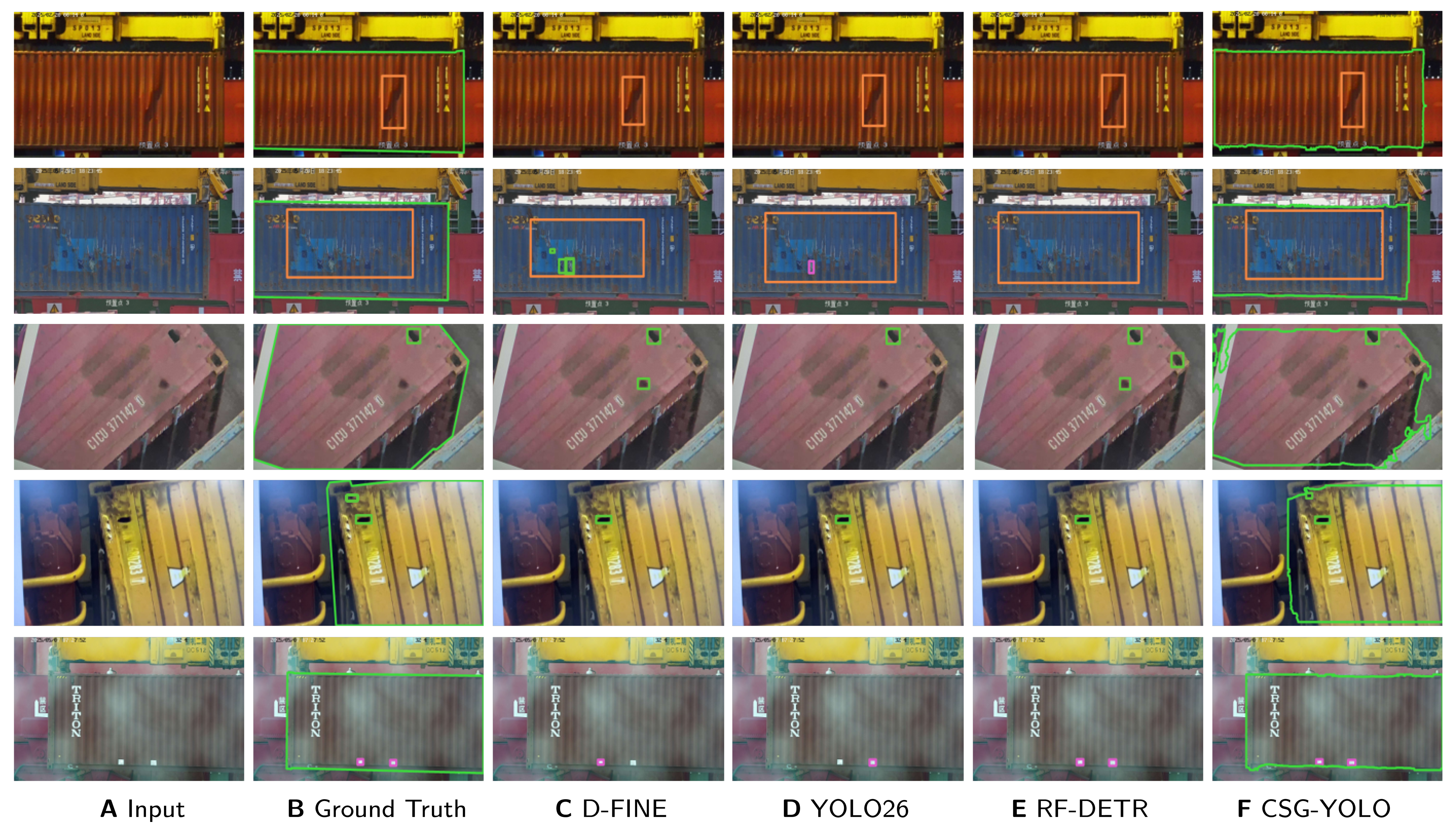
Figure 7. Qualitative comparison on illustrative inspection cases. Columns A-F show the input image, ground truth, D-FINE[33], YOLO26[30], RF-DETR[35], and CSG-YOLO, respectively. All displayed predictions were generated in this study. The references identify the compared detector architectures, rather than the sources of the images or prediction results. The displayed cases illustrate specific detection behaviors and do not establish performance across the test-set distribution.
In the routine scene of the first row, all four detectors correctly localize the defect. The second row contains complex container-surface textures: D-FINE and YOLO26 produce texture-induced false detections, whereas RF-DETR and CSG-YOLO avoid these distractors. In the third row, the container surface contains only a small area of mild, non-defective contamination. Among the competing detectors, D-FINE and RF-DETR confuse this ordinary stain with a hole, while YOLO26 and CSG-YOLO avoid this category confusion. The fourth row presents a genuinely damaged small hole; all three competing methods miss this compact target, whereas CSG-YOLO detects it correctly. In the blurred scene of the fifth row, D-FINE and YOLO26 miss the layered repair-patch instances, while RF-DETR and CSG-YOLO retain the corresponding detections. In these particular images, CSG-YOLO avoids the illustrated texture- and stain-induced false detections and retains the displayed small-hole and blurred repair-patch detections, while also estimating the container-surface boundary. These observations are limited to the displayed cases and do not establish robustness under every instance of these conditions, their occurrence rates, or average superiority over the competing methods. Overall performance is assessed using AP, OMD, FPPI, and ODR on the complete 800-image test set under the common evaluation protocol, as reported in Tables 1 and 2; the qualitative examples serve only to illustrate individual model behaviors.
3.8.1. Failure cases
Figure 8 presents four illustrative failure cases of CSG-YOLO in a 2 × 2 layout, with each case showing ground-truth annotations, model predictions, and an enlarged region. In the upper-left case, the missed hole beside the container identification number occupies approximately 11 × 13 pixels at the 640 × 640 input resolution; its fine spatial cues may be weakened by subsequent feature downsampling. In the lower-left case, the hole partially occluded by a lashing strap is detected with confidence 0.28, slightly above the evaluation threshold of 0.25, while strongly reflective folds produce an additional false hole prediction with confidence 0.71. Thus, this case combines a low-confidence true detection with a reflection-induced false positive. In the overhead roof view of the upper-right case, worn and deformed locking hardware is mistaken for a defect hole, and the predicted surface mask extends into the background. In the lower-right case, a hole spans the junction between the container panel and lower beam, but the predicted box covers only its lower part, giving an IoU of 0.26 and failing the IoU ≥ 0.50 localization criterion.
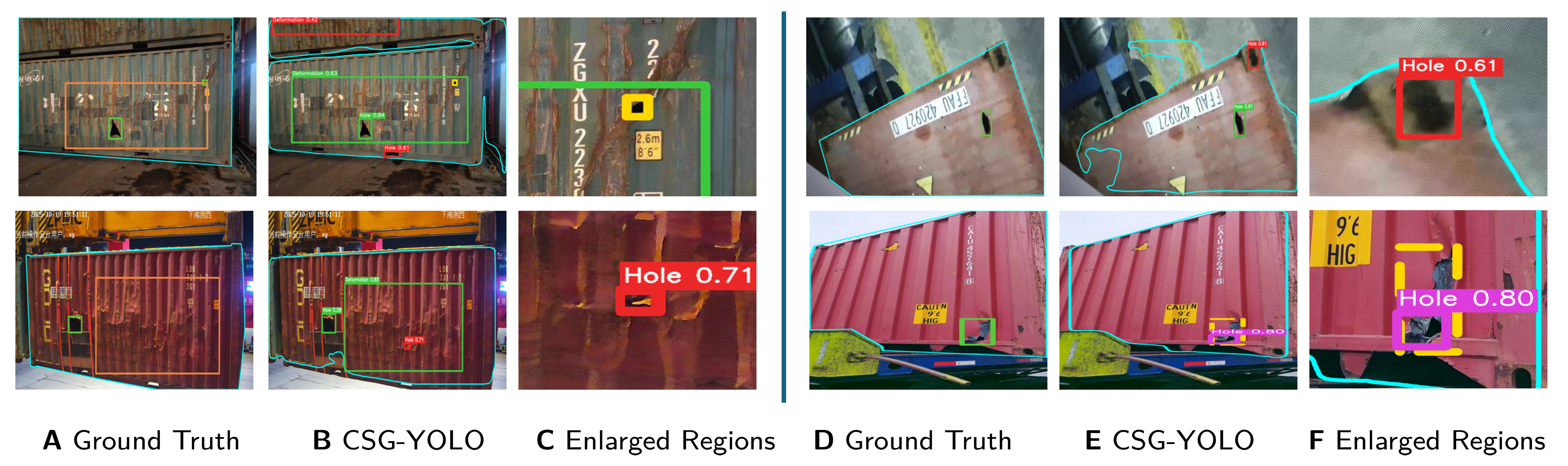
Figure 8. Four illustrative failure cases of CSG-YOLO in a 2 × 2 layout. Within each half of the figure, columns A-C (left) and D-F (right) show ground-truth annotations, model predictions, and enlarged regions, respectively. Surface contours in columns A and D denote ground-truth container-surface boundaries, whereas those in columns B and E denote predicted boundaries. The upper-left case shows a missed tiny hole; the lower-left case shows a reflection-induced false positive alongside an occluded true hole; the upper-right case shows confusion with locking hardware and mask spillover; and the lower-right case shows incomplete localization near the panel–beam boundary.
These examples illustrate limitations associated with tiny-defect resolution, defect-like reflective or structural patterns, and unreliable surface priors in unusual views or near container boundaries.
3.9. Limitations and cross-port generalization
The present evaluation is restricted to a single dataset acquired using quay-crane cameras at Qianwan Terminal, Port of Qingdao, and a fixed training/test split. Although the subsets are independent at the physical-container level, both originate from the same terminal and acquisition setting. The reported results therefore characterize performance on held-out containers within this source environment, rather than establish generalization to unseen ports. Repeating training with different random seeds measures training variability under this split and does not provide evidence of robustness to domain shift.
Changes in port infrastructure and background clutter, container types and surface appearance, camera sensors and optics, illumination and weather, and inspection geometry, viewing distance, and camera angle may alter both defect appearance and the distribution of valid container surfaces. Such shifts may affect defect localization and classification as well as surface-mask estimation. Since detection uses the learned surface prior through MG-CTI, degradation of that prior in an unfamiliar acquisition setting may also weaken its guidance. These effects have not been quantified by the current experiments, and the observed gains should not be assumed to transfer unchanged across environments.
No compatible external container-defect dataset with both defect bounding boxes and container-surface masks under a matching annotation protocol was available to the authors for this study. Consequently, no external cross-port evaluation is reported. Future work will collect and consistently annotate data from additional ports and camera systems, evaluate independent target environments under varied container, illumination, weather, and viewing conditions, and assess any adaptation or recalibration required before deployment.
The learned surface representation is an auxiliary cue rather than a guaranteed valid detection domain. As the failure cases illustrate, unusual views and boundary regions can produce mask spillover or incomplete defect localization. The directional ablations show that improvements in auxiliary mask metrics do not uniformly translate into gains in all detection metrics.
The engineering metrics also have a limited interpretation: OMD and FPPI are class-agnostic and evaluated at one confidence threshold, while ODR checks box centers rather than full-box coverage. Three training runs quantify observed variability under the fixed split but do not establish statistical significance for small gains. Confidentiality restrictions on data and implementation limit independent reproduction.
Runtime measurements are limited to the experimental RTX 4090 D platform and do not establish performance on low-power edge devices. Evaluation on such devices remains future work, including latency, memory use, power consumption, and detection accuracy after model conversion.
4. CONCLUSIONS
This article presented a container-surface-guided dual-task framework for defect detection in complex port scenes. CSG-YOLO jointly models defect detection and surface segmentation, uses STFF to enhance multi-scale shared features, and employs MG-CTI to exchange complementary cues between the task heads. Directional ablations associate S → D with improved false-positive and outside-ROI suppression and D → S with improved surface-mask overlap and strict-IoU localization; the bidirectional configuration has the highest mean AP and lowest mean OMD and ODR among the interaction variants. Across three independent training runs using randomly generated seeds, CSG-YOLO-N improves mean AP, AP50, and AP75 over YOLOv12-N by 2.4, 3.2, and 4.1 points, respectively, while reducing mean OMD, FPPI, and ODR. The current evidence is confined to a single-terminal dataset, and cross-port or cross-camera generalization has not been demonstrated. Future work will prioritize external validation under domain shift, alongside further optimization for real-time deployment on edge inspection devices.
DECLARATIONS
Authors’ contributions
Made substantial contributions to conception and design of the study, performed data analysis and interpretation, and wrote the manuscript: Zhen, M.
Provided technical guidance and reviewed the manuscript: Zhao, J.; Jia, N.; Zhao, W.
Reviewed the manuscript: Zhen, M.
Availability of data and materials
This study uses a private dataset of 4,000 still images acquired by quay-crane cameras at Qianwan Terminal, Port of Qingdao, China. The authors obtained permission to use the images for research and prepared the defect bounding-box annotations and container-surface masks, as described in Section 3.1. The images and annotations are not publicly available because of confidentiality obligations under the applicable data-use and port-related agreements. The associated model source code, configuration files, trained weights, and evaluation scripts are also not publicly released under these restrictions. The manuscript describes the model architecture, key hyperparameters, training protocol, and evaluation procedures to support methodological transparency.
AI and AI-assisted tools statement
During the preparation of this manuscript, ChatGPT powered by GPT-5.6 Sol (OpenAI, released 2026-07-09) was used solely for language editing. The tool did not influence the study design, data collection, analysis, interpretation, or the scientific content of the work. All authors take full responsibility for the accuracy, integrity, and final content of the manuscript.
Financial support and sponsorship
This work was supported in part by the National Natural Science Foundation of China (Grant 62403361).
Conflicts of interest
All authors declared that there are no conflicts of interest.
Ethical approval and consent to participate
Not applicable.
Consent for publication
Not applicable.
Copyright
© The Author(s) 2026.
REFERENCES
1. Lusiani, M.; Zulkarnain; Komarudin. Object detection in container terminals based on deep learning approach: a systematic literature review. In 2024 IEEE International Conference on Industrial Engineering and Engineering Management (IEEM), Bangkok, Thailand. Dec 15-18, 2024. IEEE; 2024. pp. 0560-5.
2. Liu, Y.; Chen, H. A lightweight container detection network model based on YOLOv5s. In 2023 42nd Chinese Control Conference (CCC), Tianjin, China. Jul 24-26, 2023. IEEE; 2023. pp. 4267-72.
3. Pambudi, D. S.; Handayani, R.; Hidayah, L. Template matching algorithm for noise detection in cargo container. In 2018 Third International Conference on Informatics and Computing (ICIC), Palembang, Indonesia. Oct 17-18, 2018. IEEE; 2018. p. 1-9.
4. İmamoğlu, Z. E.; Tuğlular, T.; Baştanlar, Y. Container damage detection and classification using container images. In 2020 28th Signal Processing and Communications Applications Conference (SIU), Gaziantep, Turkey. Oct 05-07, 2020. IEEE; 2020. p. 1-4.
5. Huang, X. R.; Huang, G. Z.; Kuo, S. Y.; Chen, L. B. A vision transformer model-based shipping container damage inspection scheme. In 2024 International Conference on Consumer Electronics - Taiwan (ICCE-Taiwan), Taichung, Taiwan. Jul 09-11, 2024. IEEE; 2024. pp. 817-18.
6. Kuo, S. Y.; Lin, P. C.; Huang, X. R.; Huang, G. Z.; Chen, L. B. Cad-Transformer: a CNN–transformer hybrid framework for automatic appearance defect classification of shipping containers. IEEE. Trans. Instrum. Meas. 2025, 74, 1-21.
7. Huang, Y.; Chen, H.; Zheng, Z.; Jia, Y.; Chen, G. Attention-enhanced YOLO-based framework for container damage detection in port environments. In 2026 5th International Symposium on Computer Applications and Information Technology (ISCAIT), Dongguan, China. Jan 23-25, 2026. IEEE; 2026. pp. 493-7.
8. Zhao, Z. Research on port container damage detection algorithm based on C2PSA-improved YOLOv11. In 2026 5th International Symposium on Computer Applications and Information Technology (ISCAIT), Dongguan, China. Jan 23-25, 2026. IEEE; 2026; pp. 79-83.
9. Zheng, Y.; Shi, X.; Zhou, Y.; Hu, K.; Li, W. Container damage detection method based on improved YOLOv8. In 2025 6th International Conference on Big Data, Artificial Intelligence and Internet of Things Engineering (ICBAIE), Shanghai, China. Oct 17-19, 2025. IEEE; 2025. pp. 220-3.
10. Bahrami, Z.; Zhang, R.; Rayhana, R.; Wang, T.; Liu, Z. Optimized deep neural network architectures with anchor box optimization for shipping container corrosion inspection. In 2020 IEEE Symposium Series on Computational Intelligence (SSCI), Canberra, Australia. Dec 01-04, 2020. IEEE; 2020. pp. 1328-33.
11. Nguyen Thi Phuong, T.; Cho, G. S.; Chatterjee, I. Automating container damage detection with the YOLO-NAS deep learning model. Sci. Prog. 2025, 108, 00368504251314084.
12. Zhang, L. Container damage detection based on self contrastive learning and deep convolutional neural networks. In 2025 5th International Conference on Electronic Communication, Computer Science and Technology (ECCST), Qinhuangdao, China. Dec 26-28, 2025. IEEE; 2025. pp. 221-5.
13. Vasileiadis, S.; Aslam, S.; Orphanides, K.; et al. Real-time container tracking and damage detection at seaports using deep learning. In 20th Conference on Computer Science and Intelligence Systems (FedCSIS), Kraków, Poland. Sep 14-17, 2025. IEEE; 2025. pp. 277-85.
14. Rahman, A.; Khan, M. S. H.; Tazwar, M.; Rahat, M. T.; Nur, K. AutoContDamage: automated container damage detection in ports using RF-DETR model for enhanced operational efficiency. In 2025 28th International Conference on Computer and Information Technology (ICCIT), Cox’s Bazar, Bangladesh. Dec 19-21, 2025. IEEE; 2025. pp. 2986-91.
15. Li, X.; Huang, X.; Liu, Q. Container damage identification based on RP-FCN. In 2020 39th Chinese Control Conference (CCC), Shenyang, China. Jul 27-29, 2020. IEEE; 2020. pp. 7031-4.
16. Wang, H.; Liu, Q.; Zhang, G. Container damage detection algorithm based on fast-solo. In Proceedings of 2022 Chinese Intelligent Systems Conference. Jia, Y.; Zhang, W.; Fu, Y.; Zhao, S.; Eds; Singapore: Springer Nature Singapore; 2022. pp. 119-31.
17. Su, W.; Yu, N. An end-to-end detection and segmentation model for container surface damage based on YOLOv11. In 2025 5th International Conference on Electronic Information Engineering and Computer Communication (EIECC), Wuhan, China. Dec 26-28, 2025. IEEE; 2025. pp. 928-32.
18. Ornelas, D.; Canedo, D.; Neves, A. J. R. Semantic segmentation of corrosion in cargo containers using deep learning. Sustainability 2025, 17, 6480.
19. Liu, Z.; Zhao, W.; Jia, N.; Liu, X.; Yang, J. SANet: scale-adaptive network for lightweight salient object detection. Intell. Robot. 2024, 4, 503-23.
20. Božič, J.; Tabernik, D.; Skočaj, D. Mixed supervision for surface-defect detection: from weakly to fully supervised learning. Comput. Ind. 2021, 129, 103459.
21. He, K.; Gkioxari, G.; Dollár, P.; Girshick, R. Mask R-CNN. In 2017 IEEE International Conference on Computer Vision (ICCV). Venice, Italy. Oct 22-29, 2017. IEEE; 2017. pp. 2980-8.
22. Xu, D.; Ouyang, W.; Wang, X.; Sebe, N. PAD-Net: multi-tasks guided prediction-and-distillation network for simultaneous depth estimation and scene parsing. In 2018 IEEE/CVF Conference on Computer Vision and Pattern Recognition (CVPR), Salt Lake City, USA. Jun 18-23, 2018. IEEE; 2018. pp. 675-84.
23. Tian, Y.; Ye, Q.; Doermann, D. YOLOv12: attention-centric real-time object detectors. In Proceedings of the 39th International Conference on Neural Information Processing Systems, San Diego, USA and Mexico City, Mexico. Curran Associates Inc.; 2025. pp. 78433-57.
24. Woo, S.; Park, J.; Lee, J. Y.; Kweon, I. S. CBAM: convolutional block attention module. In Computer Vision - ECCV 2018. Cham: Springer International Publishing; Ferrari, V.; Hebert, M.; Sminchisescu, C.; Weiss, Y.; Eds; Springer, Cham; 2018. pp. 3-19.
25. COCO API: Python Detection Evaluation (cocoeval.py). https://github.com/cocodataset/cocoapi/blob/master/PythonAPI/pycocotools/cocoeval.py. (accessed 2026-10-23).
26. Cheng, B.; Girshick, R.; Dollár, P.; Berg, A. C.; Kirillov, A. Boundary IoU: improving object-centric image segmentation evaluation. In 2021 IEEE/CVF Conference on Computer Vision and Pattern Recognition (CVPR), Nashville, USA. Jun 20-25, 2021. IEEE; 2021; pp. 15329-37.
27. Wang, A.; Chen, H.; Liu, L.; et al. YOLOv10: real-time end-to-end object detection. In Proceedings of the 38th International Conference on Neural Information Processing Systems, Vancouver, Canada. Curran Associates Inc.; 2024. pp. 107984-8011.
28. Jocher, G.; Qiu, J. Ultralytics YOLO11. Version 11.0.0; 2024. https://github.com/ultralytics/ultralytics. (accessed 2026-10-23).
29. Lei, M.; Li, S.; Wu, Y.; et al. YOLOv13: real-time object detection with hypergraph-enhanced adaptive visual perception. arXiv 2025, arXiv:2506.17733. Available online: https://doi.org/10.48550/arXiv.2506.17733. (accessed 2026-10-23).
30. Jocher, G.; Qiu, J.; Liu, M.; et al. Ultralytics YOLO26: unified real-time end-to-end vision models. arXiv 2026, arXiv:2606.03748. Available online: https://doi.org/10.48550/arXiv.2606.03748. (accessed 2026-10-23).
31. Zhao, Y.; Lv, W.; Xu, S.; et al. DETRs beat YOLOs on real-time object detection. In 2024 IEEE/CVF Conference on Computer Vision and Pattern Recognition (CVPR), Seattle, USA. Jun 16-22, 2024. IEEE; 2024; pp. 16965-74.
32. Lv, W.; Zhao, Y.; Chang, Q.; Huang, K.; Wang, G.; Liu, Y. RT-DETRv2: improved baseline with bag-of-freebies for real-time detection transformer. arXiv 2024, arXiv:2407.17140. Available online: https://doi.org/10.48550/arXiv.2407.17140. (accessed 2026-10-23).
33. Peng, Y.; Li, H.; Wu, P.; Zhang, Y.; Sun, X.; Wu, F. D-FINE: redefine regression task of DETRs as fine-grained distribution refinement. In International Conference on Learning Representations; 2025. pp. 44015-31. https://proceedings.iclr.cc/paper_files/paper/2025/file/6cf58a87e3097e7d1f9be3e8693a93de-Paper-Conference.pdf. (accessed 2026-10-23).
34. Huang, S.; Lu, Z.; Cun, X.; Yu, Y.; Zhou, X.; Shen, X. DEIM: DETR with improved matching for fast convergence. In 2025 IEEE/CVF Conference on Computer Vision and Pattern Recognition (CVPR), Nashville, USA. Jun 10-17, 2025. IEEE; 2025. pp. 15162-71.
35. Robinson, I.; Robicheaux, P.; Popov, M.; Ramanan, D.; Peri, N. RF-DETR: neural architecture search for real-time detection trans-formers. In International Conference on Learning Representations; 2026. https://proceedings.iclr.cc/paper_files/paper/2026/file/5bed8703db85ab27dc32f6a42f8fbdb6-Paper-Conference.pdf. (accessed 2026-10-23).
Cite This Article
 Open Access
How to Cite
Zhen, M.; Zhao, W.; Zhao, J.; Jia, N. Container-surface-guided dual-task learning for defect detection in complex port scenes. Intell. Robot. 2026, 6(4), 811-42. https://dx.doi.org/10.20517/ir.2026.36
Download Citation
If you have the appropriate software installed, you can download article citation data to the citation manager of your choice. Simply select your manager software from the list below and click on download.
Export Citation File
Type of Import
Tips on Downloading Citation
Citation Manager File Format
Type of Import
Direct Import: When the Direct Import option is selected (the default state), a dialogue box will give you the option to Save or Open the downloaded citation data. Choosing Open will either launch your citation manager or give you a choice of applications with which to use the metadata. The Save option saves the file locally for later use.
Indirect Import: When the Indirect Import option is selected, the metadata is displayed and may be copied and pasted as needed.
About This Article
Copyright

Data & Comments
Data
0










Comments
Comments must be written in English. Spam, offensive content, impersonation, and private information will not be permitted. If any comment is reported and identified as inappropriate content by OAE staff, the comment will be removed without notice. If you have any queries or need any help, please contact us at [email protected].