



ConCast: a CBAM-enhanced SimVP with temporal consistency regularization for precipitation nowcasting
 0
0 
Abstract
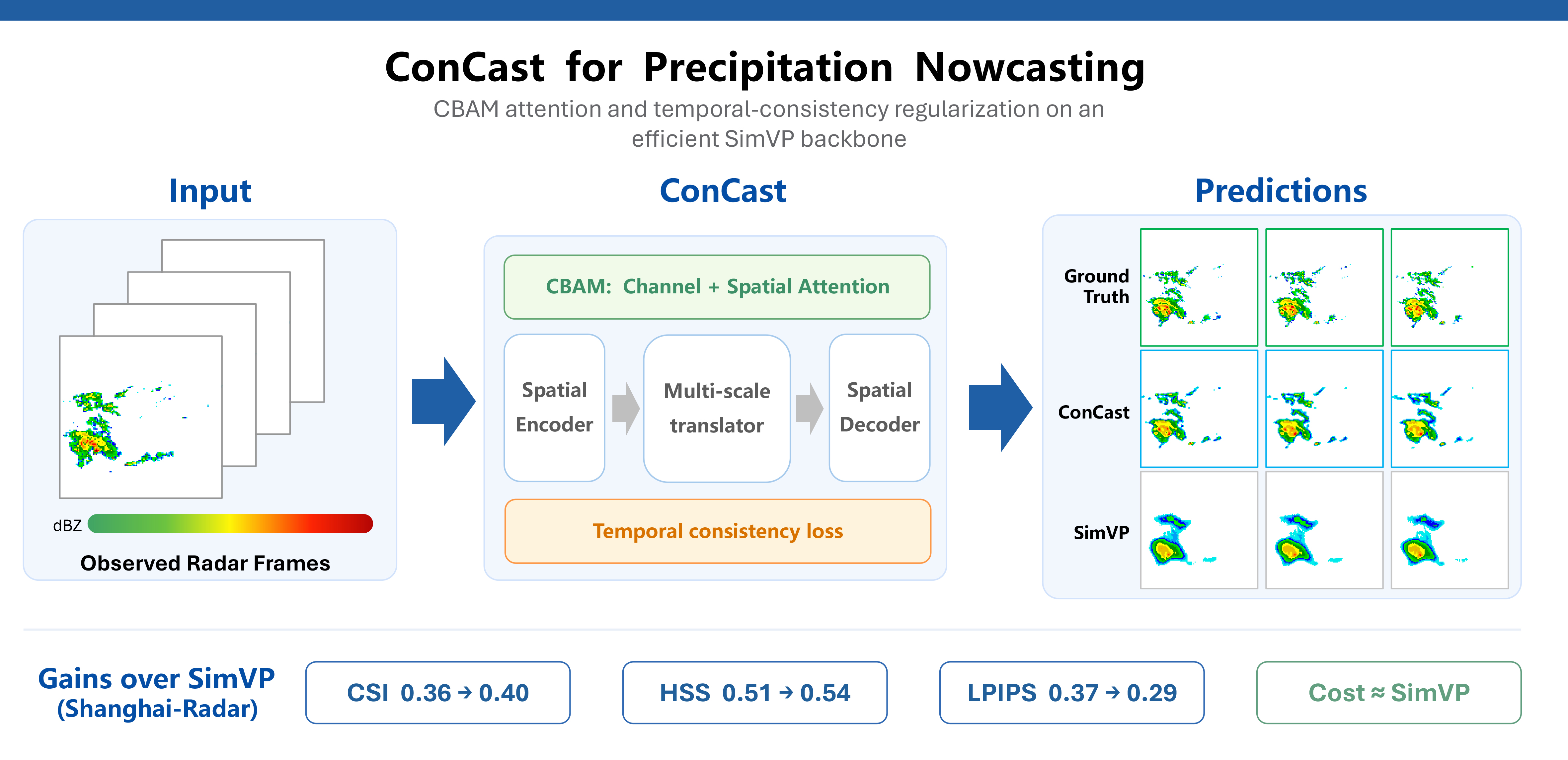
Precipitation nowcasting is essential for weather warning and rapid-response decision-making, yet existing deep spatiotemporal models often struggle to emphasize meteorologically salient echo structures and to keep their predictions coherent across future frames. We address these issues with ConCast, an enhanced SimVP for radar-based precipitation nowcasting that couples convolutional block attention module (CBAM) refinement with temporal consistency regularization (TCR). The CBAM stage strengthens channel-wise and spatial feature selection so that the network attends to informative precipitation patterns, whereas an auxiliary cosine consistency term constrains the relationship between successive predictions during training. On the Shanghai-Radar and SEVIR datasets, ConCast improves forecasting quality over representative baselines and produces sharper and temporally steadier echo fields. Ablation studies show that the two components act on different aspects of the problem, with attention sharpening spatial discrimination and the consistency term improving sequence coherence, and that their gains do not overlap. Because ConCast adds only marginal overhead to SimVP, attention refinement combined with TCR is a practical option for nowcasting.
Keywords
1. INTRODUCTION
Very short-term precipitation forecasting, commonly referred to as precipitation nowcasting, aims to predict the evolution of rainfall over the next few minutes to several hours. Reliable nowcasting is particularly important in densely populated regions, where sudden convective events can rapidly trigger traffic disruption, urban flooding, and operational risks in transportation and energy systems. Traditional numerical weather prediction (NWP)[1] provides physically grounded forecasts, while radar echo extrapolation methods, such as tracking radar echoes by correlation (TREC)[2] and optical-flow-based nowcasting[3], remain important tools for real-time operational forecasting. Seamless or blending systems further combine NWP guidance with extrapolation to exploit their complementary strengths across lead times[4]. In contrast, deep learning methods can learn precipitation dynamics directly from historical observations, enabling fast inference and flexible deployment.
Deep learning has made substantial progress in spatiotemporal sequence forecasting. Recurrent neural network (RNN)-based models, such as ConvLSTM[5], TrajGRU[6], PredRNN[7], PredRNN++[8], MIM[9], SwinLSTM[10], PhyDNet[11], and MAU[12], process images sequentially and preserve temporal continuity through hidden-state transitions. These models are effective for local motion modeling, but their recurrent nature can weaken long-range dependency learning and increase optimization difficulty over extended forecasting horizons. Related video prediction studies, including action-conditioned and stochastic formulations[13-16], likewise emphasize the importance of motion realism and multi-step stability.
More recent direct prediction architectures, such as SimVP[17], Tau[18], and Earthformer[19], jointly model multiple historical frames and directly decode future sequences. In the broader weather forecasting literature, large-context and foundation-style models such as MetNet[20], its 12-hour forecasting variant[21], FourCastNet[22], Pangu-Weather[23], GraphCast[24], and ClimaX[25] have further demonstrated the scalability of data-driven forecasting across longer horizons and larger spatial domains. Such models are computationally attractive and easier to parallelize, yet they may still produce overly smooth predictions or lose sharp local structures, particularly when the model fails to emphasize the most relevant echo regions. SimVP is selected as the baseline in this work because of its simple encoder-mid-decoder design, strong efficiency, and competitive performance without relying on recurrent connections or transformer self-attention.
Generative and probabilistic forecasting strategies have also been introduced to improve the realism of the output. Methods such as CasCast[26], SV2P[27], STRPM[28], DGMR[29], NowcastNet[30], DiffCast[31], and ExtremeCast[32] improve sharpness or uncertainty modeling by redesigning architectures and training objectives. Nevertheless, two challenges remain central in radar-based nowcasting: identifying the most informative regions in cluttered echo scenes and maintaining stable temporal transitions across successive predicted frames.
To address these challenges, we propose ConCast, an enhanced SimVP model for precipitation nowcasting with two complementary components:
● Convolutional block attention module (CBAM): CBAM[33] guides the model to focus on informative channel-wise and spatial features while suppressing irrelevant information.
● Temporal consistency regularization (TCR): A cosine consistency loss is applied across successive predictions to provide additional temporal regularization during training.
ConCast therefore aims to sharpen spatial discrimination and prediction coherence simultaneously while maintaining the low computational footprint of SimVP. The remainder of this paper reviews related work, describes the proposed method, reports the experimental results, and discusses their implications.
The main contributions of this work are summarized as follows:
● We propose ConCast, a lightweight precipitation nowcasting framework that enhances SimVP with CBAM-based feature refinement and TCR.
● We validate the proposed framework on two heterogeneous benchmarks, Shanghai-Radar and SEVIR, covering both regional radar forecasting and broader cross-scene evaluation.
● We provide quantitative and ablation evidence showing that the two components address different aspects of the task and together improve both forecasting quality and temporal consistency.
2. RELATED WORK
2.1. Operational and learning-based precipitation nowcasting
Precipitation nowcasting has attracted considerable attention for its role in real-time weather prediction. Operational systems have traditionally relied on two major sources of guidance. NWP models provide physically grounded atmospheric evolution but can be less responsive at very short lead times because of initialization, spin-up, and computational constraints[1]. Radar echo extrapolation methods, including TREC-based motion estimation[2] and enhanced optical-flow techniques[3], directly infer echo displacement from recent observations and are therefore widely used for immediate forecasts. In practice, seamless nowcasting systems often blend extrapolation with NWP so that observation-driven forecasts dominate early lead times and model guidance contributes increasingly at longer lead times[4].
Learning-based methods offer an alternative by training neural models to infer precipitation evolution from historical radar sequences. In recent years, data-driven nowcasting has evolved from early sequence modeling approaches toward more expressive architectures that aim to better capture precipitation motion, local structure, and uncertainty.
Existing nowcasting models mainly fall into three categories. Recurrent architectures, such as ConvLSTM[5], TrajGRU[6], PredRNN[7], PredRNN++[8], and MIM[9], model temporal evolution through hidden-state transitions and are effective for motion-aware prediction. Encoder-decoder approaches, including U-Net[34], RainNet[35], and related radar forecasting models[36], preserve spatial detail through multi-scale feature extraction and skip connections. More recent large-context and generative methods, such as MetNet[20], DGMR[29], NowcastNet[30], and DiffCast[31], further improve realism and forecasting quality by enlarging the receptive context or modeling uncertainty explicitly.
Despite this progress, accurately identifying salient echo regions and maintaining coherent multi-frame evolution remain challenging, especially for efficient radar-based nowcasting systems. These issues are particularly relevant when a model must preserve sharp local precipitation structures without sacrificing temporal stability across future predictions.
2.2. Attention mechanisms in weather prediction
Attention mechanisms have become an important tool for improving spatiotemporal prediction models by emphasizing informative regions and suppressing irrelevant responses. In precipitation nowcasting, this capability is particularly valuable because key echo structures often occupy only a limited portion of the scene, while surrounding areas may contain clutter or weak background patterns. Attention-based designs have been explored in both recurrent and non-recurrent forecasting models. For example, SwinLSTM[10] incorporates transformer-style attention into recurrent prediction, Tau[18] introduces temporal attention for efficient spatiotemporal predictive learning, and Earthformer[19] further demonstrates the effectiveness of space-time attention mechanisms in Earth system forecasting.
Beyond global or transformer-style attention, lightweight plug-in modules have also been widely studied for efficient feature refinement. CBAM[33] sequentially applies channel attention and spatial attention, while ECA-Net[37] shows that efficient channel attention alone can provide meaningful gains with minimal additional complexity. Compared with heavier attention mechanisms, such modules are attractive for radar nowcasting because they can enhance localized precipitation features, storm boundaries, and high-value echo regions without substantially increasing computation.
2.3. Temporal regularization for forecasting
Similarity-based objectives from representation learning encode structure by preserving similarity among related samples rather than relying solely on reconstruction. In time-series settings, Zhang et al.[38] examined what makes such objectives effective for forecasting, and SimTS[39] showed that simple similarity-based objectives improve forecasting-oriented sequence representations. These studies indicate that similarity constraints can help sequential models learn smoother and more discriminative temporal dynamics.
Temporal consistency has also been used as an explicit regularizer in video and sequence modeling. Lai et al.[40] enforce frame-to-frame consistency to stabilize per-frame processed video; temporal cycle-consistency learning[41] aligns embeddings across time through a differentiable consistency objective, and TCR has been applied to improve stability in domain-adaptive video segmentation[42]. A common theme across these works is that constraining the relationship between neighboring frames encourages temporally coherent outputs, which is particularly relevant for radar echo forecasting, where small inconsistencies between adjacent predictions may accumulate and lead to unrealistic precipitation evolution.
3. METHOD
3.1. SimVP architecture
The proposed method is built upon SimVP, which learns spatial and temporal dependencies from sequential radar echo images. As shown in Figure 1, the model takes a sequence of historical radar frames as input and predicts multiple future precipitation frames. The framework contains three main components: an encoder for hierarchical spatial feature extraction, a spatiotemporal module for latent dynamics modeling, and a decoder for reconstructing the future sequence. CBAM is inserted into the feature transformation pipeline to refine informative channel-wise and spatial responses. During training, the predicted sequence is supervised by a pixel-wise reconstruction loss and an auxiliary temporal consistency loss between adjacent predictions.
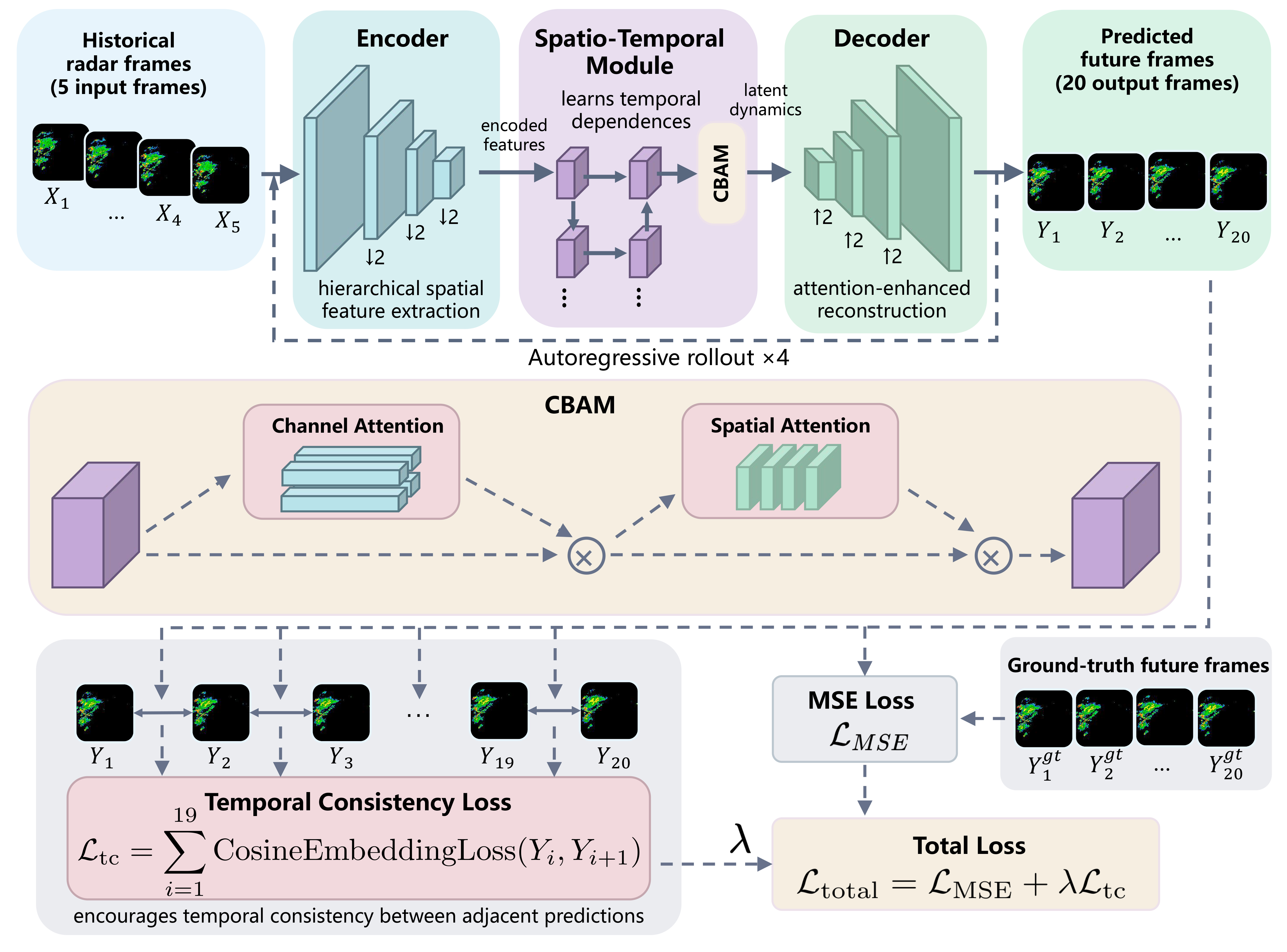
Figure 1. Overall framework of the proposed method. Historical radar frames are first encoded into hierarchical spatial features, then processed by a spatio-temporal module with CBAM refinement, and finally decoded into future precipitation frames. SimVP predicts five frames per forward pass, and four autoregressive rollouts generate the complete 20-frame forecast. Only representative frames are shown for clarity. During training, the predictions are jointly supervised by the MSE loss and the temporal consistency loss. CBAM: Convolutional block attention module; MSE: mean squared error.
More specifically, let the input radar sequence be
Formally, after reshaping
where
After spatial encoding, the latent tensor is rearranged back to the sequence form and passed to a middle spatiotemporal translator. The latent sequence is reshaped from
Let
For each multi-scale translation block, the hidden feature is computed as
where
where
Finally, the decoder mirrors the encoder by using the reversed stride schedule to progressively recover spatial resolution. The first-stage encoder feature is preserved as a shallow skip connection and is concatenated with the last decoder feature before the final reconstruction block. A
The decoder output is therefore obtained as
where
3.2. Encoder-decoder with CBAM
The encoder and decoder follow the general structure of an encoder-decoder network, with CBAM embedded to enhance attention to informative features. The encoder gradually downsamples the input sequence and extracts hierarchical representations, while the decoder upsamples the encoded features to generate future radar frames. This design preserves the computational simplicity of SimVP while strengthening the network's sensitivity to salient echo intensity patterns, storm boundaries, and localized precipitation cores.
The encoder uses repeated convolutional blocks, where stride-1 layers preserve the current spatial resolution, and stride-2 layers perform downsampling. The decoder follows the reverse process with upsampling blocks to progressively restore the original resolution. This alternating downsampling and upsampling strategy reduces computation while retaining a direct shallow skip path from the first encoder stage to the final reconstruction stage. Such a design helps recover fine precipitation structures that might otherwise be lost in the latent transformation process.
CBAM is applied sequentially with a channel-attention stage followed by a spatial-attention stage. Given an input feature map
where
For channel attention, global average pooling and global max pooling are first applied to
where
For spatial attention, channel-wise average pooling and max-pooling are computed on the channel-refined feature
where
3.3. TCR
To provide additional temporal regularization during training, a cosine consistency loss is applied across multiple predicted frames. The loss is computed between adjacent outputs so that neighboring predictions remain close in representation space while the mean squared error (MSE) term still anchors each frame to the ground truth. This regularization is particularly useful for multi-step nowcasting, where small inconsistencies introduced in early predictions may accumulate and lead to unrealistic echo evolution later in the sequence.
The temporal consistency loss is defined as
where
where
3.4. Overall loss function
The overall training objective combines the MSE loss with the temporal consistency loss:
where
The reconstruction term preserves pixel-level fidelity to the target radar field, while the temporal consistency term regularizes the trajectory of the predicted sequence in feature space. As a result, the model is encouraged not only to minimize frame-wise errors, but also to generate temporally coherent future evolution.
4. EXPERIMENTS
4.1. Experimental settings
Following prior work, the continuous radar sequences are divided into multiple events. Each event contains 25 frames, and the first 5 frames are used to predict the subsequent 20 frames. For SEVIR, this setting corresponds to forecasting the next 100 min from the previous 25 min of observations because the temporal interval is 5 min per frame. For Shanghai-Radar, where the frame interval is 6 min, the same protocol corresponds to forecasting the next 120 min from the previous 30 min of observations. All frames are resized to
The model is implemented in PyTorch. All models are trained on a server equipped with an Intel(R) Xeon(R) Gold 6448H @ 2.40 GHz CPU, eight NVIDIA A40 GPUs, and 1 TB of RAM. We train each model for 200 epochs using the AdamW optimizer with an initial learning rate of
4.2. Evaluation metrics
The models are assessed using CSI, HSS, bias score (BS), LPIPS, SSIM, temporal gradient error (TGE), and MSE. For threshold-based metrics, TP, FP, TN, and FN are computed after binarizing the predicted and ground-truth radar fields with the same intensity threshold. For Shanghai-Radar, we use reflectivity thresholds of 20, 30, 35, and 40 dBZ, with 35 dBZ as the primary strong-convection threshold. For SEVIR, we follow common VIL evaluation practice and use thresholds of 16, 74, 133, 160, 181, and 219. Unless otherwise specified, the main categorical analysis reports the mean score across the corresponding threshold set. Among these metrics, the pooled CSI variants (CSI-POOL4 and CSI-POOL16) are additionally reported in the main quantitative comparison, whereas BS and TGE are used in the ablation analysis to examine forecast bias and temporal coherence, respectively.
where CSI is also known as the threat score (TS),
where BS measures whether a model over-forecasts or under-forecasts event frequency. A value closer to 1 indicates a better balance between predicted and observed events. CSI-POOL4 and CSI-POOL16 are pooled CSI variants computed after applying spatial max-pooling with kernel sizes 4 and 16, respectively. These pooled scores relax small spatial displacement errors and evaluate whether the predicted precipitation event occurs in the neighboring region.
where TGE directly measures whether the temporal change between adjacent predicted frames matches the observed temporal change. Lower TGE indicates better temporal coherence relative to the ground truth.
where
and
4.3. Datasets
4.3.1. Shanghai-Radar dataset
The Shanghai-Radar dataset[43] was collected from the dual-polarization weather monitoring radar located in Pudong, Shanghai. It contains continuous radar echo frames acquired between October 2015 and July 2018. Each frame covers approximately
4.3.2. SEVIR dataset
The SEVIR dataset[44] includes satellite imagery, NEXRAD radar mosaics, and lightning event data. In this work, we use the VIL modality for precipitation forecasting. The dataset contains more than 20, 000 severe weather events, each lasting 4 h and covering an area of
4.4. Quantitative results
The results on the Shanghai-Radar and SEVIR datasets are summarized in Tables 1 and 2. Across most evaluation metrics, the proposed model outperforms the baselines, indicating superior forecasting skill and greater structural fidelity.
Performance comparison of different methods on the Shanghai-Radar dataset
| Method | CSI | CSI-POOL4 | CSI-POOL16 | HSS | LPIPS | SSIM | MSE |
| Higher values are better for CSI, CSI-POOL4, CSI-POOL16, HSS, and SSIM. Lower values are better for LPIPS and MSE. Bold and underlined values indicate the best and second-best results for each metric, respectively. MSE: Mean squared error. | |||||||
| SimVP | 0.3614 | 0.3803 | 0.4257 | 0.3691 | 0.7477 | ||
| PhyDNet | 0.5054 | 32.9153 | |||||
| Tau | 0.3652 | 0.3679 | 0.4186 | 0.5004 | 0.3730 | 0.7593 | 31.2825 |
| MAU | 0.3582 | 0.3776 | 0.4485 | 0.4923 | 0.3483 | 0.7451 | 33.1546 |
| Earthformer | 0.2222 | 0.2089 | 0.2353 | 0.3198 | 0.3726 | 0.6928 | 35.8055 |
| PredRNN | 0.1993 | 0.2158 | 0.2686 | 0.2779 | 0.4280 | 0.6532 | 54.0558 |
| PredRNN++ | 0.1855 | 0.2198 | 0.3325 | 0.2983 | 0.3593 | 0.6792 | 57.6103 |
| Ours | 0.4038 | 0.4384 | 0.5207 | 0.5419 | 0.2893 | 0.7824 | 29.4490 |
Performance comparison of different methods on the SEVIR dataset
| Method | CSI | CSI-POOL4 | CSI-POOL16 | HSS | LPIPS | SSIM | MSE |
| Higher values are better for CSI, CSI-POOL4, CSI-POOL16, HSS, and SSIM. Lower values are better for LPIPS and MSE. Bold and underlined values indicate the best and second-best results for each metric, respectively. MSE: Mean squared error. | |||||||
| SimVP | 0.2644 | 0.3411 | 0.4032 | 0.6123 | 492.88 | ||
| PhyDNet | 0.2631 | 0.2706 | 0.3095 | 0.3388 | 0.3852 | 0.6122 | 457.98 |
| Tau | 0.2578 | 0.2651 | 0.3072 | 0.3322 | 0.4205 | 0.5095 | 472.98 |
| MAU | 0.2638 | 0.2736 | 0.3245 | 0.3402 | 0.3631 | 0.6244 | 461.52 |
| Earthformer | 0.1882 | 0.1982 | 0.2238 | 0.2341 | 0.3458 | 0.5076 | 555.36 |
| PredRNN | 0.1622 | 0.1724 | 0.2156 | 0.2092 | 0.4116 | 0.5535 | 739.14 |
| PredRNN++ | 0.2768 | 0.3258 | 0.3598 | ||||
| Ours | 0.2765 | 0.2961 | 0.3489 | 0.3622 | 0.6317 | 445.03 | |
On the Shanghai-Radar dataset, the proposed model achieves the best results on all reported metrics. Relative to the SimVP baseline, it raises CSI from 0.3614 to 0.4038 and HSS from 0.5083 to 0.5419, while lowering LPIPS from 0.3691 to 0.2893 and MSE from 29.6566 to 29.4490. The pooled scores improve in parallel (CSI-POOL4 from 0.3803 to 0.4384 and CSI-POOL16 from 0.4257 to 0.5207), and the gains over the strongest competing baselines on CSI and SSIM further indicate that the proposed design better preserves local echo structures and fine-grained precipitation patterns rather than simply smoothing the output.
On the SEVIR dataset, the proposed model again achieves the best performance on CSI, CSI-POOL4, CSI-POOL16, HSS, SSIM, and MSE, while obtaining the second-best LPIPS. It reaches a CSI of 0.2765 and an HSS of 0.3622, exceeding both the SimVP baseline (0.2644 and 0.3411) and the strongest competing baseline, PredRNN++ (0.2663 and 0.3430), and attains the lowest MSE of 445.03. Its LPIPS of 0.3494 trails only Earthformer (0.3458), whose categorical skill is far lower (CSI 0.1882), so the small LPIPS gap does not reflect better forecasting ability. Because SEVIR contains more diverse storm morphologies and broader scene variability than Shanghai-Radar, these results indicate that the proposed framework generalizes effectively beyond a single regional radar distribution.
4.5. Dataset characteristics
The representative examples in Figures 2 and 3 illustrate the different visual characteristics of the two datasets. The Shanghai-Radar samples exhibit relatively concentrated regional echo structures, whereas SEVIR contains more diverse large-scale storm morphologies. This contrast highlights the value of evaluating the model on both a regional radar dataset and a more heterogeneous benchmark.
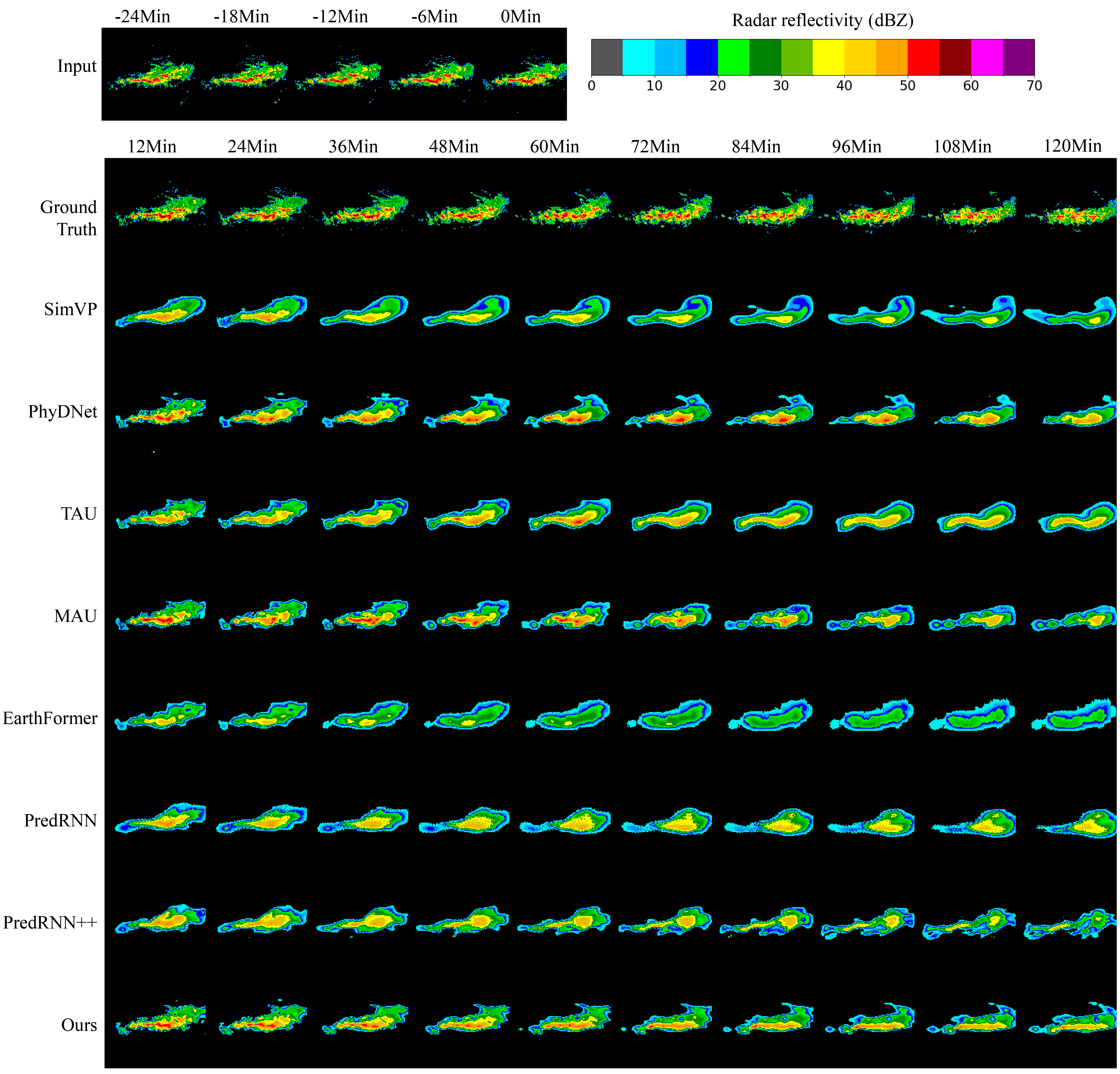
Figure 2. Visual examples from the Shanghai-Radar dataset. The samples exhibit relatively concentrated regional echo structures and localized precipitation evolution in the Shanghai area.
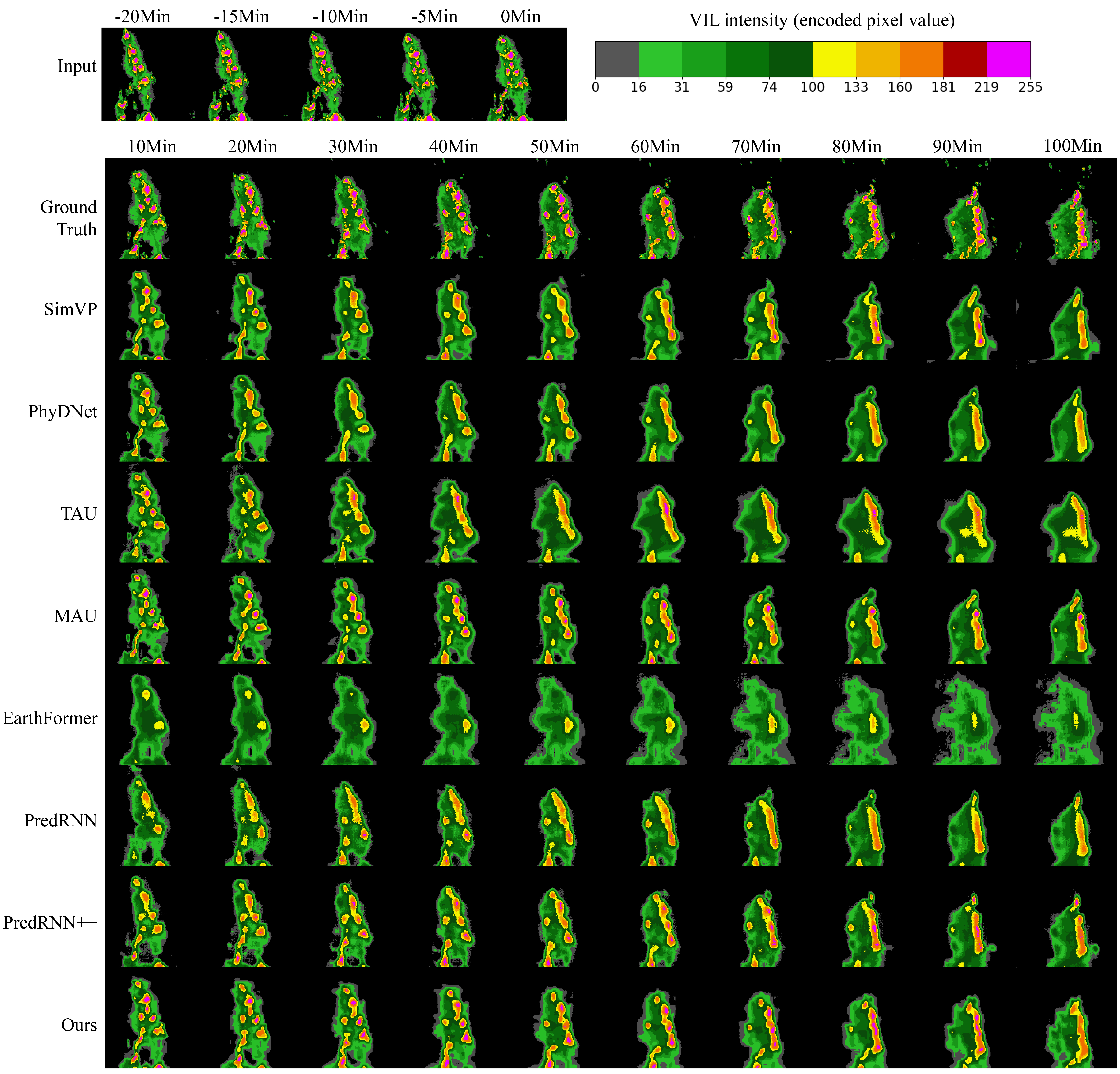
Figure 3. Visual examples from the SEVIR dataset using the VIL modality. The samples show more diverse storm structures and broader scene variability than Shanghai-Radar.
4.6. Ablation studies
To isolate the contribution of each component, we compare the SimVP baseline, SimVP with CBAM, SimVP with TCR, and the full ConCast model that combines both, as reported in Tables 3 and 4. This component-isolation protocol directly tests whether the attention module, the temporal regularization term, and their combination each contribute to final performance.
Component-isolation ablation on the Shanghai-Radar dataset
| Method | CSI | HSS | BS | TGE | LPIPS | SSIM | MSE |
| Bold values indicate the best result for each metric. BS: Bias score; TGE: temporal gradient error; MSE: mean squared error; CBAM: convolutional block attention module; TCR: temporal consistency regularization. | |||||||
| SimVP | 0.3614 | 0.5083 | 1.12 | 4.86 | 0.3691 | 0.7477 | 29.6566 |
| SimVP+CBAM | 0.3876 | 0.5298 | 1.06 | 4.68 | 0.3157 | 0.7758 | 29.5842 |
| SimVP+TCR | 0.3789 | 0.5236 | 1.04 | 4.31 | 0.3418 | 0.7645 | 29.5317 |
| Ours | 0.4038 | 0.5419 | 1.01 | 4.18 | 0.2893 | 0.7824 | 29.4490 |
Component-isolation ablation on the SEVIR dataset
| Method | CSI | HSS | BS | TGE | LPIPS | SSIM | MSE |
| Bold values indicate the best result for each metric. BS: Bias score; TGE: temporal gradient error; MSE: mean squared error; CBAM: convolutional block attention module; TCR: temporal consistency regularization. | |||||||
| SimVP | 0.2644 | 0.3411 | 1.15 | 18.92 | 0.4032 | 0.6123 | 492.88 |
| SimVP+CBAM | 0.2718 | 0.3547 | 1.09 | 18.21 | 0.3668 | 0.6264 | 462.37 |
| SimVP+TCR | 0.2696 | 0.3509 | 1.07 | 17.35 | 0.3821 | 0.6218 | 468.54 |
| Ours | 0.2765 | 0.3622 | 1.03 | 16.88 | 0.3494 | 0.6317 | 445.03 |
The component-isolation results in Tables 3 and 4 let us attribute the gains to each module separately. Relative to the SimVP baseline, adding CBAM yields a larger improvement in spatial skill and structural fidelity: on Shanghai-Radar, it lifts CSI from 0.3614 to 0.3876 and cuts LPIPS from 0.3691 to 0.3157, clearly exceeding the CSI of 0.3789 obtained by adding TCR alone. Adding TCR instead yields a pronounced reduction in TGE, from 4.86 to 4.31 vs. 4.68 for CBAM on Shanghai-Radar and from 18.92 to 17.35 vs. 18.21 on SEVIR, and brings the BS closer to one. The two effects are therefore largely complementary rather than redundant: CBAM sharpens where echoes are placed, whereas TCR constrains how predictions evolve between adjacent frames. The full model combines both effects and attains the best balanced performance on both datasets, achieving the highest CSI and HSS, the lowest LPIPS and TGE, and a BS closest to one. The SimVP+TCR variant, in particular, improves TGE over both SimVP and SimVP+CBAM, which isolates the contribution of the temporal regularization term independently of the attention module.
4.7. Lead-time-wise evaluation
Because forecast skill in nowcasting degrades with longer lead times, we report the lead-time-wise performance across all 20 forecast steps in Figure 4. All metrics deteriorate monotonically as the horizon extends, confirming that the later steps are intrinsically harder. On Shanghai-Radar, the proposed model holds a clear and consistent advantage over SimVP in both CSI and HSS throughout the sequence, and the gap widens at the longer lead times where the baseline degrades fastest, while the two MSE curves remain close. On SEVIR, the CSI curves of the two models nearly overlap, but the proposed model retains a small edge in HSS and, more notably, yields a visibly lower MSE that grows with the lead time, indicating that the temporal regularization mainly suppresses the accumulation of pixel-level error at the far horizon.
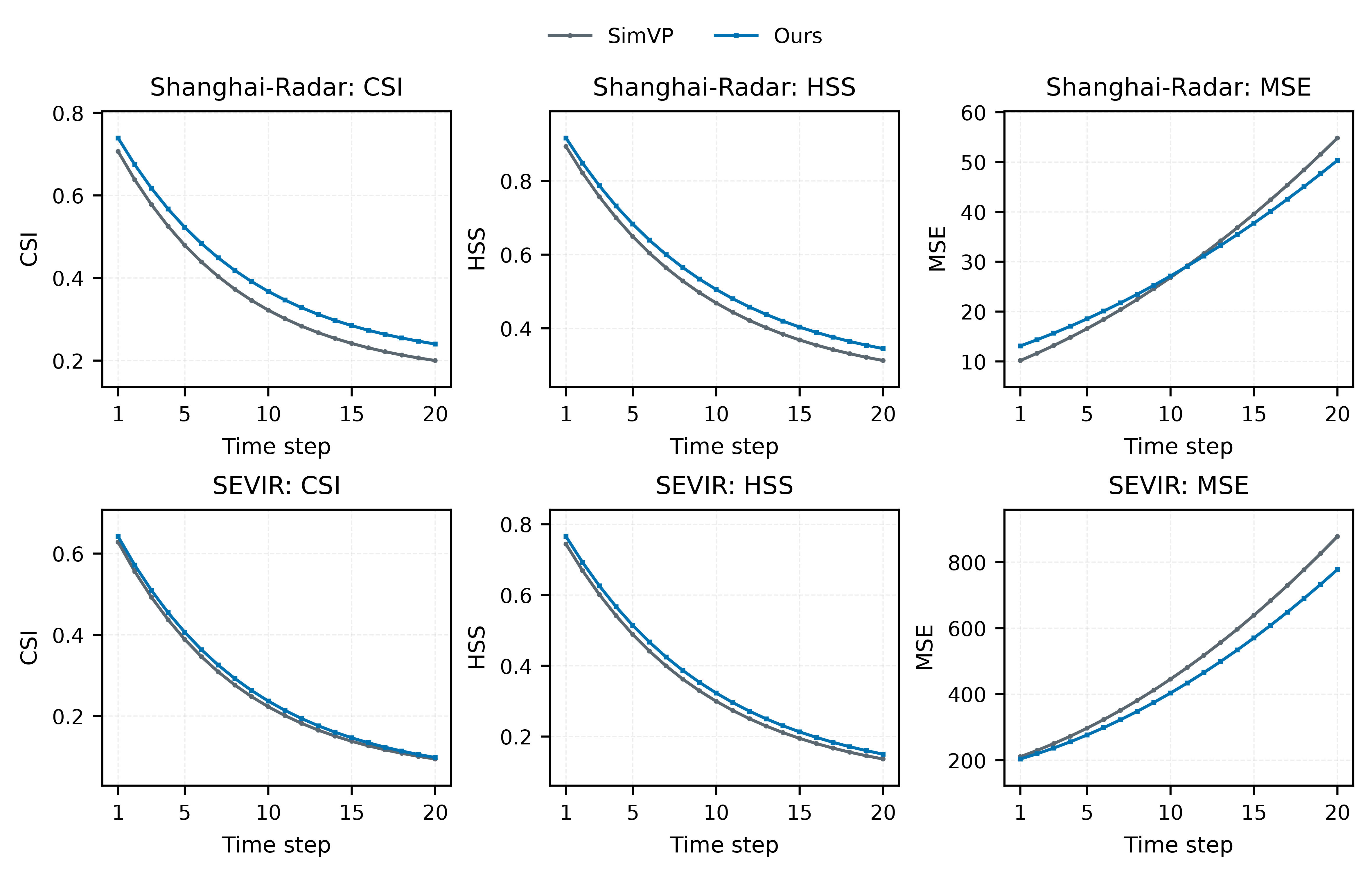
Figure 4. Lead-time-wise performance across all 20 forecast steps on Shanghai-Radar and SEVIR. Higher CSI and HSS are better, while lower MSE is better. MSE: Mean squared error.
4.8. Sensitivity to the temporal consistency weight
The temporal consistency weight
Sensitivity analysis of
| CSI | HSS | BS | TGE | SSIM | MSE | |
| Moderate temporal consistency improves coherence, while overly large values over-smooth adjacent predictions. Bold values indicate the best result for each metric. BS: Bias score; TGE: temporal gradient error; MSE: mean squared error. | ||||||
| 0 | 0.3876 | 0.5298 | 1.06 | 4.68 | 0.7758 | 29.5842 |
| 0.01 | 0.3941 | 0.5356 | 1.04 | 4.43 | 0.7786 | 29.5119 |
| 0.05 | 0.4002 | 0.5397 | 1.02 | 4.25 | 0.7813 | 29.4725 |
| 0.1 | 0.4038 | 0.5419 | 1.01 | 4.18 | 0.7824 | 29.4490 |
| 0.2 | 0.3994 | 0.5384 | 0.98 | 4.22 | 0.7807 | 29.6038 |
| 0.5 | 0.3916 | 0.5301 | 0.96 | 4.47 | 0.7742 | 30.0846 |
| 1.0 | 0.3769 | 0.5163 | 0.91 | 4.93 | 0.7628 | 31.2154 |
4.9. Efficiency comparison
Since real-time nowcasting systems require both accuracy and efficiency, we further compare model complexity and inference cost. The results in Table 6 show that the proposed model introduces almost no increase in parameter count, FLOPs, or inference time relative to the SimVP baseline, while increasing GPU memory usage because of the additional attention operations. Even with this overhead, the model stays competitive with most recurrent and transformer-based alternatives, so the added attention does not undermine the deployment advantages of the underlying backbone.
Efficiency comparison of representative methods
| Method | Params | FLOPs | Inference time (ms/sample) | FPS | GPU memory (MB) |
| FPS denotes the number of predicted samples per second during inference under the same hardware setting. Lower values are better for Params, FLOPs, inference time, and GPU memory. Higher values are better for FPS. Bold and underlined values indicate the best and second-best results for each efficiency metric, respectively. | |||||
| PhyDNet | 3.09M | 286.21G | 57.19 | 17.49 | 28.38 |
| PredRNN | 23.84M | 585.86G | 56.60 | 17.67 | 129.22 |
| PredRNN++ | 38.58M | 867.72G | 76.41 | 13.09 | 279.21 |
| SimVP | 14.87M | 95.94G | 182.03 | ||
| MAU | 7.63M | 103.43G | 110.57 | 9.04 | 230.52 |
| Tau | 11.74M | 82.89G | 24.79 | 40.34 | |
| Earthformer | 912.38K | 22.69G | 289.91 | 3.45 | 2904.55 |
| Ours | 14.87M | 95.94G | 49.84 | 20.06 | 246.87 |
5. DISCUSSION
The experiments indicate that CBAM-based feature refinement and TCR contribute in different ways. The gains in CSI and HSS point to CBAM helping the model concentrate on meteorologically informative echo regions, whereas the temporal consistency loss mainly improves the coherence of adjacent predictions. The two therefore address separate aspects of the nowcasting problem rather than reinforcing the same one.
The method also remains inexpensive relative to heavier recurrent and transformer-based alternatives. This matters for operational nowcasting, where inference speed and deployment simplicity often weigh as much as forecast quality. Because ConCast extends an efficient backbone instead of redesigning it, it keeps most of the computational advantage of SimVP while still improving accuracy.
The study also has several limitations. First, the method relies solely on radar-derived image sequences and does not incorporate auxiliary meteorological information such as wind fields, topography, or multi-source satellite observations. Second, the temporal consistency term is defined only between adjacent predictions and may therefore be insufficient for modeling longer-range temporal dependencies or uncertainty accumulation. Third, the current experiments focus on fixed-resolution inputs and benchmark settings; further evaluation under operational conditions, such as missing frames, domain shifts, and extreme precipitation events, would provide a more comprehensive assessment of robustness.
Future work may therefore explore multi-modal meteorological fusion, stronger physics-aware regularization, and uncertainty-aware forecasting objectives. It would also be valuable to investigate adaptive temporal regularization strategies and event-focused evaluation protocols for extreme rainfall nowcasting.
6. CONCLUSIONS
This study presented ConCast, an enhanced SimVP for precipitation nowcasting that integrates CBAM-based feature refinement with TCR. On the Shanghai-Radar and SEVIR datasets, it improved forecasting skill and structural quality over representative baselines while retaining most of the underlying backbone's efficiency.
These results indicate that pairing attention refinement with temporal regularization is a workable way to raise nowcasting quality without sacrificing efficiency.
DECLARATIONS
Authors' contributions
Made substantial contributions to the conception and design of the study, data analysis and interpretation, and drafting and revision of the manuscript: Zhao, P.; Wang, R.; Zhang, Y.; Yang, X.; Li, C.
All authors read and approved the final manuscript.
Availability of data and materials
The data supporting this study are publicly available. The Shanghai-Radar dataset is available from Harvard Dataverse at https://dataverse.harvard.edu/dataset.xhtml?persistentId=doi:10.7910/DVN/2GKMQJ and is also mirrored at https://drive.google.com/file/d/14JB4ElkZKHzqxIGKMFrbnY2P4zcae8RA/view. The SEVIR dataset is available at https://github.com/MIT-AI-Accelerator/neurips-2020-sevir, with an example tutorial at https://github.com/MIT-AI-Accelerator/eie-sevir/blob/master/examples/SEVIR_Tutorial.ipynb. SEVIR can also be downloaded from the public AWS S3 bucket according to the official instructions provided by the dataset authors.
AI and AI-assisted tools statement
During the preparation of this manuscript, the AI tool ChatGPT (GPT-5.5, released 2026-04-24) was used solely for language editing. The tool did not influence the study design, data collection, analysis, interpretation, or the scientific content of the work. All authors take full responsibility for the accuracy, integrity, and final content of the manuscript.
Financial support and sponsorship
This paper was funded by Natural Science Foundation of Shandong Province (No.ZR2025MS997).
Conflicts of interest
Zhao, P. is affiliated with China Energy Investment Corporation Co., Ltd., while the other authors have declared that they have no conflicts of interest.
Ethical approval and consent to participate
Not applicable.
Consent for publication
Not applicable.
Copyright
© The Author(s) 2026.
REFERENCES
1. Sun, J.; Xue, M.; Wilson, J. W.; et al. Use of NWP for nowcasting convective precipitation: recent progress and challenges. Bull. Am. Meteorol. Soc. 2014, 95, 409-26.
2. Liang, Q. Q.; Feng, Y. R.; Deng, W. J.; et al. A composite approach of radar echo extrapolation based on TREC vectors in combination with model-predicted winds. Adv. Atmos. Sci. 2010, 27, 1119-30.
3. Bechini, R.; Chandrasekar, V. An enhanced optical flow technique for radar nowcasting of precipitation and winds. J. Atmos. Ocean. Technol. 2017, 34, 2637-58.
4. Chen, M. X.; Qin, R.; Song, L. Y.; et al. SMART2022: a project supporting weather forecasting and services for the Beijing 2022 Olympic and Paralympic Winter Games - a success story of precise observations, accurate forecasting, and meticulous service in the field of meteorology. Bull. Am. Meteorol. Soc. 2025, 106, E1401-33.
5. Shi, X.; Chen, Z.; Wang, H.; Yeung, D. Y.; Wong, W.; Woo, W. Convolutional LSTM network: a machine learning approach for precipitation nowcasting. arXiv 2015, arXiv: 1506.04214. Available online: https://doi.org/10.48550/arXiv.1506.04214. (accessed 20 Jul 2026).
6. Shi, X.; Gao, Z.; Lausen, L.; et al. Deep learning for precipitation nowcasting: a benchmark and a new model. arXiv 2017, arXiv: 1706.03458. Available online: https://doi.org/10.48550/arXiv.1706.03458. (accessed 20 Jul 2026).
7. Wang, Y.; Long, M.; Wang, J.; Gao, Z.; Yu, P. S. PredRNN: recurrent neural networks for predictive learning using spatiotemporal LSTMs. In Proceedings of the 31st International Conference on Neural Information Processing Systems, 2017. Curran Associates Inc., 2017; pp. 879-88.
8. Wang, Y.; Gao, Z.; Long, M.; Wang, J.; Yu, P. S. PredRNN++: towards a resolution of the deep-in-time dilemma in spatiotemporal predictive learning. arXiv 2018, arXiv: 1804.06300. Available online: https://doi.org/10.48550/arXiv.1804.06300. (accessed 20 Jul 2026).
9. Wang, Y.; Zhang, J.; Zhu, H.; Long, M.; Wang, J.; Yu, P. S. Memory in memory: a predictive neural network for learning higher-order non-stationarity from spatiotemporal dynamics. In 2019 IEEE/CVF Conference on Computer Vision and Pattern Recognition (CVPR), Long Beach, USA, Jun 15-20, 2019. IEEE; 2019. pp. 9146-54.
10. Tang, S.; Li, C.; Zhang, P.; Tang, R. SwinLSTM: improving spatiotemporal prediction accuracy using swin transformer and LSTM. In 2023 IEEE/CVF International Conference on Computer Vision (ICCV), Paris, France, Oct 01-06, 2023. IEEE; 2023. pp. 13424-33.
11. Guen, V. L.; Thome, N. Disentangling physical dynamics from unknown factors for unsupervised video prediction. In 2020 IEEE/CVF Conference on Computer Vision and Pattern Recognition (CVPR), Seattle, USA, Jun 13-19, 2020. IEEE; 2020. pp. 11471-81.
12. Chang, Z.; Zhang, X.; Wang, S.; et al. MAU: a motion-aware unit for video prediction and beyond. In Proceedings of the 35th International Conference on Neural Information Processing Systems, 2021. Curran Associates Inc., 2021; pp. 26950-62.
13. Finn, C.; Goodfellow, I.; Levine, S. Unsupervised learning for physical interaction through video prediction. arXiv 2016, arXiv: 1605.07157. Available online: https://doi.org/10.48550/arXiv.1605.07157. (accessed 20 Jul 2026).
14. Lotter, W.; Kreiman, G.; Cox, D. Deep predictive coding networks for video prediction and unsupervised learning. arXiv 2016, arXiv: 1605.08104. Available online: https://doi.org/10.48550/arXiv.1605.08104. (accessed 20 Jul 2026).
15. Villegas, R.; Yang, J.; Hong, S.; Lin, X.; Lee, H. Decomposing motion and content for natural video sequence prediction. arXiv 2017, arXiv: 1706.08033. Available online: https://doi.org/10.48550/arXiv.1706.08033. (accessed 20 Jul 2026).
16. Denton, E.; Fergus, R. Stochastic video generation with a learned prior. arXiv 2018, arXiv: 1802.07687. Available online: https://doi.org/10.48550/arXiv.1802.07687. (accessed 20 Jul 2026).
17. Gao, Z.; Tan, C.; Wu, L.; Li, S. Z. SimVP: simpler yet better video prediction. arXiv 2022, arXiv: 2206.05099. Available online: https://doi.org/10.48550/arXiv.2206.05099. (accessed 20 Jul 2026).
18. Tan, C.; Gao, Z.; Wu, L.; Xu, Y.; Xia, J.; Li, S. Temporal attention unit: towards efficient spatiotemporal predictive learning. In 2023 IEEE/CVF Conference on Computer Vision and Pattern Recognition (CVPR), Vancouver, Canada, June 17-24, 2023. IEEE; 2023. pp. 18770-82.
19. Gao, Z.; Shi, X.; Wang, H.; et al. Earthformer: exploring space-time transformers for earth system forecasting. arXiv 2022, arXiv: 2207.05833. Available online: https://doi.org/10.48550/arXiv.2207.05833. (accessed 20 Jul 2026).
20. Sønderby, C. K.; Espeholt, L.; Heek, J.; et al. MetNet: a neural weather model for precipitation forecasting. arXiv 2020, arXiv: 2003.12140. Available online: https://doi.org/10.48550/arXiv.2003.12140. (accessed 20 Jul 2026).
21. Espeholt, L.; Agrawal, S.; Sønderby, C. K.; et al. Skillful twelve hour precipitation forecasts using large context neural networks. arXiv 2021, arXiv: 2111.07470. Available online: https://doi.org/10.48550/arXiv.2111.07470. (accessed 20 Jul 2026).
22. Pathak, J.; Subramanian, S.; Harrington, P.; et al. FourCastNet: a global data-driven high-resolution weather model using adaptive fourier neural operators. arXiv 2022, arXiv: 2202.11214. Available online: https://doi.org/10.48550/arXiv.2202.11214. (accessed 20 Jul 2026).
23. Bi, K.; Xie, L.; Zhang, H.; Chen, X.; Gu, X.; Tian, Q. Accurate medium-range global weather forecasting with 3D neural networks. Nature 2023, 619, 533-38.
24. Lam, R.; Sanchez-Gonzalez, A.; Willson, M.; et al. GraphCast: learning skillful medium-range global weather forecasting. arXiv 2022, arXiv: 2212.12794. Available online: https://doi.org/10.48550/arXiv.2212.12794. (accessed 20 Jul 2026).
25. Nguyen, T.; Brandstetter, J.; Kapoor, A.; Gupta, J. K.; Grover, A. ClimaX: a foundation model for weather and climate. arXiv 2023, arXiv: 2301.10343. Available online: https://doi.org/10.48550/arXiv.2301.10343. (accessed 20 Jul 2026).
26. Gong, J.; Bai, L.; Ye, P.; et al. CasCast: skillful high-resolution precipitation nowcasting via cascaded modelling. arXiv 2024, arXiv: 2402.04290. Available online: https://doi.org/10.48550/arXiv.2402.04290. (accessed 20 Jul 2026).
27. Babaeizadeh, M.; Finn, C.; Erhan, D.; Campbell, R. H.; Levine, S. Stochastic variational video prediction. arXiv 2017, arXiv: 1710.11252. Available online: https://doi.org/10.48550/arXiv.1710.11252. (accessed 20 Jul 2026).
28. Chang, Z.; Zhang, X.; Wang, S.; Ma, S.; Gao, W. STRPM: a spatiotemporal residual predictive model for high-resolution video prediction. In 2022 IEEE/CVF Conference on Computer Vision and Pattern Recognition (CVPR), New Orleans, USA, Jun 18-24, 2022. IEEE; 2022. pp. 13926-35.
29. Ravuri, S.; Lenc, K.; Willson, M.; et al. Skilful precipitation nowcasting using deep generative models of radar. Nature 2021, 597, 672-7.
30. Zhang, Y.; Long, M.; Chen, K.; et al. Skilful nowcasting of extreme precipitation with NowcastNet. Nature 2023, 619, 526-32.
31. Yu, D.; Li, X.; Ye, Y.; Zhang, B.; Luo, C.; Dai, K. DiffCast: a unified framework via residual diffusion for precipitation nowcasting. In 2024 IEEE/CVF Conference on Computer Vision and Pattern Recognition (CVPR), Seattle, USA, Jun 16-22, 2024. IEEE; 2024. pp. 27758-67.
32. Xu, W.; Chen, K.; Han, T.; Chen, H.; Ouyang, W.; Bai, L. ExtremeCast: boosting extreme value prediction for global weather forecast. arXiv 2024, arXiv: 2402.01295. Available online: https://doi.org/10.48550/arXiv.2402.01295. (accessed 20 Jul 2026).
33. Woo, S.; Park, J.; Lee, J. Y.; Kweon, I. S. CBAM: convolutional block attention module. In Proceedings of the European conference on computer vision (ECCV), 2018. Springer, Cham; 2018. pp. 3-19.
34. Ronneberger, O.; Fischer, P.; Brox, T. U-Net: convolutional networks for biomedical image segmentation. In Medical image computing and computer-assisted intervention - MICCAI 2015, Munich, Germany, Oct 05-09, 2015. Springer; 2015. pp. 234–41.
35. Ayzel, G.; Scheffer, T.; Heistermann, M. RainNet v1.0: a convolutional neural network for radar-based precipitation nowcasting. Geosci. Model. Dev. 2020, 13, 2631-44.
36. Agrawal, S.; Barrington, L.; Bromberg, C.; Burge, J.; Gazen, C.; Hickey, J. Machine learning for precipitation nowcasting from radar images. arXiv 2019, arXiv: 1912.12132. Available online: https://doi.org/10.48550/arXiv.1912.12132. (accessed 20 Jul 2026).
37. Wang, Q.; Wu, B.; Zhu, P.; Li, P.; Zuo, W.; Hu, Q. ECA-Net: efficient channel attention for deep convolutional neural networks. In 2020 IEEE/CVF Conference on Computer Vision and Pattern Recognition (CVPR), Seattle, USA, Jun 13-19, 2020. IEEE; 2020. pp. 11531-9.
38. Zhang, C.; Yan, Q.; Meng, L.; Sylvain, T. What constitutes good contrastive learning in time-series forecasting? arXiv 2023, arXiv: 2306.12086. Available online: https://doi.org/10.48550/arXiv.2306.12086. (accessed 20 Jul 2026).
39. Zheng, X.; Chen, X.; Schürch, M.; Mollaysa, A.; Allam, A.; Krauthammer, M. Simple contrastive representation learning for time series forecasting. arXiv 2023, arXiv: 2303.18205. Available online: https://doi.org/10.48550/arXiv.2303.18205. (accessed 20 Jul 2026).
40. Lai, W. S.; Huang, J. B.; Wang, O.; Shechtman, E.; Yumer, E.; Yang, M. H. Learning blind video temporal consistency. In Proceedings of the European Conference on Computer Vision (ECCV), 2018. Springer, Cham; 2018. pp. 179-95.
41. Dwibedi, D.; Aytar, Y.; Tompson, J.; Sermanet, P.; Zisserman, A. Temporal cycle-consistency learning. In 2019 IEEE/CVF Conference on Computer Vision and Pattern Recognition (CVPR), Long Beach, USA, Jun 15-20, 2019. IEEE; 2019. pp. 1801-10.
42. Guan, D.; Huang, J.; Xiao, A.; Lu, S. Domain adaptive video segmentation via temporal consistency regularization. In 2021 IEEE/CVF International Conference on Computer Vision (ICCV), Montreal, Canada, Oct 10-17, 2021. IEEE; 2021. pp. 8033-44.
43. Chen, L.; Cao, Y.; Ma, L.; Zhang, J. A deep learning-based methodology for precipitation nowcasting with radar. Earth. Space. Sci. 2020, 7, e2019EA000812.
Cite This Article
 Open Access
How to Cite
Download Citation
Export Citation File:
Type of Import
Tips on Downloading Citation
Citation Manager File Format
Type of Import
Direct Import: When the Direct Import option is selected (the default state), a dialogue box will give you the option to Save or Open the downloaded citation data. Choosing Open will either launch your citation manager or give you a choice of applications with which to use the metadata. The Save option saves the file locally for later use.
Indirect Import: When the Indirect Import option is selected, the metadata is displayed and may be copied and pasted as needed.
About This Article
Copyright

Data & Comments
Data
0










Comments
Comments must be written in English. Spam, offensive content, impersonation, and private information will not be permitted. If any comment is reported and identified as inappropriate content by OAE staff, the comment will be removed without notice. If you have any queries or need any help, please contact us at [email protected].