


Label co-occurrence guided nonlinear disambiguation for partial multi-label learning
 0
0 Abstract
Partial multi-label learning (PML) addresses challenges where each instance is associated with a set of candidate labels that includes both relevant and irrelevant ones. Traditional label disambiguation strategies often overlook the importance of nonlinear subspace structures. The assumption that data points closely adhere to multiple linear subspaces is restrictive and may not hold in certain applications. Linear subspace clustering algorithms frequently struggle with data that lie on multiple nonlinear manifolds, because they focus only on global linear relationships between data points. To address this gap, we propose a novel approach called label co-occurrence guided nonlinear disambiguation for partial multi-label learning (LCND). Specifically, we introduce a label weight-guided kernel low-rank representation to learn an instance affinity matrix in a nonlinear feature space, enabling effective identification of instances with complex nonlinear structures. Meanwhile, we design a weighted Jaccard distance to quantify label relevance by exploiting label frequency and co-occurrence information. By jointly optimizing instance-level and label-level affinity matrices, the proposed method effectively denoises labels under weak supervision. Extensive experimental results demonstrate that LCND significantly outperforms most state-of-the-art PML methods on the vast majority of benchmark datasets and evaluation metrics.
Keywords
1. INTRODUCTION
In the domain of supervised machine learning, multi-label learning (MLL) addresses situations where a single entity can be associated with multiple categories simultaneously[1-3]. Standard MLL algorithms typically require exhaustive label data for the training dataset[1], and it is imperative that each training sample be precisely annotated. However, accurately annotating such instances is extremely challenging. Because obtaining completely correct label annotations is time-consuming and labor-intensive[4-6], the collected labels are often incomplete, containing both correct and superfluous labels. This scenario has been defined as partial multi-label learning (PML) by[7].
To tackle the challenges of PML, employing multi-label classification techniques such as BR[8], ML-kNN[9], and CPLST[10] is a viable strategy. However, the presence of noisy labels in the candidate label set can severely distort the training process[3,11].
To address these challenges, various PML techniques have been proposed in recent years[12]. Many PML methods focus on exploiting the intrinsic properties of both the feature and label spaces. In the label decomposition process of PML-LRS[13], part of the label matrix is assumed to be a low-rank ground-truth label matrix, while the other part is treated as a sparse matrix of irrelevant labels. GLC[14] introduces a label coefficient matrix via low-rank representation (LRR) to capture the global structural information of labels from multiple subspaces. Some methods attempt to reduce the impact of noise in the feature matrix through low-rank and sparse decomposition schemes. Additionally, PML-NI[15] considers the origin of noisy labels, arguing that they typically stem from the ambiguity of instance content. PAMB[16] transforms the PML problem into multiple binary decomposition problems. However, these methods share a critical limitation: when jointly exploiting information from the instance and label spaces[17], they largely overlook the nonlinear subspace structures inherent in real-world data. Forcing features that reside in nonlinear subspaces to be modeled as linear can lead to inaccurate semantic spaces for instances or labels. Furthermore, the instance space and the label space are inherently strongly connected, yet the joint role of candidate labels and instances remains underexplored.
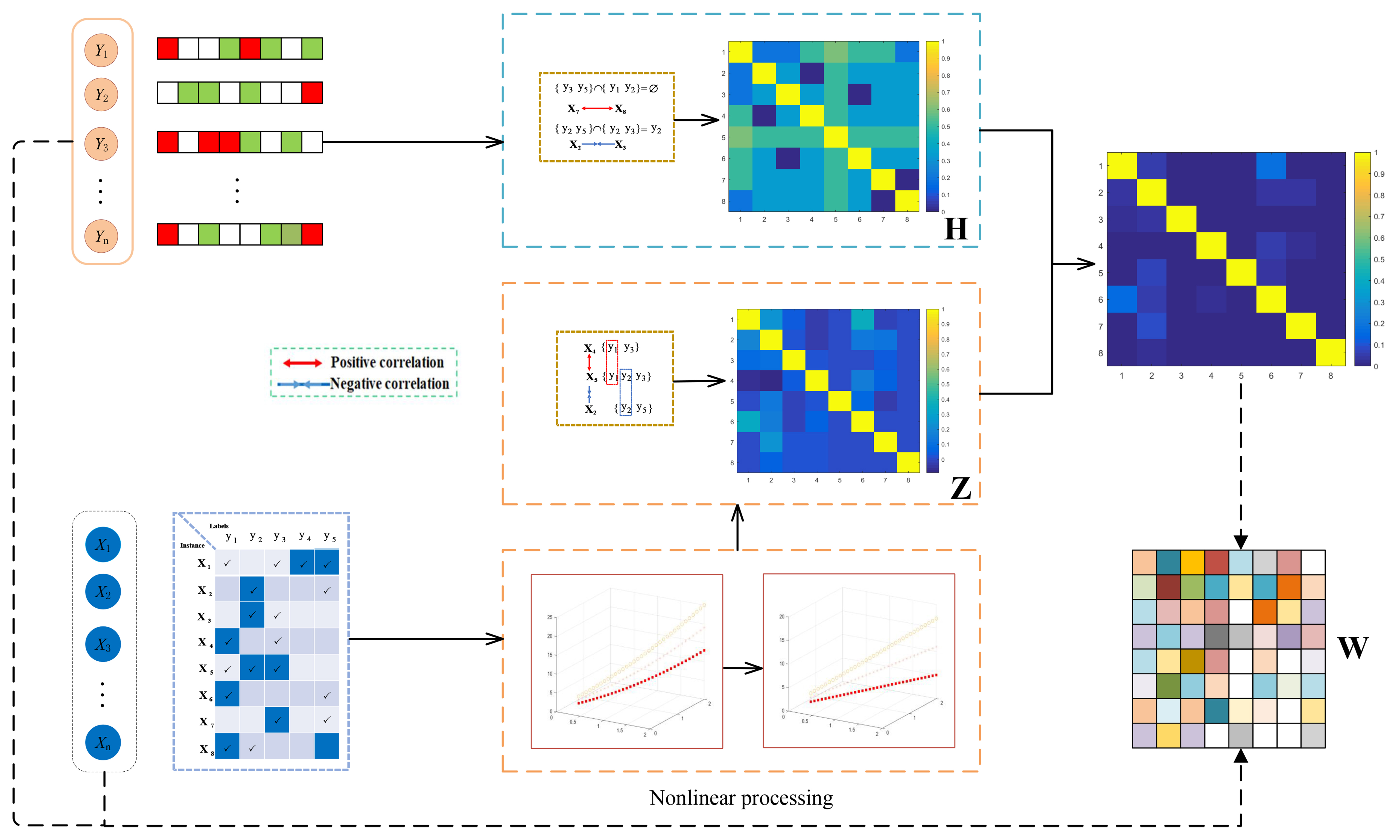
A new PML technique, designated as label co-occurrence guided nonlinear disambiguation for partial multi-label learning (LCND), has been introduced to solve the challenges outlined above. Recently, LRR[18,19] has garnered substantial interest due to its exceptional proficiency in subspace clustering. This approach assumes that high-dimensional data lie close to a union of several low-dimensional linear subspaces. Nonetheless, LRR may fail to produce optimal results with data originating from nonlinear subspaces, as it was initially designed for handling linear subspaces within the input domain[20]. Certain PML techniques that leverage LRR attempt to resolve label ambiguities by decomposing the candidate label matrix into an ideal component and a noise-based component[13]. However, this approach fails to capture the nonlinear interconnections of the data, leading to a loss of local data features and similarity cues during the learning process. Meanwhile, it has been demonstrated that nonlinear subspace learning significantly enhances similarity estimation, as supported by[21]. Numerous researchers have integrated nonlinear subspaces into their studies to demonstrate their effectiveness. Tanfous et al. proposed that suitable shape representations and their temporal evolution, termed trajectories, often lie on nonlinear manifolds[22]. Roweis et al. introduced locally linear embedding (LLE) by exploiting the local symmetries of linear reconstructions[23]. Using this methodology, LLE can discern the overarching structure of nonlinear manifolds. Conventional linear subspace clustering techniques frequently encounter difficulties when processing data that span multiple nonlinear manifolds. Such challenges are expected, as these methodologies primarily account for global linear correlations among data points. In the context of nonlinear manifolds, the intricate local interactions among data points play a more significant role[24]. Inspired by this research, to overcome the limitations of linear models, we employ a kernel-based mapping technique to project data from the original input space into a feature space using the robust kernel low-rank representation (RKLRR)[20] method. In this transformed feature space, data points are likely to be distributed across various linear subspaces. Subsequently, we can derive an instance affinity matrix, ensuring that instances sharing the same labels lie in the same subspace. In our study, we propose a novel label disambiguation method that incorporates the Jaccard distance to measure similarity between candidate labels, thereby constructing a label affinity matrix. Furthermore, we demonstrate that by integrating this matrix with an instance affinity matrix, our approach effectively harnesses complementary information, thereby enhancing the accuracy and reliability of the label disambiguation.
To summarize our findings, this research makes several key contributions:
1. We propose a novel method for learning instance affinity matrices by exploring nonlinear subspace data and candidate label information. Using kernel methods for high-dimensional mapping, this approach effectively identifies instances that share the same label, even when the original nonlinear subspace data cause them to lie in multiple linear subspaces.
2. We design a weighted Jaccard distance for label affinity modeling, where label weights are adaptively learned based on label frequency and co-occurrence statistics. This method captures implicit label hierarchies without requiring additional annotations, thereby improving label denoising accuracy.
3. We develop a joint optimization framework for instance-level and label-level affinity matrices, fully leveraging their complementary information to address the insufficient joint utilization of label and instance data in existing PML methods.
2. RELATED WORK
2.1. Partial label learning
In the field of weakly supervised learning, partial label learning (PLL)[25-27] differs from both supervised and unsupervised learning. Its core objective is to identify a single ground-truth label for each instance from a set of candidate labels[28]. In PLL, each candidate label set contains exactly one ground-truth label and several noisy labels. Existing PLL methods can be categorized into three strategies: label disambiguation, label transformation, and theory-driven methods.
Label disambiguation techniques primarily include mean-based methods and recognition-based methods[29]. One type of mean-based method[30] proposes a convex optimization approach, where predictions are obtained by averaging the model outputs over all candidate labels. Another method performs vote aggregation on the candidate label sets of neighboring samples of unseen instances[31-33]. Recognition-based PLL methods[34-36] treat the ground-truth label as a latent variable and infer the most probable label by constructing a parametric model. In recent years, this approach has been integrated with advanced representation learning techniques such as contrastive learning[37] and graph neural networks[38].
The label transformation strategy[39,40] aims to mitigate the impact of false-positive labels on the candidate set. Theory-driven methods focus on the theoretical foundations of PLL, addressing core issues such as statistical consistency[41-43]. Additionally, PLL research has been extended to scenarios including class imbalance, multi-view learning, online learning, high-dimensional data, and dimensionality reduction.
The essence of label disambiguation lies in extracting ground-truth label information by evaluating the credibility of candidate labels. Furthermore, PML significantly increases problem complexity, as the number of ground-truth labels in each candidate label set is unknown, whereas PLL assumes a single ground-truth label.
2.2. PML
PML addresses the scenario in which each training instance is annotated with a candidate label set that contains both ground-truth labels and irrelevant noisy labels[7]. A naive strategy is to treat all candidate labels as correct and apply conventional MLL algorithms such as ML-KNN[9]. However, the presence of noisy labels severely degrades the performance of such approaches. To overcome this limitation, numerous PML methods have been developed, which can be broadly categorized into two paradigms: two-stage disambiguation methods (TDM) and unified framework methods (UFM).
2.2.1. TDM
TDM first identify highly reliable labels from the candidate set and subsequently train a robust multi-label classifier using the refined label confidences. Xie and Huang introduced PML-lc and PML-fp, which estimate the probability of each candidate label being ground-truth by exploiting feature-level label correlations and then rank the most relevant labels for each instance[7]. Zhang and Fang proposed PARTICLE, which extracts credible labels through iterative label propagation and then builds a multi-label predictor via pairwise label ranking with virtual label splitting and maximum a posteriori inference[44]. Wang et al. developed DRAMA, which constructs a label confidence matrix using feature manifolds and learns a gradient-boosted model to fit these confidences, augmenting the feature space with previous label predictions to capture higher-order label correlations[45]. Liu et al. presented PAMB, which leverages error-correcting output codes to decompose the PML problem into multiple binary classification tasks, thereby avoiding direct label confidence estimation and employing a loss-weighted decoding strategy for prediction[16].
Despite their effectiveness, two-stage methods suffer from an inherent limitation: errors introduced in the first stage can propagate to the second stage. This issue becomes particularly acute in datasets with high label-noise ratios, where inaccurate confidence estimates may undermine the entire learning process.
2.2.2. UFM
In contrast to two-stage approaches, UFM integrate label disambiguation and model training into a single optimization process, iteratively refining the estimates of ground-truth labels during learning. A prominent line of research within this category assumes that the intrinsic relationships between labels and features can be captured in a low-rank subspace, thereby filtering out label noise[13,14,46]. Sun et al. proposed PML-LRS, which decomposes the candidate label matrix into a low-rank ground-truth component and a sparse noise component, and jointly learns a prediction model[13]. Sun et al. further introduced GLC, which integrates global label structures and global-local correlations to enhance disambiguation[14]. Yu et al. proposed fPML, which assumes that labels and features reside in a unified space where noise is naturally eliminated through LRR[46]. Xie and Huang developed PML-NI, a unified framework that simultaneously recovers ground-truth labels and identifies noisy ones by exploiting label correlations via trace norm and ℓ1 norm regularizers, while also modeling noise directly from feature information[15]. Gong et al. proposed MILI-PML, which identifies genuine labels through mutual information maximization[47].
Additional studies have explored complementary directions within unified frameworks. Wu et al. proposed FIMAN, which enhances feature representation and label precision by leveraging the geometry of multi-view datasets[48]. Hao et al. formulated PML-FSOS as a feature selection problem in the presence of noise, jointly examining the label and feature spaces[49]. Hang and Zhang introduced PARD, which pioneers the use of probabilistic graphical models for PML disambiguation[50]. Wang et al. proposed PML-ED, which uses KNN-based label attention for probabilistic distribution estimation and conditional layer normalization to capture higher-order label correlations. Recently, deep learning-based PML methods have also emerged[51]. Li et al. proposed PML-KGT, which incorporates a K-means graph transformer, cluster centers, and a class-aware correction loss to mitigate the effects of noisy labels[52].
However, despite substantial progress, most existing PML methods still assume that data lie in linear subspaces, whereas real-world data often exhibit complex nonlinear structures. Moreover, the joint exploitation of label correlations and instance-level relationships remains insufficiently explored. These limitations motivate the development of our proposed LCND framework, which integrates kernel-based nonlinear feature mapping with weighted label affinity constraints to achieve robust label disambiguation.
3. THE PROPOSED APPROACH
In this section, we detail the formulation and implementation of LCND, which extends prior work[53] to address the nonlinear PML problem while accounting for label frequency information.
We represent the feature matrix as X = [x1, x2, …, xn] ∈ ℝd×n, where d denotes the dimensionality of the feature vectors and n is the total number of instances. The matrix Y = [y1, y2, …, yn] ∈ ℝm×n captures the label assignments for the labeled samples, where m is the total number of distinct labels. An entry yji = 1 indicates that the instance xi is annotated with the j-th label, while yji = 0 indicates the absence of that label.
To predict labels for unseen instances, we learn a projection matrix W = [w1, w2, …, wd] ∈ ℝm×d that maps feature representations to the label space. Consequently, we optimize W by minimizing the quadratic loss as follows:
In this context, we add a squared Frobenius norm penalty to regularize W, which helps prevent overfitting, where β is a balancing parameter.
3.1. Learn nonlinear relationships
LRR[54,55] addresses the subspace clustering problem by identifying the inherent subspace structures of the dataset X. The objective of LRR is to find a minimal-rank approximation of X using a suitable dictionary[18], which can be formulated as follows:
Here, λ > 0 is a regularization parameter, E ∈ ℝd×n represents the reconstruction error, ||Z||* denotes the nuclear norm, and ||E||2,1 = Σj=1n(Σi=1d(Eij)2)1/2. The matrix Z, obtained by solving Equation (2), approximates a block-diagonal form, where instances with high similarity are grouped into the same subspace, and the magnitudes of the representation coefficients for similar instances are relatively large.
The equality constraint in Equation (2) can be rewritten as E = X - XZ. Consequently, the LRR optimization problem defined in Equation (2) is equivalent to the following formulation:
Introducing an auxiliary matrix P = I - Z ∈ ℝn×n allows us to express ||X - XZ||2,1 from Equation (2) as ||X - XZ||2,1 = ||X(I - Z)||2,1 = ||XP||2,1 = Σi=1n||Xpi|| = Σi=1n(piTXTpi)1/2, with P = [p1, …, pn], where pi ∈ ℝn is the i-th column vector of P for i = 1, …, n. Therefore, the formulation in Equation (3) can be reformulated as:
After this reformulation, once the LRR formulation in Equation (2) is transformed into Equation (4), the dataset {xi}i=1n is represented solely through inner products (i.e., xiTxj) within the expression XTX. This property naturally allows the incorporation of kernel methods. Specifically, the subsequent nonlinear adaptation of LRR is obtained by substituting X in Equation (2) with Ψ(X):
Within this framework, Ψ(X) = [Ψ(x1), …, Ψ(xn)] denotes the feature mapping, with Ψ being the transformation Ψ: ℝd →
where pi ∈ ℝn is the i-th column vector of P for i = 1, …, n. Then Equation (5) can be reformulated as:
The kernel matrix K, incorporated into g(P), plays a crucial role. It is worth noting that using a linear kernel, i.e., K = XTX, reduces the formulation in Equation (7) to that of Equation (2), making LRR a special case of linear kernel methods. Kernel techniques facilitate the detection of complex nonlinear patterns and interactions in the dataset. This is achieved by projecting the data from the original space into a Reproducing Kernel Hilbert Space (RKHS), thereby improving the representation for the target task. With the kernel, nonlinear data structures can be effectively mapped to linearly separable subspaces in the feature space. Consequently, this allows for a comprehensive assessment of similarity between instances. Dissimilar instances, in contrast, are assigned to different subspaces with minimal cross-representation values. As a result, the learned LRR captures instance similarity, where a larger zij indicates a stronger affinity between xi and xj.
3.2. Learning label affinity matrix
In PML, exploiting inter-instance relationships can facilitate more accurate label disambiguation. For example, if similarity assessment is based solely on feature distance, instances xi and xj might appear similar[56,57], yet they could belong to different classes due to the empty intersection of their label sets, i.e., Si ∩ Sj = Ø. Therefore, incorporating candidate label information helps mitigate the influence of feature-based nearest neighbors with inconsistent labels. Additionally, when instances have overlapping labels but dissimilar features, excluding these shared labels can aid the disambiguation process.
However, the standard Jaccard similarity treats all labels equally and ignores the implicit label hierarchy commonly observed in real-world datasets. To address this limitation, we propose a weighted Jaccard distance that incorporates label weights derived from the label data itself, without requiring additional prior knowledge.
Given the label matrix Y, we calculate the weight ωj of each label j (j = 1, 2, …, m) based on two statistical properties of the matrix. First, we consider the label frequency fj, which is the number of instances annotated with label j and corresponds to the sum of the j-th row of Y, i.e., fj = Σi=1nYj,i. We define the frequency score as:
Next, we introduce the label co-occurrence rate, which represents the proportion of other labels that co-occur with label j (i.e., labels that are simultaneously 1 with j in at least one instance). To compute this rate, we first construct the co-occurrence matrix Co ∈ ℝm×m, where Coj,k = Σi=1nYj,i × Yk,i denotes the number of instances in which labels j and k co-occur. We denote the co-occurrence rate as csc,j, and it is calculated as:
The final label weight is obtained by combining the frequency score and the co-occurrence rate using a balancing parameter η. We first compute the initial weight as initial_ωj = η·fsc,j + (1 - η)·csc,j, and then normalize these initial weights so that they sum to one, resulting in
Using the label weights ωj, we define the weighted Jaccard distance between label sets Si and Sj (where Si denotes the set of labels associated with instance i) as:
Compared with the standard Jaccard distance, the weighted variant emphasizes informative labels while suppressing the influence of rare or noisy labels.
Finally, the label affinity matrix H = [hij]n×n is defined as:
where hij represents the likelihood that instances xi and xj share ground-truth labels.
Notably, the label weights ωj and the label weight similarity simω(i, j) defined in this section are further integrated with the Gaussian kernel to construct a label weight-guided fused kernel matrix K, which underpins the subsequent nonlinear LRR. The formal definition of K is:
where θ balances the feature and label similarity, and γ > 0 is the Gaussian kernel bandwidth. K is positive semi-definite, ensuring compatibility with the low-rank optimization framework. Specifically, simω(i, j) quantifies label-based instance relevance and is computed as:
3.3. Predictor
Specifically, the intrinsic information present in potential label data can enhance the accuracy of subspace clustering. For instance, instances xi and xj may be distinct due to the absence of shared labels, i.e., Si ∩ Sj = Ø. Consequently, the corresponding zij values for these instances are forced to be negligible, either zero or nearly so. Based on this rationale, we incorporate a novel term ||Z○H||12[58], which integrates the potential label information, where H ∈ ℝn×n represents the label affinity matrix.
By combining the above components, LCND is defined as follows:
where α is a regularization parameter that controls the strength of the weak supervision constraint. Specifically, after obtaining the optimal projection matrix W through training, the predicted label vector for an unseen test sample xt is generated as yt = Wxt. The final label set is then determined by applying a threshold or by selecting the labels with the highest confidence scores.
3.4. Solving the optimization problem
Introducing auxiliary variables J, U, and V allows us to restructure the objective function in Equation (14) as follows:
The augmented lagrange multiplier (ALM) method[59] is then employed to handle the following augmented Lagrangian function:
where Y1, Y2, Y3, and Y4 are all N × N matrices in ℝN×N and serve as the Lagrange multipliers. Additionally, μ > 0 is a penalty parameter.
The optimization problem in Equation (11) can be solved iteratively by alternating minimization over the following subproblems:
(1) Optimize W while holding other parameters constant: With V, J, Z, U, and P fixed, the update equation for W is obtained by differentiating Equation (17):
This corresponds to a standard linear regression problem, whose solution can be determined as follows:
(2) Optimize V while holding other parameters constant: The task of updating V can be treated as a standard linear regression problem, and its solution can be expressed as:
(3) Optimize J while holding other parameters constant: With W, V, Z, U, and P fixed, the optimization of Equation (16) with respect to J reduces to the following problem:
The objective in Equation (20) can be equivalently written as:
Optimizing the objective function in Equation (21) involves performing singular value decomposition (SVD) on the matrix Z + Y2/μ, followed by applying soft thresholding to the resulting singular values.
(4) Optimize Z while holding other parameters constant: This is an ordinary least squares regression problem. Its solution is:
(5) Next, update U with the other variables fixed:
Therefore, U can be updated using Equation (24):
where the function
(6) Update P with the other variables fixed: The optimization problem for updating Pk+1 is formulated as follows:
where Ck+1 = I - Zk+1 + Y1,k/μk. Note that solving the problem in Equation (25) is nontrivial, as the objective function is convex but nonsmooth. Let ci (respectively, pi) denote the i-th column vector of C (respectively, P), and set the scalar τ = μk/λ. Then (μk/2)||P - C||F2 can be rewritten as μk((τ/2)Σi=1n||pi - ci||2). Normalizing the objective function by λ, the problem stated in Equation (25) can be reformulated as:
The problem can be decomposed into n independent subproblems, each taking the following form:
Lemma 1: Let τ > 0 be a scalar, b ∈ ℝq a constant vector (q is a positive integer), and S = diag({si}1≤i≤q) ∈ ℝq×q a diagonal matrix whose diagonal entries si are positive and sorted in descending order. Then the optimal solution p* to the following problem:
is given by
Here, S-1 = diag({si-1}1≤i≤q) is the inverse of S, and the positive scalar δ satisfies:
In particular, when ||S-1b|| > 1/τ, Equation (30) (with respect to δ) has a unique positive solution, which can be found via the bisection method as described in[20]. The proof of Lemma 1 is provided in the Supplementary Materials. Leveraging Lemma 1, we obtain the following theorem.
Theorem 1: For τ > 0, the optimal solution pi* to the problem in Equation (27) can be expressed as:
where
Here, δ is a positive scalar satisfying:
Specifically, if the norm ||[1/σ1, …, 1/
For a detailed update procedure, please refer to Algorithm 1. The detailed update process for parameter P is presented in Algorithm 2.
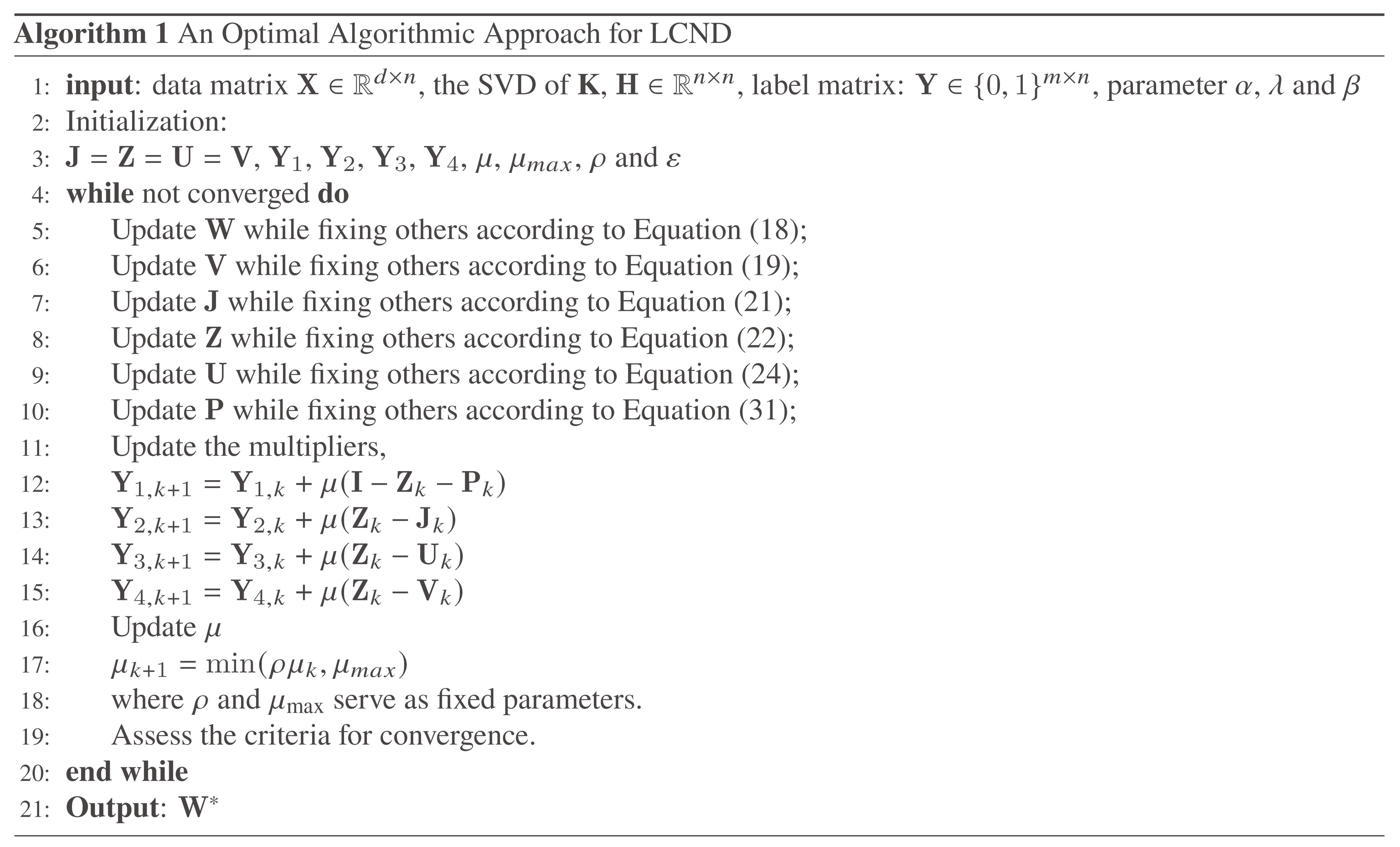
Algorithm 1.
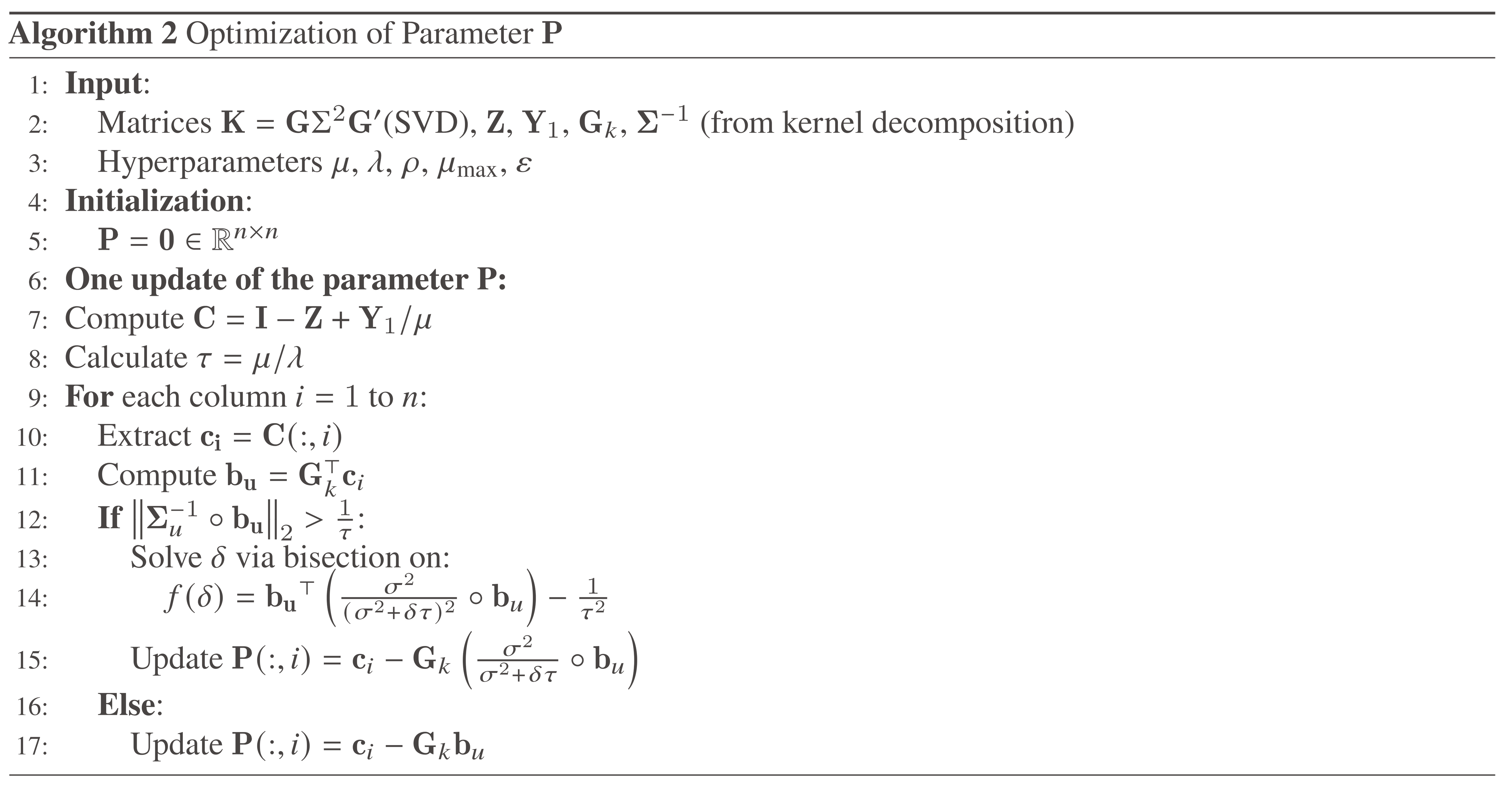
Algorithm 2.
4. EXPERIMENTS
In this study, we conduct experiments on three real-world datasets and six synthetic datasets to demonstrate the effectiveness of the proposed LCND algorithm. This section begins with an overview of the datasets, evaluation metrics, and compared algorithms. We then present four sets of experiments designed to verify the efficacy of LCND. First, we provide a comprehensive analysis of the results from eight different methods across 21 datasets. Second, we perform ablation studies to assess the contribution of handling nonlinear challenges and leveraging label correlations in our model. Third, we evaluate the model’s sensitivity to parameter variations. Finally, we analyze the computational complexity.
4.1. Datasets
We select three real-world datasets, namely music_emotion, music_style[44], and mirflickr[60]. As shown in Table 1, these datasets represent real-world PML instances, where candidate labels are obtained from online users and subsequently verified to establish ground-truth labels. In addition, we consider six synthetic datasets derived from multi-label benchmarks: Bibtex[61], Birds[62], Emotions[63], Image[9], Medical[64], and Scene[8]. To evaluate the robustness of our approach under different levels of label noise, we introduce a parameter r ∈ {1, 2, 3} that controls the number of false positive labels added to the candidate label set of each instance[16]. By applying these three noise settings to each of the six original multi-label datasets, we construct 6 × 3 = 18 synthetic PML datasets with varying noise intensities. In addition to these synthetic datasets, we also use the three real-world datasets for validation. All comparative experiments are therefore conducted across 21 benchmark datasets. The detailed characteristics of these datasets are summarized in Table 2.
Characteristics of the experimental data sets
| Data | Examples | Features | Labels | AVG*CL | AVG*GL |
| music_emotion | 6,833 | 98 | 11 | 5.29 | 2.42 |
| music_style | 6,839 | 98 | 10 | 6.04 | 1.44 |
| mirflickr | 10,433 | 100 | 7 | 3.35 | 1.77 |
Multi-label data sets employed to generate synthetic PML data sets
| Data | Examples | Features | Labels | AVG*CL | Configurations |
| Bibtex | 7,395 | 1,836 | 159 | 2.40 | r ∈ {1,2,3} |
| Birds | 645 | 260 | 19 | 1.01 | |
| Emotions | 593 | 72 | 6 | 1.87 | |
| Image | 2,000 | 294 | 5 | 1.24 | |
| Medical | 978 | 1,449 | 45 | 1.25 | |
| Scene | 2,407 | 294 | 6 | 1.08 |
4.2. Experimental setup
4.2.1. Evaluation metrics
To evaluate the performance of the eight compared algorithms, we adopt five widely used evaluation metrics: ranking loss, Hamming loss, one error, coverage, and average precision. For a comprehensive understanding of these metrics, refer to[1]. These metrics provide a multifaceted assessment of partial multi-label classification models. Specifically, performance improves as the values of ranking loss, Hamming loss, one error, and coverage decrease. Conversely, for average precision, a higher value indicates better performance. In addition, we use the microF1 metric[16]. LCND also achieves the best performance in terms of microF1. To evaluate the statistical significance of the performance differences between LCND and the best-performing baseline method, we conduct t-tests at the 0.05 significance level. The best results are highlighted in bold in the result tables.
4.2.2. Comparison with other methods
To evaluate the effectiveness of the proposed LCND approach, we compare it with seven state-of-the-art PML methods and one MLL method. The methods compared are listed as follows:
• ML-KNN[9] adapts the k-nearest neighbors approach for multi-label classification. It uses statistical information from the labels of the nearest training examples to predict label sets for unseen instances via a maximum a posteriori decision rule [suggested configuration: k = 10].
• PML-lc[7] optimizes the label relevance order for each instance by minimizing a rank loss weighted by confidence values, which estimate the likelihood that a candidate label is a ground-truth label. It refines these confidence values by exploiting structural information in the feature and label spaces [suggested configuration: C1 = 1, C2 = 1].
• PARTICLE[44] handles noisy and overcomplete candidate label sets using a two-stage process. It first identifies credible labels through label propagation and then induces a reliable multi-label predictor based on these labels [suggested configuration: k = 10, α = 0.95, thr = 0.9].
• PAMB[16] learns by transforming the PML problem into multiple binary classification tasks using error-correcting output codes. It avoids direct estimation of label confidence and instead employs a loss-weighted decoding strategy for prediction [suggested configuration: L = 100log2(q)].
• PML-NI[15] addresses PML by simultaneously recovering ground-truth labels and identifying noisy labels. It uses a unified optimization framework that exploits label correlations and directly models feature noise [suggested configuration: β = 0.5, γ = 0.5, λ = 1].
• NATAL[65] handles PML by assuming that the given labeling information is precise, and that missing feature information can be completed. It directly learns a prediction model from the enhanced features while considering all candidate labels [suggested configuration: α = 1, β = 10-6, λ = 0.1].
• PLAIN[66] leverages deep learning and graph techniques to disambiguate candidate label sets in PML. It uses instance-level and label-level similarities to improve label prediction accuracy [suggested configuration: K = 10, α = 0.01, β = 0.01, n = 0.1, ρ = 3].
• PML-TF[67] is an effective transformer-based framework for PML. It introduces partial K-means cross-attention to learn discriminative label embeddings and capture local features, and designs a class-aware correction loss to mitigate label noise [suggested configuration: γ = 2].
4.3. Performance comparison
The experimental work presented herein was conducted on a computing platform equipped with an octa-core processor (each core running at 2.0 GHz) and 16.0 GB of RAM. The software used for these experiments is MATLAB version R2016a.
The detailed experimental results are presented in Tables 3-6. In these tables, bold text indicates that the corresponding algorithm achieved the best performance among all compared methods. Compared with the competing methods, LCND achieves superior performance in most experimental settings. PLAIN outperforms LCND in only one case, namely on the Birds dataset with respect to ranking loss.
Compare LCND with PML methods on real data
| Data | LCND | ML-KNN | PML-lc | PARTICLE | PAMB | PML-NI | NATAL | PLAIN | PML-TF |
| Hamming Loss (the lower the better) | |||||||||
| music-emotion | 0.208±0.010 | 0.889±0.024 | 0.241±0.006 | 0.243±0.009 | 0.208±0.021 | 0.257±0.025 | 0.877±0.027 | 0.281±0.018 | 0.498±0.027 |
| music-style | 0.141±0.021 | 0.855±0.028 | 0.153±0.023 | 0.137±0.035 | 0.123±0.031 | 0.154±0.028 | 0.493±0.035 | 0.361±0.011 | 0.269±0.014 |
| mirflickr | 0.210±0.019 | 0.761±0.115 | 0.209±0.012 | 0.228±0.022 | 0.164±0.035 | 0.228±0.018 | 0.381±0.014 | 0.236±0.026 | 0.239±0.033 |
| Ranking Loss (the lower the better) | |||||||||
| music-emotion | 0.228±0.006 | 0.372±0.012 | 0.389±0.002 | 0.336±0.014 | 0.234±0.021 | 0.247±0.028 | 0.294±0.009 | 0.298±0.034 | 0.233±0.032 |
| music-style | 0.134±0.011 | 0.235±0.017 | 0.699±0.025 | 0.351±0.024 | 0.152±0.033 | 0.133±0.043 | 0.302±0.051 | 0.260±0.037 | 0.126±0.017 |
| mirflickr | 0.107±0.003 | 0.197±0.022 | 0.199±0.021 | 0.188±0.018 | 0.136±0.016 | 0.134±0.025 | 0.251±0.017 | 0.196±0.014 | 0.115±0.009 |
| One Error (the lower the better) | |||||||||
| music-emotion | 0.386±0.015 | 0.600±0.005 | 0.623±0.003 | 0.587±0.005 | 0.403±0.008 | 0.453±0.013 | 0.527±0.012 | 0.453±0.022 | 0.388±0.038 |
| music-style | 0.333±0.021 | 0.403±0.021 | 0.495±0.002 | 0.419±0.031 | 0.367±0.017 | 0.341±0.019 | 0.578±0.024 | 0.542±0.028 | 0.291±0.025 |
| mirflickr | 0.268±0.030 | 0.459±0.034 | 0.269±0.005 | 0.165±0.009 | 0.357±0.014 | 0.275±0.021 | 0.547±0.025 | 0.157±0.031 | 0.273±0.038 |
| Coverage (the lower the better) | |||||||||
| music-emotion | 0.394±0.009 | 0.568±0.015 | 0.521±0.023 | 0.484±0.009 | 0.412±0.023 | 0.408±0.025 | 0.492±0.043 | 0.412±0.019 | 0.443±0.029 |
| music-style | 0.195±0.013 | 0.302±0.007 | 0.467±0.011 | 0.368±0.005 | 0.213±0.012 | 0.191±0.023 | 0.352±0.013 | 0.405±0.017 | 0.256±0.021 |
| mirflickr | 0.211±0.007 | 0.285±0.009 | 0.224±0.022 | 0.305±0.032 | 0.237±0.016 | 0.235±0.032 | 0.317±0.011 | 0.284±0.014 | 0.215±0.021 |
| Average Precision (the higher the better) | |||||||||
| music-emotion | 0.628±0.006 | 0.525±0.024 | 0.489±0.003 | 0.542±0.007 | 0.636±0.013 | 0.612±0.012 | 0.581±0.021 | 0.612±0.034 | 0.596±0.009 |
| music-style | 0.747±0.008 | 0.654±0.123 | 0.523±0.052 | 0.621±0.073 | 0.722±0.023 | 0.743±0.059 | 0.548±0.046 | 0.580±0.037 | 0.741±0.018 |
| mirflickr | 0.810±0.011 | 0.685±0.008 | 0.675±0.034 | 0.690±0.028 | 0.768±0.028 | 0.781±0.048 | 0.660±0.062 | 0.768±0.033 | 0.805±0.017 |
| microF1 (the higher the better) | |||||||||
| music-emotion | 0.489±0.022 | 0.308±0.011 | 0.294±0.006 | 0.332±0.011 | 0.463±0.009 | 0.459±0.012 | 0.287±0.029 | 0.463±0.013 | 0.469±0.012 |
| music-style | 0.591±0.013 | 0.401±0.017 | 0.355±0.010 | 0.519±0.018 | 0.575±0.017 | 0.552±0.029 | 0.390±0.024 | 0.488±0.026 | 0.588±0.023 |
| mirflickr | 0.701±0.026 | 0.382±0.012 | 0.582±0.013 | 0.613±0.026 | 0.681±0.042 | 0.675±0.027 | 0.543±0.031 | 0.668±0.022 | 0.669±0.034 |
Comparison of LCND with state-of-the-art PML methods on six evaluation metrics
| Data | LCND | ML-KNN | PML-lc | PARTICLE | PAMB | PML-NI | NATAL | PLAIN | PML-TF |
| Hamming Loss (the lower the better) | |||||||||
| Bibtex | 0.014±0.002 | 0.998±0.012 | 0.018±0.034 | 0.015±0.006 | 0.024±0.018 | 0.014±0.048 | 0.982±0.071 | 0.012±0.037 | 0.014±0.003 |
| Birds | 0.055±0.006 | 0.997±0.032 | 0.056±0.053 | 0.164±0.027 | 0.141±0.029 | 0.062±0.014 | 0.901±0.019 | 0.053±0.034 | 0.121±0.046 |
| Emotions | 0.243±0.120 | 0.679±0.021 | 0.417±0.027 | 0.251±0.041 | 0.226±0.023 | 0.287±0.073 | 0.796±0.052 | 0.281±0.032 | 0.263±0.037 |
| Image | 0.182±0.017 | 0.849±0.033 | 0.213±0.031 | 0.754±0.029 | 0.208±0.015 | 0.209±0.013 | 0.826±0.018 | 0.967±0.023 | 0.241±0.016 |
| Medical | 0.010±0.001 | 0.984±0.071 | 0.012±0.042 | 0.012±0.042 | 0.034±0.045 | 0.012±0.017 | 0.971±0.024 | 0.017±0.052 | 0.011±0.018 |
| Scene | 0.124±0.015 | 0.821±0.056 | 0.204±0.027 | 0.126±0.011 | 0.308±0.031 | 0.144±0.032 | 0.839±0.027 | 0.218±0.041 | 0.221±0.024 |
| Ranking Loss (the lower the better) | |||||||||
| Bibtex | 0.112±0.005 | 0.228±0.031 | 0.137±0.061 | 0.117±0.039 | 0.331±0.036 | 0.108±0.036 | 0.159±0.097 | 0.124±0.027 | 0.102±0.006 |
| Birds | 0.129±0.028 | 0.491±0.022 | 0.278±0.083 | 0.175±0.043 | 0.403±0.092 | 0.186±0.014 | 0.404±0.023 | 0.105±0.037 | 0.405±0.021 |
| Emotions | 0.147±0.013 | 0.306±0.042 | 0.271±0.062 | 0.201±0.045 | 0.225±0.015 | 0.206±0.043 | 0.168±0.023 | 0.216±0.034 | 0.152±0.045 |
| Image | 0.166±0.011 | 0.219±0.021 | 0.245±0.075 | 0.181±0.031 | 0.211±0.034 | 0.218±0.034 | 0.246±0.037 | 0.213±0.031 | 0.179±0.083 |
| Medical | 0.021±0.004 | 0.048±0.083 | 0.025±0.075 | 0.031±0.044 | 0.148±0.025 | 0.032±0.032 | 0.024±0.071 | 0.049±0.018 | 0.023±0.034 |
| Scene | 0.099±0.003 | 0.114±0.028 | 0.228±0.045 | 0.116±0.063 | 0.714±0.042 | 0.156±0.057 | 0.154±0.046 | 0.169±0.035 | 0.124±0.025 |
| One Error (the lower the better) | |||||||||
| Bibtex | 0.351±0.012 | 0.617±0.011 | 0.443±0.023 | 0.363±0.042 | 0.854±0.032 | 0.369±0.019 | 0.470±0.058 | 0.088±0.035 | 0.394±0.025 |
| Birds | 0.355±0.051 | 0.837±0.043 | 0.652±0.042 | 0.388±0.084 | 0.584±0.064 | 0.425±0.049 | 0.523±0.048 | 0.585±0.072 | 0.474±0.023 |
| Emotions | 0.254±0.048 | 0.412±0.035 | 0.487±0.054 | 0.305±0.071 | 0.389±0.035 | 0.324±0.046 | 0.254±0.036 | 0.317±0.083 | 0.284±0.043 |
| Image | 0.301±0.024 | 0.355±0.041 | 0.455±0.031 | 0.326±0.025 | 0.387±0.064 | 0.411±0.027 | 0.426±0.024 | 0.341±0.027 | 0.310±0.021 |
| Medical | 0.147±0.018 | 0.261±0.057 | 0.132±0.076 | 0.153±0.037 | 0.612±0.014 | 0.151±0.066 | 0.184±0.048 | 0.235±0.074 | 0.154±0.047 |
| Scene | 0.255±0.013 | 0.250±0.053 | 0.545±0.036 | 0.321±0.026 | 0.876±0.021 | 0.378±0.036 | 0.349±0.028 | 0.369±0.039 | 0.237±0.084 |
| Coverage (the lower the better) | |||||||||
| Bibtex | 0.209±0.004 | 0.824±0.033 | 0.231±0.053 | 0.223±0.055 | 0.489±0.034 | 0.207±0.037 | 0.685±0.054 | 0.817±0.019 | 0.324±0.053 |
| Birds | 0.108±0.013 | 0.418±0.053 | 0.196±0.031 | 0.122±0.045 | 0.549±0.017 | 0.142±0.034 | 0.408±0.058 | 0.406±0.023 | 0.324±0.034 |
| Emotions | 0.293±0.022 | 0.377±0.031 | 0.375±0.086 | 0.359±0.017 | 0.319±0.034 | 0.352±0.021 | 0.536±0.043 | 0.341±0.016 | 0.301±0.025 |
| Image | 0.169±0.008 | 0.942±0.052 | 0.253±0.015 | 0.203±0.044 | 0.219±0.013 | 0.227±0.048 | 0.939±0.013 | 0.449±0.033 | 0.192±0.015 |
| Medical | 0.042±0.004 | 0.386±0.063 | 0.046±0.029 | 0.053±0.066 | 0.176±0.048 | 0.044±0.046 | 0.219±0.038 | 0.247±0.041 | 0.044±0.007 |
| Scene | 0.098±0.005 | 0.651±0.156 | 0.208±0.082 | 0.110±0.043 | 0.615±0.046 | 0.146±0.044 | 0.407±0.021 | 0.341±0.018 | 0.131±0.029 |
| Average Precision (the higher the better) | |||||||||
| Bibtex | 0.562±0.008 | 0.317±0.052 | 0.490±0.035 | 0.560±0.091 | 0.153±0.086 | 0.564±0.013 | 0.488±0.057 | 0.528±0.021 | 0.517±0.023 |
| Birds | 0.667±0.039 | 0.353±0.037 | 0.423±0.056 | 0.415±0.021 | 0.382±0.077 | 0.618±0.082 | 0.405±0.021 | 0.404±0.081 | 0.428±0.023 |
| Emotions | 0.829±0.014 | 0.667±0.018 | 0.627±0.057 | 0.779±0.024 | 0.723±0.046 | 0.772±0.021 | 0.794±0.019 | 0.754±0.035 | 0.827±0.016 |
| Image | 0.806±0.011 | 0.758±0.063 | 0.712±0.031 | 0.788±0.063 | 0.675±0.028 | 0.739±0.018 | 0.723±0.034 | 0.449±0.032 | 0.794±0.029 |
| Medical | 0.894±0.005 | 0.782±0.076 | 0.857±0.083 | 0.872±0.028 | 0.490±0.052 | 0.876±0.013 | 0.868±0.024 | 0.807±0.085 | 0.886±0.023 |
| Scene | 0.842±0.004 | 0.836±0.032 | 0.650±0.028 | 0.806±0.031 | 0.302±0.072 | 0.761±0.023 | 0.776±0.027 | 0.752±0.064 | 0.851±0.014 |
| microF1 (the higher the better) | |||||||||
| Bibtex | 0.422±0.011 | 0.286±0.043 | 0.334±0.028 | 0.411±0.021 | 0.306±0.054 | 0.443±0.005 | 0.393±0.036 | 0.413±0.015 | 0.409±0.032 |
| Birds | 0.391±0.016 | 0.148±0.035 | 0.267±0.048 | 0.246±0.039 | 0.217±0.029 | 0.386±0.036 | 0.199±0.014 | 0.277±0.072 | 0.331±0.045 |
| Emotions | 0.667±0.012 | 0.543±0.016 | 0.561±0.024 | 0.678±0.015 | 0.578±0.038 | 0.641±0.015 | 0.636±0.018 | 0.619±0.018 | 0.635±0.037 |
| Image | 0.612±0.026 | 0.476±0.045 | 0.526±0.053 | 0.561±0.035 | 0.494±0.022 | 0.558±0.015 | 0.510±0.018 | 0.383±0.026 | 0.558±0.046 |
| Medical | 0.786±0.022 | 0.558±0.032 | 0.717±0.064 | 0.761±0.015 | 0.459±0.043 | 0.747±0.055 | 0.599±0.017 | 0.703±0.049 | 0.741±0.055 |
| Scene | 0.681±0.015 | 0.554±0.013 | 0.592±0.016 | 0.644±0.028 | 0.355±0.032 | 0.613±0.021 | 0.564±0.023 | 0.625±0.023 | 0.602±0.012 |
Comparison of LCND with state-of-the-art PML methods on six evaluation metrics
| Data | LCND | ML-KNN | PML-lc | PARTICLE | PAMB | PML-NI | NATAL | PLAIN | PML-TF |
| Hamming Loss (the lower the better) | |||||||||
| Bibtex | 0.014±0.001 | 0.998±0.035 | 0.019±0.025 | 0.019±0.086 | 0.025±0.028 | 0.015±0.094 | 0.986±0.036 | 0.013±0.017 | 0.016±0.084 |
| Birds | 0.059±0.003 | 0.995±0.037 | 0.063±0.012 | 0.822±0.063 | 0.196±0.081 | 0.064±0.044 | 0.907±0.022 | 0.064±0.092 | 0.215±0.029 |
| Emotions | 0.254±0.010 | 0.706±0.048 | 0.686±0.075 | 0.426±0.054 | 0.232±0.072 | 0.336±0.023 | 0.803±0.053 | 0.444±0.018 | 0.274±0.046 |
| Image | 0.192±0.016 | 0.754±0.072 | 0.216±0.074 | 0.765±0.032 | 0.265±0.018 | 0.238±0.013 | 0.762±0.069 | 0.973±0.022 | 0.261±0.025 |
| Medical | 0.011±0.001 | 0.986±0.044 | 0.413±0.021 | 0.015±0.045 | 0.035±0.094 | 0.013±0.021 | 0.974±0.045 | 0.017±0.045 | 0.012±0.027 |
| Scene | 0.127±0.013 | 0.861±0.016 | 0.343±0.038 | 0.197±0.044 | 0.324±0.034 | 0.183±0.059 | 0.845±0.023 | 0.396±0.084 | 0.228±0.054 |
| Ranking Loss (the lower the better) | |||||||||
| Bibtex | 0.118±0.003 | 0.231±0.008 | 0.179±0.061 | 0.128±0.024 | 0.364±0.075 | 0.131±0.027 | 0.168±0.056 | 0.111±0.022 | 0.105±0.043 |
| Birds | 0.186±0.039 | 0.473±0.034 | 0.284±0.016 | 0.213±0.034 | 0.416±0.022 | 0.187±0.011 | 0.419±0.061 | 0.109±0.063 | 0.409±0.011 |
| Emotions | 0.179±0.024 | 0.353±0.013 | 0.392±0.039 | 0.238±0.034 | 0.245±0.019 | 0.224±0.082 | 0.245±0.022 | 0.308±0.049 | 0.189±0.017 |
| Image | 0.181±0.016 | 0.276±0.043 | 0.264±0.067 | 0.189±0.073 | 0.338±0.042 | 0.256±0.041 | 0.306±0.056 | 0.245±0.063 | 0.182±0.037 |
| Medical | 0.029±0.007 | 0.079±0.037 | 0.035±0.026 | 0.042±0.018 | 0.157±0.023 | 0.035±0.024 | 0.038±0.021 | 0.073±0.028 | 0.031±0.034 |
| Scene | 0.110±0.006 | 0.153±0.084 | 0.259±0.052 | 0.177±0.016 | 0.781±0.039 | 0.187±0.019 | 0.214±0.038 | 0.244±0.062 | 0.132±0.016 |
| One Error (the lower the better) | |||||||||
| Bibtex | 0.383±0.034 | 0.627±0.064 | 0.443±0.041 | 0.384±0.083 | 0.858±0.051 | 0.376±0.029 | 0.471±0.011 | 0.437±0.073 | 0.429±0.083 |
| Birds | 0.431±0.029 | 0.775±0.014 | 0.662±0.019 | 0.474±0.061 | 0.600±0.054 | 0.447±0.089 | 0.571±0.024 | 0.692±0.045 | 0.486±0.031 |
| Emotions | 0.318±0.026 | 0.428±0.026 | 0.554±0.091 | 0.333±0.064 | 0.389±0.054 | 0.375±0.056 | 0.407±0.086 | 0.433±0.033 | 0.332±0.023 |
| Image | 0.334±0.019 | 0.462±0.036 | 0.472±0.033 | 0.347±0.043 | 0.502±0.046 | 0.478±0.029 | 0.432±0.041 | 0.389±0.042 | 0.320±0.016 |
| Medical | 0.145±0.021 | 0.291±0.013 | 0.158±0.096 | 0.198±0.091 | 0.632±0.048 | 0.161±0.047 | 0.234±0.072 | 0.296±0.082 | 0.165±0.034 |
| Scene | 0.279±0.000 | 0.318±0.093 | 0.555±0.048 | 0.425±0.046 | 0.900±0.027 | 0.419±0.048 | 0.389±0.083 | 0.531±0.048 | 0.296±0.043 |
| Coverage (the lower the better) | |||||||||
| Bibtex | 0.227±0.008 | 0.889±0.024 | 0.238±0.002 | 0.231±0.041 | 0.505±0.084 | 0.241±0.018 | 0.613±0.028 | 0.912±0.034 | 0.591±0.032 |
| Birds | 0.132±0.036 | 0.413±0.049 | 0.212±0.017 | 0.156±0.051 | 0.680±0.021 | 0.149±0.041 | 0.436±0.024 | 0.449±0.046 | 0.401±0.008 |
| Emotions | 0.319±0.021 | 0.436±0.031 | 0.471±0.029 | 0.394±0.073 | 0.342±0.046 | 0.358±0.014 | 0.545±0.039 | 0.453±0.028 | 0.323±0.027 |
| Image | 0.198±0.014 | 0.947±0.041 | 0.259±0.043 | 0.219±0.028 | 0.323±0.077 | 0.255±0.037 | 0.939±0.033 | 0.299±0.031 | 0.205±0.014 |
| Medical | 0.044±0.013 | 0.457±0.026 | 0.051±0.098 | 0.064±0.023 | 0.201±0.016 | 0.052±0.072 | 0.283±0.098 | 0.309±0.038 | 0.048±0.039 |
| Scene | 0.105±0.005 | 0.846±0.043 | 0.229±0.034 | 0.163±0.037 | 0.674±0.084 | 0.176±0.041 | 0.415±0.082 | 0.451±0.057 | 0.141±0.032 |
| Average Precision (the higher the better) | |||||||||
| Bibtex | 0.551±0.008 | 0.307±0.063 | 0.482±0.049 | 0.536±0.053 | 0.150±0.019 | 0.537±0.064 | 0.485±0.048 | 0.504±0.027 | 0.507±0.058 |
| Birds | 0.632±0.036 | 0.316±0.073 | 0.411±0.970 | 0.397±0.077 | 0.377±0.049 | 0.587±0.049 | 0.401±0.012 | 0.358±0.034 | 0.413±0.046 |
| Emotions | 0.784±0.014 | 0.650±0.025 | 0.599±0.068 | 0.739±0.053 | 0.714±0.047 | 0.730±0.043 | 0.718±0.024 | 0.666±0.015 | 0.794±0.037 |
| Image | 0.801±0.014 | 0.697±0.027 | 0.698±0.081 | 0.775±0.074 | 0.653±0.027 | 0.698±0.033 | 0.696±0.015 | 0.406±0.046 | 0.786±0.033 |
| Medical | 0.892±0.023 | 0.753±0.061 | 0.839±0.019 | 0.831±0.029 | 0.471±0.044 | 0.858±0.044 | 0.805±0.076 | 0.736±0.048 | 0.859±0.021 |
| Scene | 0.819±0.015 | 0.793±0.042 | 0.637±0.066 | 0.731±0.042 | 0.266±0.017 | 0.731±0.017 | 0.729±0.012 | 0.646±0.066 | 0.746±0.056 |
| microF1 (the higher the better) | |||||||||
| Bibtex | 0.403±0.034 | 0.258±0.037 | 0.388±0.035 | 0.400±0.023 | 0.287±0.011 | 0.410±0.009 | 0.383±0.030 | 0.399±0.017 | 0.382±0.023 |
| Birds | 0.367±0.018 | 0.139±0.056 | 0.250±0.067 | 0.227±0.055 | 0.207±0.040 | 0.351±0.043 | 0.177±0.022 | 0.254±0.045 | 0.294±0.011 |
| Emotions | 0.643±0.011 | 0.521±0.025 | 0.536±0.041 | 0.615±0.037 | 0.563±0.036 | 0.593±0.035 | 0.605±0.025 | 0.557±0.025 | 0.597±0.026 |
| Image | 0.627±0.025 | 0.464±0.036 | 0.507±0.024 | 0.527±0.033 | 0.489±0.019 | 0.492±0.012 | 0.471±0.023 | 0.355±0.035 | 0.585±0.021 |
| Medical | 0.741±0.014 | 0.503±0.059 | 0.679±0.035 | 0.701±0.023 | 0.437±0.033 | 0.710±0.009 | 0.557±0.047 | 0.647±0.032 | 0.701±0.019 |
| Scene | 0.648±0.012 | 0.516±0.012 | 0.576±0.034 | 0.589±0.033 | 0.280±0.019 | 0.542±0.017 | 0.528±0.018 | 0.551±0.067 | 0.563±0.032 |
Comparison of LCND with state-of-the-art PML methods on six evaluation metrics
| Data | LCND | ML-KNN | PML-lc | PARTICLE | PAMB | PML-NI | NATAL | PLAIN | PML-TF |
| Hamming Loss (lower is better) | |||||||||
| Bibtex | 0.015 ± 0.001 | 0.998 ± 0.018 | 0.019 ± 0.012 | 0.021 ± 0.032 | 0.025 ± 0.063 | 0.016 ± 0.073 | 0.987 ± 0.014 | 0.013 ± 0.072 | 0.018 ± 0.094 |
| Birds | 0.062 ± 0.005 | 0.996 ± 0.035 | 0.079 ± 0.077 | 0.212 ± 0.042 | 0.235 ± 0.023 | 0.067 ± 0.047 | 0.935 ± 0.028 | 0.069 ± 0.027 | 0.234 ± 0.021 |
| Emotions | 0.295 ± 0.033 | 0.813 ± 0.035 | 0.696 ± 0.018 | 0.599 ± 0.032 | 0.257 ± 0.037 | 0.557 ± 0.026 | 0.816 ± 0.029 | 0.533 ± 0.026 | 0.292 ± 0.013 |
| Image | 0.194 ± 0.006 | 0.751 ± 0.058 | 0.225 ± 0.023 | 0.793 ± 0.022 | 0.312 ± 0.047 | 0.274 ± 0.065 | 0.776 ± 0.067 | 0.984 ± 0.036 | 0.275 ± 0.026 |
| Medical | 0.012 ± 0.001 | 0.989 ± 0.032 | 0.017 ± 0.081 | 0.018 ± 0.016 | 0.038 ± 0.012 | 0.015 ± 0.024 | 0.981 ± 0.041 | 0.022 ± 0.074 | 0.012 ± 0.000 |
| Scene | 0.151 ± 0.019 | 0.874 ± 0.034 | 0.733 ± 0.047 | 0.274 ± 0.043 | 0.353 ± 0.043 | 0.278 ± 0.022 | 0.858 ± 0.026 | 0.525 ± 0.022 | 0.265 ± 0.034 |
| Ranking Loss (lower is better) | |||||||||
| Bibtex | 0.125 ± 0.003 | 0.243 ± 0.071 | 0.198 ± 0.019 | 0.136 ± 0.014 | 0.405 ± 0.057 | 0.141 ± 0.064 | 0.176 ± 0.041 | 0.127 ± 0.026 | 0.107 ± 0.076 |
| Birds | 0.214 ± 0.045 | 0.473 ± 0.021 | 0.323 ± 0.016 | 0.237 ± 0.013 | 0.479 ± 0.022 | 0.219 ± 0.036 | 0.441 ± 0.054 | 0.114 ± 0.055 | 0.448 ± 0.064 |
| Emotions | 0.229 ± 0.021 | 0.409 ± 0.029 | 0.398 ± 0.047 | 0.344 ± 0.014 | 0.291 ± 0.014 | 0.333 ± 0.077 | 0.374 ± 0.045 | 0.323 ± 0.047 | 0.143 ± 0.075 |
| Image | 0.184 ± 0.019 | 0.343 ± 0.028 | 0.271 ± 0.033 | 0.192 ± 0.032 | 0.394 ± 0.017 | 0.319 ± 0.018 | 0.386 ± 0.071 | 0.376 ± 0.022 | 0.269 ± 0.052 |
| Medical | 0.033 ± 0.006 | 0.083 ± 0.063 | 0.038 ± 0.066 | 0.036 ± 0.024 | 0.167 ± 0.034 | 0.040 ± 0.024 | 0.074 ± 0.022 | 0.076 ± 0.017 | 0.034 ± 0.029 |
| Scene | 0.138 ± 0.007 | 0.184 ± 0.107 | 0.288 ± 0.045 | 0.205 ± 0.034 | 0.832 ± 0.038 | 0.222 ± 0.032 | 0.253 ± 0.076 | 0.302 ± 0.057 | 0.156 ± 0.038 |
| One Error (lower is better) | |||||||||
| Bibtex | 0.391 ± 0.018 | 0.632 ± 0.021 | 0.455 ± 0.077 | 0.393 ± 0.065 | 0.859 ± 0.094 | 0.395 ± 0.045 | 0.509 ± 0.036 | 0.478 ± 0.061 | 0.442 ± 0.008 |
| Birds | 0.453 ± 0.036 | 0.736 ± 0.062 | 0.715 ± 0.094 | 0.533 ± 0.028 | 0.752 ± 0.031 | 0.493 ± 0.054 | 0.609 ± 0.013 | 0.754 ± 0.064 | 0.531 ± 0.022 |
| Emotions | 0.351 ± 0.014 | 0.546 ± 0.074 | 0.579 ± 0.072 | 0.582 ± 0.028 | 0.407 ± 0.092 | 0.426 ± 0.046 | 0.455 ± 0.031 | 0.550 ± 0.039 | 0.348 ± 0.025 |
| Image | 0.331 ± 0.029 | 0.562 ± 0.011 | 0.523 ± 0.014 | 0.369 ± 0.043 | 0.612 ± 0.033 | 0.509 ± 0.048 | 0.565 ± 0.023 | 0.415 ± 0.021 | 0.365 ± 0.064 |
| Medical | 0.153 ± 0.012 | 0.332 ± 0.054 | 0.194 ± 0.098 | 0.215 ± 0.017 | 0.653 ± 0.038 | 0.212 ± 0.045 | 0.288 ± 0.064 | 0.347 ± 0.027 | 0.195 ± 0.027 |
| Scene | 0.309 ± 0.007 | 0.384 ± 0.029 | 0.629 ± 0.024 | 0.463 ± 0.055 | 0.938 ± 0.046 | 0.502 ± 0.064 | 0.408 ± 0.034 | 0.585 ± 0.048 | 0.329 ± 0.083 |
| Coverage (lower is better) | |||||||||
| Bibtex | 0.243 ± 0.003 | 0.912 ± 0.005 | 0.242 ± 0.022 | 0.251 ± 0.022 | 0.529 ± 0.088 | 0.253 ± 0.046 | 0.612 ± 0.094 | 0.928 ± 0.037 | 0.598 ± 0.046 |
| Birds | 0.164 ± 0.035 | 0.514 ± 0.077 | 0.297 ± 0.038 | 0.194 ± 0.026 | 0.789 ± 0.044 | 0.163 ± 0.027 | 0.495 ± 0.031 | 0.458 ± 0.054 | 0.487 ± 0.071 |
| Emotions | 0.334 ± 0.016 | 0.474 ± 0.039 | 0.488 ± 0.031 | 0.444 ± 0.019 | 0.381 ± 0.045 | 0.459 ± 0.024 | 0.567 ± 0.047 | 0.576 ± 0.043 | 0.329 ± 0.014 |
| Image | 0.214 ± 0.011 | 0.990 ± 0.071 | 0.268 ± 0.041 | 0.254 ± 0.057 | 0.389 ± 0.045 | 0.315 ± 0.071 | 0.954 ± 0.065 | 0.345 ± 0.043 | 0.239 ± 0.016 |
| Medical | 0.055 ± 0.029 | 0.456 ± 0.035 | 0.054 ± 0.012 | 0.095 ± 0.043 | 0.216 ± 0.076 | 0.056 ± 0.066 | 0.328 ± 0.026 | 0.359 ± 0.046 | 0.057 ± 0.025 |
| Scene | 0.134 ± 0.013 | 0.986 ± 0.071 | 0.261 ± 0.034 | 0.185 ± 0.061 | 0.715 ± 0.064 | 0.198 ± 0.037 | 0.466 ± 0.094 | 0.589 ± 0.035 | 0.159 ± 0.047 |
| Average Precision (higher is better) | |||||||||
| Bibtex | 0.534 ± 0.011 | 0.306 ± 0.037 | 0.473 ± 0.042 | 0.518 ± 0.054 | 0.146 ± 0.029 | 0.517 ± 0.024 | 0.472 ± 0.034 | 0.461 ± 0.045 | 0.492 ± 0.035 |
| Birds | 0.599 ± 0.042 | 0.258 ± 0.034 | 0.389 ± 0.018 | 0.352 ± 0.061 | 0.339 ± 0.071 | 0.541 ± 0.018 | 0.415 ± 0.067 | 0.293 ± 0.035 | 0.398 ± 0.027 |
| Emotions | 0.754 ± 0.011 | 0.595 ± 0.034 | 0.590 ± 0.012 | 0.608 ± 0.046 | 0.709 ± 0.034 | 0.662 ± 0.029 | 0.622 ± 0.061 | 0.621 ± 0.049 | 0.738 ± 0.064 |
| Image | 0.793 ± 0.027 | 0.626 ± 0.081 | 0.674 ± 0.031 | 0.767 ± 0.051 | 0.617 ± 0.084 | 0.655 ± 0.014 | 0.613 ± 0.041 | 0.393 ± 0.048 | 0.706 ± 0.017 |
| Medical | 0.883 ± 0.016 | 0.720 ± 0.067 | 0.836 ± 0.097 | 0.819 ± 0.051 | 0.471 ± 0.037 | 0.829 ± 0.061 | 0.802 ± 0.024 | 0.723 ± 0.027 | 0.842 ± 0.027 |
| Scene | 0.791 ± 0.012 | 0.720 ± 0.042 | 0.592 ± 0.066 | 0.701 ± 0.053 | 0.228 ± 0.034 | 0.678 ± 0.073 | 0.801 ± 0.073 | 0.573 ± 0.021 | 0.721 ± 0.097 |
| microF1 (higher is better) | |||||||||
| Bibtex | 0.395 ± 0.032 | 0.247 ± 0.022 | 0.365 ± 0.032 | 0.379 ± 0.025 | 0.269 ± 0.019 | 0.400 ± 0.004 | 0.365 ± 0.019 | 0.357 ± 0.041 | 0.381 ± 0.014 |
| Birds | 0.343 ± 0.015 | 0.122 ± 0.024 | 0.217 ± 0.019 | 0.204 ± 0.033 | 0.186 ± 0.056 | 0.325 ± 0.012 | 0.163 ± 0.024 | 0.263 ± 0.046 | 0.295 ± 0.017 |
| Emotions | 0.554 ± 0.021 | 0.468 ± 0.032 | 0.492 ± 0.022 | 0.515 ± 0.021 | 0.492 ± 0.024 | 0.499 ± 0.012 | 0.496 ± 0.028 | 0.495 ± 0.051 | 0.551 ± 0.025 |
| Image | 0.599 ± 0.018 | 0.425 ± 0.051 | 0.473 ± 0.031 | 0.483 ± 0.049 | 0.465 ± 0.052 | 0.422 ± 0.018 | 0.458 ± 0.032 | 0.324 ± 0.021 | 0.489 ± 0.038 |
| Medical | 0.713 ± 0.009 | 0.475 ± 0.048 | 0.675 ± 0.021 | 0.678 ± 0.019 | 0.397 ± 0.029 | 0.681 ± 0.017 | 0.538 ± 0.025 | 0.617 ± 0.015 | 0.679 ± 0.022 |
| Scene | 0.626 ± 0.025 | 0.499 ± 0.034 | 0.529 ± 0.047 | 0.542 ± 0.017 | 0.253 ± 0.024 | 0.463 ± 0.029 | 0.467 ± 0.031 | 0.497 ± 0.047 | 0.536 ± 0.036 |
To verify the effectiveness of LCND in real-world scenarios, we conducted experiments on the music_emotion, music_style, and mirflickr datasets. Among the eight compared algorithms, PAMB outperforms LCND in terms of Hamming loss on the real-world PML dataset because it adopts a binary decomposition strategy, which can improve the overall proportion of correctly predicted labels on a small portion of the data. However, its performance degrades noticeably on other datasets due to limited robustness to label noise. According to global statistical results for the Hamming loss metric, the overall performance of PAMB is inferior to that of LCND. In the remaining experimental settings, LCND consistently achieves the best or near-best results.
Additionally, this study employs the Friedman test[68] to evaluate the comparative efficacy of the methods under review and to determine whether there is a statistically significant difference in their generalization capabilities. Let k be the number of methods being compared and N the total number of datasets used. Let rij denote the rank of the j-th method on the i-th dataset. For the Friedman test, the mean rank of each method is computed as Rj =
where,
Table 7 summarizes the Friedman statistics FF and the critical values for the six evaluation criteria (number of compared algorithms k = 9, number of datasets N = 21). Based on Table 7, the null hypothesis that there is no significant performance difference among the compared methods can be rejected at the 0.05 significance level.
Friedman test statistics FF for individual assessment metrics and corresponding critical values at the 0.05 significance level (number of compared algorithms k = 9, number of data sets N = 21)
| Evaluation metric | FF | Critical value (0.05) |
| Hamming Loss | 28.987 | |
| Ranking Loss | 22.760 | |
| One Error | 19.948 | |
| Coverage | 37.887 | 2.302 |
| Average Precision | 29.420 | |
| microF1 | 35.928 |
In addition, we apply the Bonferroni-Dunn test[68] to further investigate the performance differences among the eight compared algorithms. LCND serves as the benchmark method, and its average rank difference relative to the other methods is measured by the critical difference (CD). We consider the performance difference between LCND and another method to be significant if their mean rank difference exceeds the CD threshold (in this study, CD is set to 2.302, with k = 9 algorithms and N = 21 datasets). The CD analysis for each metric is shown in Figure 1. In this figure, the average ranks of the seven methods are plotted, with the best (i.e., smallest) ranks placed on the far right. A bold line connects LCND to a compared method if their average rank difference falls within the CD range.
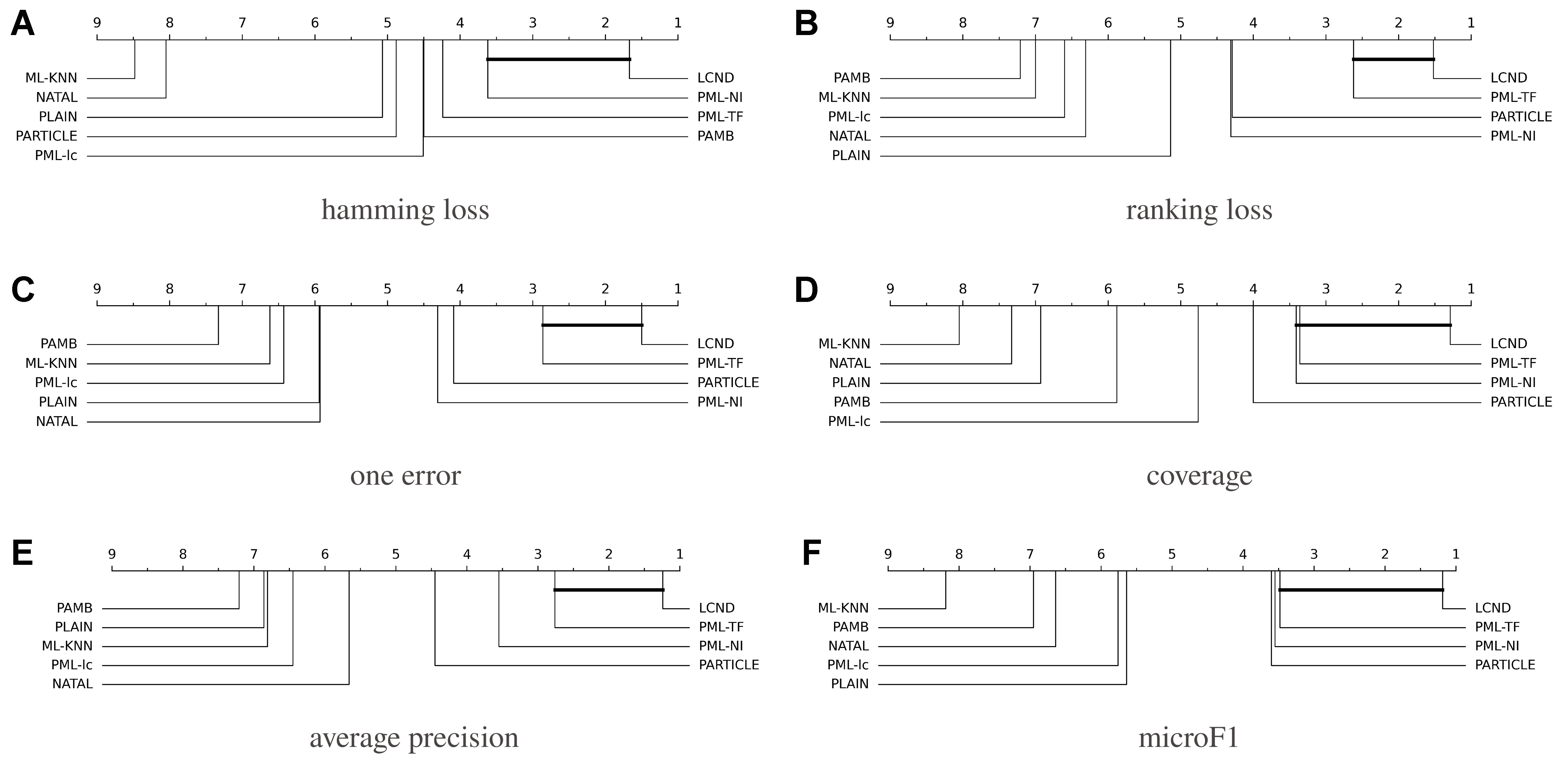
Figure 1. LCND compared with eight algorithms using Bonferroni-Dunn test. If not linked on CD diagram, performance differs significantly (CD = 2.302, 0.05 significance). LCND: Label co-occurrence guided nonlinear disambiguation for partial multi-label learning; CD: critical difference.
From Figure 1, we can observe that:
• LCND achieves the best average ranking across all evaluation metrics. As shown in Figure 1, LCND consistently occupies the rightmost position in the CD diagram for all six metrics, including Hamming loss, Ranking loss, One error, Coverage, Average precision, and microF1. This indicates that LCND outperforms the seven competing algorithms in both error-based and accuracy-based evaluations, demonstrating strong robustness and generalizability.
• LCND is statistically significantly superior to most baseline methods. With a CD threshold of CD = 2.302 at the 0.05 significance level, algorithms that are not connected by a horizontal bar are considered significantly different. LCND is not comparable to the majority of the competing methods (e.g., ML-KNN, PML-lc, PARTICLE, NATAL, PLAIN, PML-TF) on most metrics, confirming that its performance advantage is statistically significant.
• The performance improvement of LCND is most pronounced on ranking-oriented metrics. The gap between LCND and the competing methods is particularly large for Ranking loss and Average precision. This demonstrates that the weighted Jaccard label affinity and nonlinear kernel mapping effectively capture fine-grained label semantics, enabling LCND to better distinguish ground-truth labels from noisy candidates during label ranking.
• LCND achieves a notably better average rank than the recent transformer-based method PML-TF, especially on ranking-oriented metrics, confirming the advantage of explicit nonlinear kernel modeling over implicit deep feature extraction in PML tasks.
4.4. Ablation study
To assess the contribution of key model components, we conduct an ablation study in which we systematically remove these components to observe the resulting changes in performance. The specific configurations for this ablation analysis are outlined below:
• To validate the effectiveness of the nonlinear component P in our model, we perform an ablation analysis by removing this component and evaluating the subsequent performance changes. Specifically, we remove the module g(P)
We refer to this method as LCND-NOK and solve the optimization problem using the ALM method.
• To demonstrate the impact of label affinity, we remove the term α||Z○H||12, which is a constraint in LCND, resulting in a modified method called LCND-NOH.
• To assess the combined influence of the nonlinear component and label affinity, we exclude the label affinity component from the formulation in Equation (36), yielding a variant of the method termed LCND-NOKH.
Figure 2 presents the comparative experimental results of three methods on the music_style, Birds_3, and Medical_3 datasets, where average precision is shown as one minus the average precision (i.e., 1 - Average Precision). Key observations are as follows:
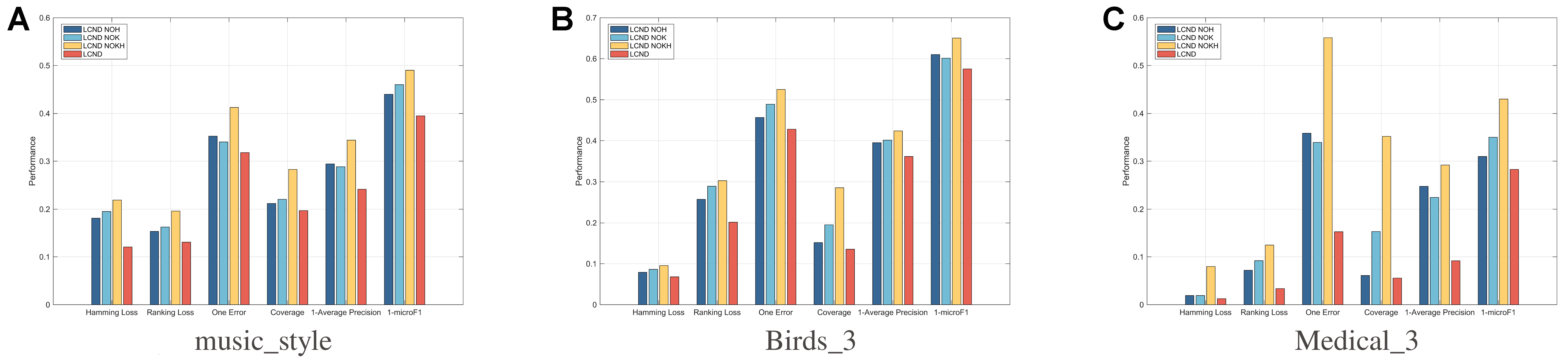
Figure 2. Performance of LCND-NOH, LCND-NOK, LCND-NOKH and LCND. LCND: Label co-occurrence guided nonlinear disambiguation for partial multi-label learning.
• The LCND model outperforms the other methods on all datasets and most metrics, particularly in reducing One Error and improving 1 - Average Precision. The LCND-NOKH model, which lacks both the nonlinear component and label affinity, underperforms compared to LCND-NOK and LCND-NOH. This indicates that jointly modeling label correlations and nonlinear feature structures is essential for achieving optimal performance.
• LCND-NOK performs well on some metrics by modeling features in linear subspaces, but it does not outperform the full model. On the Medical_3 dataset, where the feature dimension is larger than the number of instances (d > n), the need to handle nonlinear problems becomes evident. These results confirm that nonlinear feature induction and label relationships improve training. Our ablation study demonstrates the superior performance and reliability of the complete model.
4.5. Comparison of different kernel functions
To validate the effectiveness and generality of different kernel functions, this section presents comparative experiments using the polynomial, Sigmoid, arctan, and Gaussian kernels on both real-world and synthetic datasets. The results are summarized in Figure 3.
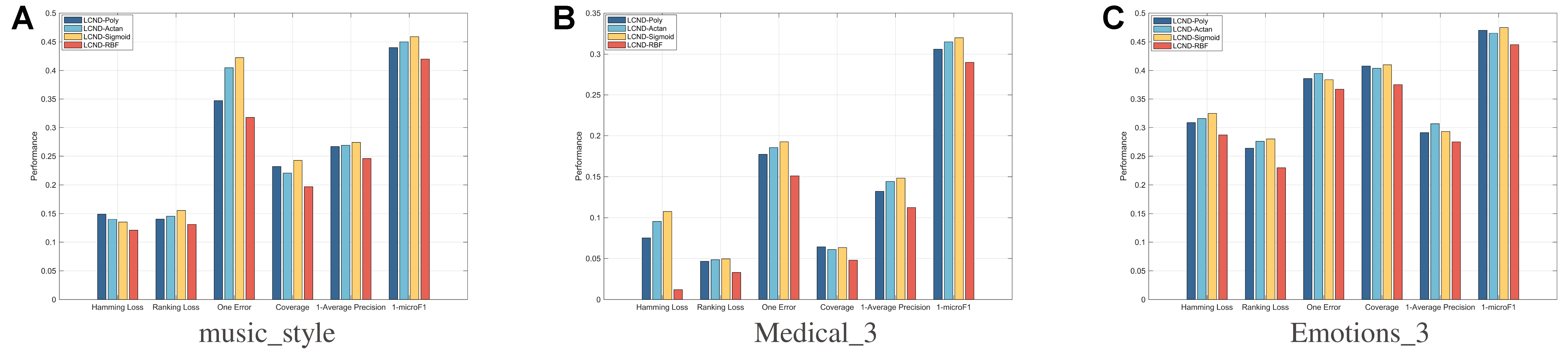
Figure 3. The comparative results of different kernel functions.
As shown in Figure 3, the Gaussian kernel function significantly outperforms all other kernels across all six performance metrics. This superiority stems from the inherent mechanism of the Gaussian kernel: it embeds sample data into an infinite-dimensional RKHS via implicit feature mapping. This property theoretically enables the Gaussian kernel to approximate arbitrarily complex nonlinear decision boundaries, demonstrating exceptional versatility in addressing nonlinear classification problems.
4.6. Comparison of different label functions
To rigorously verify the effectiveness of the proposed weighted Jaccard distance, we conducted additional ablation experiments comparing three variants of label similarity metrics:
1. LCND-H: LCND using the standard Jaccard similarity (i.e., with equal label weights).
2. LCND-CH: LCND using the cosine similarity between label vectors.
The experiments were performed on three representative datasets with distinct characteristics: music_emotion, Medical_3, and Birds_2. The results are shown in Figure 4, from which we make the following observations:
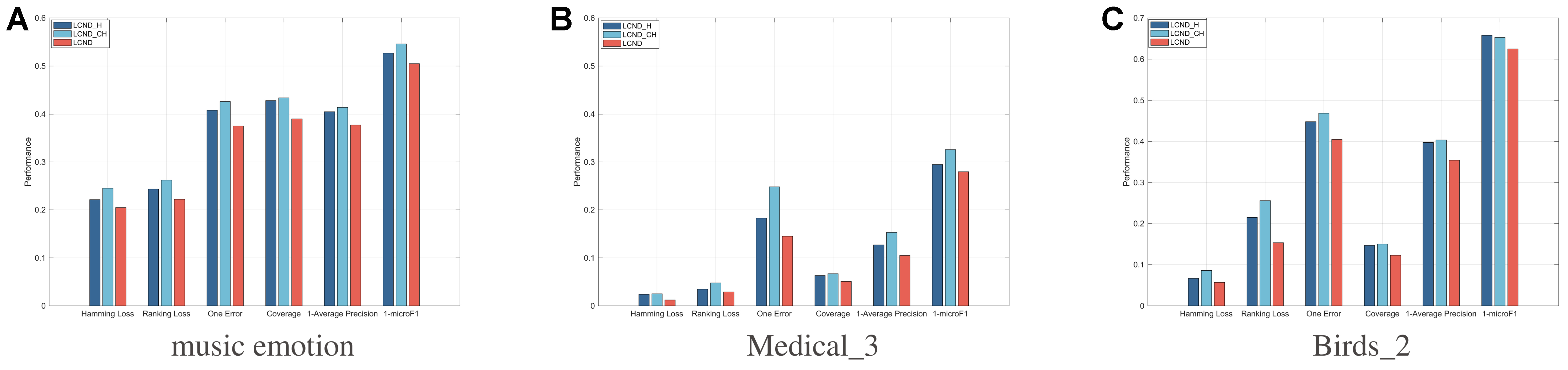
Figure 4. Performance of LCND-H, LCND-CH and LCND. LCND: Label co-occurrence guided nonlinear disambiguation for partial multi-label learning.
1. The weighted Jaccard distance consistently outperforms the standard Jaccard distance. On all three datasets, LCND achieves significantly higher average precision than LCND-H. This improvement arises because the standard Jaccard distance treats all labels equally and cannot distinguish frequent labels from rare, specific, or noisy ones. In contrast, the proposed weighting scheme adaptively enhances the contribution of informative labels while suppressing the influence of noisy or trivial labels.
2. The weighted Jaccard distance also outperforms the cosine similarity. LCND-CH yields the lowest average precision across all datasets. Cosine similarity computed directly on binary label vectors is highly sensitive to the sparsity and label noise in the candidate label sets of PML. In comparison, the weighted Jaccard distance incorporates global label statistics (i.e., label frequency and co-occurrence) and is more robust to random label noise.
These findings demonstrate that the proposed weighted Jaccard distance is a critical component for robust label disambiguation in PML. The weighting scheme effectively leverages global label statistics to mitigate the adverse effects of label noise and sparsity, achieving consistent and significant performance improvements over both the standard Jaccard distance and the cosine similarity.
4.7. Parameter analysis
Within the scope of this study, we consider four regularization parameters: α, β, γ, and λ. These parameters are selected from the interval [10-3, 103] using a grid search strategy. To investigate its impact, we present experimental results of the LCND classifier by adjusting one parameter at a time while keeping the other three fixed. The data in Figures 5 and 6 indicate that the overall trends of α and γ remain stable across different datasets. The λ parameter is also stable except for the extremely small value of 10-3. The β parameter first increases and then decreases as its value increases, with the optimal parameter range consistently falling between 1 and 10 across all datasets.
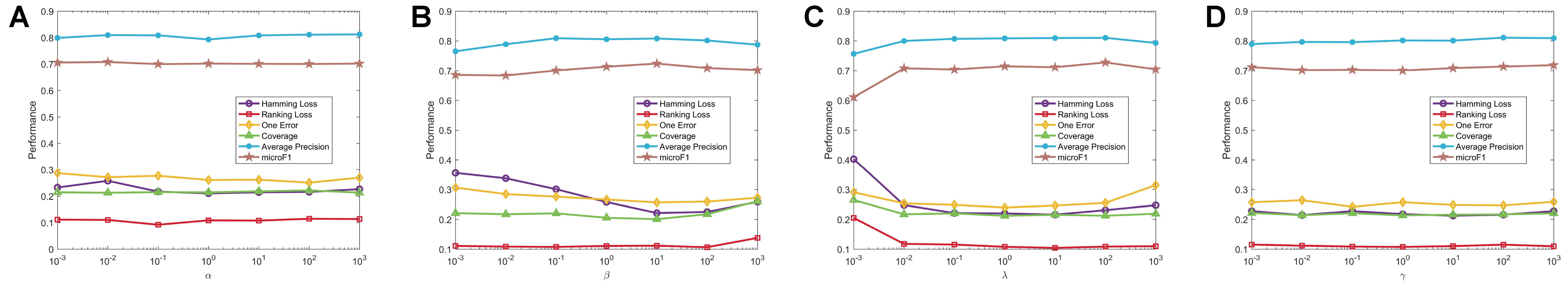
Figure 5. The performance of LCND on the mirflickr dataset across a range of trade-off parameter values. LCND: Label co-occurrence guided nonlinear disambiguation for partial multi-label learning.
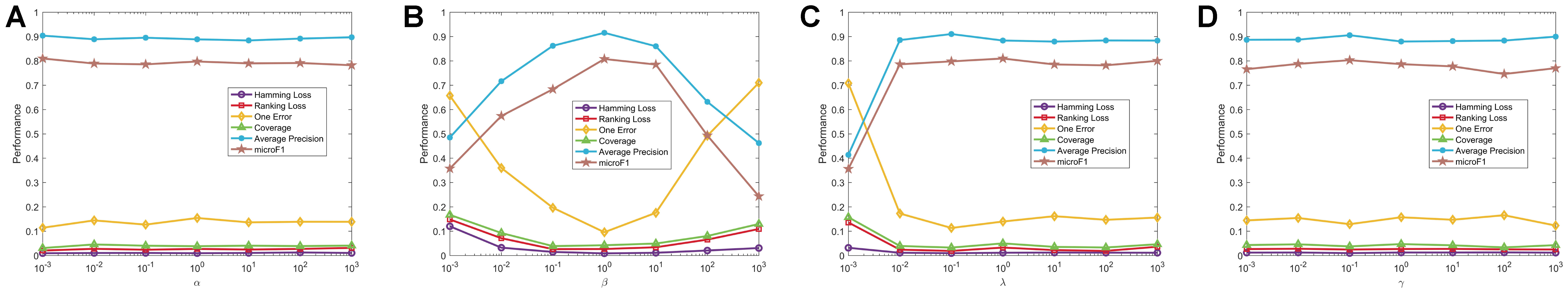
Figure 6. The performance of LCND on the Medical_1 dataset across a range of trade-off parameter values. LCND: Label co-occurrence guided nonlinear disambiguation for partial multi-label learning.
4.8. Computational complexity
In the context of the LCND algorithm, TLCND denotes the total number of iterations required. It is not necessary to compute the inverse (XVVTXT + 2βId)-1 at every iteration; thus, computing W according to Equation (18) incurs a complexity of
We note that the label affinity matrix H constructed via the weighted Jaccard distance is highly sparse in practice. Because the candidate label sets of most instance pairs have little or no overlap, the vast majority of entries in H are either exactly zero or negligibly small. In our implementation, H can be stored in a sparse matrix format. This sparsity significantly reduces the computational cost of the element-wise product Z○H and the associated ℓ1 penalty. Moreover, the sparse structure of H naturally encourages sparsity in the learned instance affinity matrix Z, which in turn enables the use of scalable sparse linear algebra routines and iterative solvers, thereby avoiding full n × n matrix inversions. This sparsity-driven strategy provides a practical and effective way to extend LCND to large-scale datasets while fully preserving its nonlinear modeling capability.
5. CONCLUSION
This paper proposes LCND, a novel framework designed to address nonlinear, partial, MLL problems. By leveraging kernel LRR, it effectively captures nonlinear data associations often overlooked by conventional linear methods, while integrating a weighted Jaccard distance to quantify label correlations and enhance label denoising. Empirical results show that LCND outperforms traditional approaches, highlighting the importance of modeling nonlinear data structures and label interconnections. This work offers a new perspective for tackling complex PML tasks. Future work will focus on extending LCND to a broader range of applications.
DECLARATIONS
Authors’ contributions
Made substantial contributions to conception and design of the study and performed data analysis and interpretation: Song, Y.; Qi, F.; Feng, J.; Li, Z.
Performed data acquisition, as well as provided administrative, technical, and material support: Huang, L.; Bu, Q.; Lu, W.; Fan, J.
Availability of data and materials
The Music Emotion and Music Style datasets used in this study are publicly available in the PALM Lab Partial Multi-label Learning Dataset Repository at https://palm.seu.edu.cn/zhangml/Resources.htm[44]. The Mirflickr data used in this study are publicly available in the PALM Lab Partial Multi-label Learning Dataset Repository at https://palm.seu.edu.cn/zhangml/Resources.htm[60].
The image data used in this study are publicly available in the PALM Lab Partial Multi-label Learning Dataset Repository at https://palm.seu.edu.cn/zhangml/Resources.htm[9].
The BibTex data presented in this study are available in the Mulan Multi-label Learning Dataset Repository at https://mulan.sourceforge.net/datasets-mlc.html[61].
The birds’ data presented in this study are available in Mulan Multi-label Learning Dataset Repository at https://mulan.sourceforge.net/datasets-mlc.html[62].
The emotions data presented in this study are available in Mulan Multi-label Learning Dataset Repository at https://mulan.sourceforge.net/datasets-mlc.html[63].
The medical data presented in this study are available in Mulan Multi-label Learning Dataset Repository at https://mulan.sourceforge.net/datasets-mlc.html[64].
The scene data presented in this study are available in Mulan Multi-label Learning Dataset Repository at https://mulan.sourceforge.net/datasets-mlc.html[8].
AI and AI-assisted tools statement
Not applicable.
Financial support and sponsorship
This research was supported by the National Natural Science Foundation of China (under Project No. 62401309), the Natural Science Foundation of Shandong Province (under Project No. ZR2024QF119), the Qingdao Natural Science Foundation Project (under Project No. 24-4-4-zrjj-89-jch), the China Postdoctoral Science Foundation (under Project No. 2025M771692), the Open Fund Project of Key Laboratory of Computing Power Internet and Information Security, Ministry of Education (under Project No. 2024PY030), and the National Natural Science Foundation of China (under Project No. 62376130).
Conflicts of interest
All authors declared that there are no conflicts of interest.
Ethical approval and consent to participate
Not applicable.
Consent for publication
Not applicable.
Copyright
© The Author(s) 2026.
Supplementary Materials
REFERENCES
1. Zhang, M. L.; Zhou, Z. H. A review on multi-label learning algorithms. IEEE. Trans. Knowl. Data. Eng. 2014, 26, 1819-37.
2. Qian, W.; Xiong, Y.; Ding, W.; Huang, J.; Vong, C. M. Label correlations-based multi-label feature selection with label enhancement. Eng. Appl. Artif. Intell. 2024, 127, 107310.
3. Fu, D.; Zhong, H.; Zhang, X.; et al. Graph relationship-driven label coded mapping and compensation for multi-label textile fiber recognition. Eng. Appl. Artif. Intell. 2024, 133, 108484.
4. Zhang, P.; Gao, W.; Hu, J.; Li, Y. A conditional-weight joint relevance metric for feature relevancy term. Eng. Appl. Artif. Intell. 2021, 106, 104481.
5. Han, Q.; Hu, L.; Gao, W. Feature relevance and redundancy coefficients for multi-view multi-label feature selection. Inf. Sci. 2024, 652, 119747.
6. Mu, J.; Chen, Y.; Sun, W.; Wan, Z.; Wang, S.; Tao, T. Classifier enhancement based on credible sample selection for partial multi-label learning. Appl. Intell. 2025, 55, 1006.
7. Xie, M. K.; Huang, S. J. Partial multi-label learning. Proc. AAAI. Conf. Artif. Intell. 2018, 32.
8. Boutell, M. R.; Luo, J.; Shen, X.; Brown, C. M. Learning multi-label scene classification. Pattern. Recogn. 2004, 37, 1757-71.
9. Zhang, M. L.; Zhou, Z. H. ML-KNN: a lazy learning approach to multi-label learning. Pattern. Recogn. 2007, 40, 2038-48.
10. Chen, Y. N.; Lin, H. T. Feature-aware label space dimension reduction for multi-label classification. 2012. https://proceedings.neurips.cc/paper/2012/file/d4c2e4a3297fe25a71d030b67eb83bfc-Paper.pdf. (accessed 2026-06-26).
11. Zhang, J.; Jiang, X.; Tian, N.; Wu, M. Label noise correction for crowdsourcing using dynamic resampling. Eng. Appl. Artif. Intell. 2024, 133, 108439.
12. Sun, F.; Xie, M. K.; Huang, S. J. A deep model for partial multi-label image classification with curriculum-based disambiguation. Mach. Intell. Res. 2024, 21, 801-14.
13. Sun, L.; Feng, S.; Wang, T.; Lang, C.; Jin, Y. Partial multi-label learning by low-rank and sparse decomposition. Proc. AAAI. Conf. Artif. Intell. 2019, 33, 5016-23.
14. Sun, L.; Feng, S.; Liu, J.; Lyu, G.; Lang, C. Global-local label correlation for partial multi-label learning. IEEE. Trans. Multimedia. 2021, 24, 581-93.
15. Xie, M. K.; Huang, S. J. Partial multi-label learning with noisy label identification. IEEE. Trans. Pattern. Anal. Mach. Intell. 2022, 44, 3676-87.
16. Liu, B. Q.; Jia, B. B.; Zhang, M. L. Towards enabling binary decomposition for partial multi-label learning. IEEE. Trans. Pattern. Anal. Mach. Intell. 2023, 45, 13203-17.
17. Zhang, P.; Gao, W.; Hu, J.; Li, Y. Multi-label feature selection based on high-order label correlation assumption. Entropy 2020, 22, 797.
18. Liu, G.; Lin, Z.; Yu, Y. Robust subspace segmentation by low-rank representation. In Proceedings of the 27th International Conference on Machine Learning (ICML-10). Omnipress: 2010; pp. 663-70.
19. Jiang, W.; Liu, J.; Qi, H.; Dai, Q. Robust subspace segmentation via nonconvex low rank representation. Inf. Sci. 2016, 340-1, 144-58.
20. Xiao, S.; Tan, M.; Xu, D.; Dong, Z. Y. Robust kernel low-rank representation. IEEE. Trans. Neural. Netw. Learn. Syst. 2016, 27, 2268-81.
21. Li, Z.; Liu, J.; Tang, J.; Lu, H. Robust structured subspace learning for data representation. IEEE. Trans. Pattern. Anal. Mach. Intell. 2015, 37, 2085-98.
22. Tanfous, A. B.; Drira, H.; Amor, B. B. Sparse coding of shape trajectories for facial expression and action recognition. IEEE. Trans. Pattern. Anal. Mach. Intell. 2020, 42, 2594-607.
23. Roweis, S. T.; Saul, L. K. Nonlinear dimensionality reduction by locally linear embedding. Science 2000, 290, 2323-6.
24. Abdolali, M.; Gillis, N. Beyond linear subspace clustering: a comparative study of nonlinear manifold clustering algorithms. Comput. Sci. Rev. 2021, 42, 100435.
25. Li, H.; Fang, M.; Li, X.; Chen, B. An adaptive class prototype generation framework for partial label learning. Eng. Appl. Artif. Intell. 2024, 133, 108178.
26. Li, W.; Fan, L.; Shao, S.; Song, A. Generalized contrastive partial label learning for cross-subject EEG-based emotion recognition. IEEE. Trans. Instrum. Meas. 2024, 73, 1-11.
27. Fan, J.; Yu, Y.; Wang, Z. Partial label learning with competitive learning graph neural network. Eng. Appl. Artif. Intell. 2022, 111, 104779.
28. Feng, L.; An, B. Partial label learning by semantic difference maximization. In Proceedings of the Twenty-Eighth International Joint Conference on Artificial Intelligence. 2019; pp. 2294-300.
29. Liu, L. P.; Dietterich, T. G. A conditional multinomial mixture model for superset label learning. In Proceedings of the 26th International Conference on Neural Information Processing Systems. Curran Associates Inc.: 2012; pp. 548-56.
30. Cour, T.; Sapp, B.; Taskar, B. Learning from partial labels. J. Mach. Learn. Res. 2011, 12, 1501-36. https://jmlr.csail.mit.edu/papers/v12/cour11a.html. (accessed 2026-06-26).
31. Gong, C.; Liu, T.; Tang, Y.; Yang, J.; Yang, J.; Tao, D. A regularization approach for instance-based superset label learning. IEEE. Trans. Cybern. 2018, 48, 967-78.
32. Gong, X.; Yang, J.; Yuan, D.; Bao, W. Generalized large margin kNN for partial label learning. IEEE. Trans. Multimedia. 2021, 24, 1055-66.
33. Sun, K.; Min, Z.; Wang, J. PP-PLL: probability propagation for partial label learning. In Machine Learning and Knowledge Discovery in Databases: European Conference, ECML PKDD 2019, Würzburg, Germany, September 16-20, 2019; Springer; 2020; pp. 123-37.
34. Wang, W.; Zhang, M. L. Partial label learning with discrimination augmentation. In Proceedings of the 28th ACM SIGKDD Conference on Knowledge Discovery and Data Mining. Association for Computing Machinery: 2022; pp. 1920-8.
35. Lyu, G.; Feng, S.; Huang, W.; Dai, G.; Zhang, H.; Chen, B. Partial label learning via low-rank representation and label propagation. Soft. Comput. 2020, 24, 5165-76.
36. Wang, S.; Xia, M.; Wang, Z.; Lyu, G.; Feng, S. Partial label learning with noisy side information. Appl. Intell. 2022, 52, 12382-96.
37. Gong, B.; Zhou, R.; Jing, L. Convolutional attention-based contrastive learning for partial label learning. Appl. Intell. 2025, 55, 868.
38. Li, H.; Wan, Z.; Vong, C. M. Multi-kernel partial label learning using graph contrast disambiguation. Appl. Intell. 2024, 54, 9760-82.
39. Zhang, M. L.; Yu, F.; Tang, C. Z. Disambiguation-free partial label learning. IEEE. Trans. Knowl. Data. Eng. 2017, 29, 2155-67.
40. Lyu, G.; Feng, S.; Wang, T.; Lang, C.; Li, Y. GM-PLL: Graph matching based partial label learning. IEEE. Trans. Knowl. Data. Eng. 2021, 33, 521-35.
41. Feng, L.; Lv, J.; Han, B.; et al. Provably consistent partial-label learning. arXiv 2020, arXiv:2007.08929. Available online: https://doi.org/10.48550/arXiv.2007.08929. (accessed 2026-06-26).
42. Liu, L. P.; Dietterich, T. G. Learnability of the superset label learning problem. In International Conference on Machine Learning. 2014. https://api.semanticscholar.org/CorpusID:17882853. (accessed 2026-06-26).
43. Xu, N.; Liu, B.; Lv, J.; Qiao, C.; Geng, X. Progressive purification for instance-dependent partial label learning. In Proceedings of the 40th International Conference on Machine Learning. PMLR: 2023; pp. 38551-65. https://proceedings.mlr.press/v202/xu23l.html. (accessed 2026-06-26).
44. Zhang, M. L.; Fang, J. P. Partial multi-label learning via credible label elicitation. IEEE. Trans. Pattern. Anal. Mach. Intell. 2021, 43, 3587-99.
45. Wang, H.; Liu, W.; Zhao, Y.; Zhang, C.; Hu, T.; Chen, G. Discriminative and correlative partial multi-label learning. In Proceedings of the Twenty-Eighth International Joint Conference on Artificial Intelligence. 2019; pp. 3691-7.
46. Yu, G.; Chen, X.; Domeniconi, C.; Wang, J.; Li, Z.; Zhang, Z. Feature-induced partial multi-label learning. In 2018 IEEE international conference on data mining (ICDM), Singapore, Nov 17-20, 2018. IEEE; 2018. pp. 1398-403.
47. Gong, X.; Yuan, D.; Bao, W. Understanding partial multi-label learning via mutual information. In 35th Conference on Neural Information Processing Systems (NeurIPS 2021). 2021; pp. 4147-56. https://proceedings.neurips.cc/paper/2021/file/217c0e01c1828e7279051f1b6675745d-Paper.pdf. (accessed 2026-06-26).
48. Wu, J. H.; Wu, X.; Chen, Q. G.; Hu, Y.; Zhang, M. L. Feature-induced manifold disambiguation for multi-view partial multi-label learning. In Proceedings of the 26th ACM SIGKDD International Conference on Knowledge Discovery & Data Mining. Association for Computing Machinery: 2020; pp. 557-65.
49. Hao, P.; Hu, L.; Gao, W. Partial multi-label feature selection via subspace optimization. Inf. Sci. 2023, 648, 119556.
50. Hang, J. Y.; Zhang, M. L. Partial multi-label learning with probabilistic graphical disambiguation. In 37th Conference on Neural Information Processing Systems (NeurIPS 2023). 2023; pp. 1339-51. https://proceedings.neurips.cc/paper_files/paper/2023/file/04e05ba5cbc36044f6499d1edf15247e-Paper-Conference.pdf. (accessed 2026-06-26).
51. Wang, Z.; Liu, F.; Han, M.; Tang, H.; Wan, B. PML-ED: a method of partial multi-label learning by using encoder-decoder framework and exploring label correlation. Inf. Sci. 2024, 661, 120165.
52. Li, Z.; Huang, L.; Gu, T.; Bu, Q.; Qi, F.; Fan, J. Partial multi-label learning via K-means graph transformer. Knowl. Based. Syst. 2025, 325, 114017.
53. Qi, F.; Huang, L.; Feng, J.; et al. Nonlinear characteristic-driven partial multi-label learning. In Advances in Knowledge Discovery and Data Mining. Springer Nature Singapore: 2026; pp. 442-54.
54. Yang, J.; Ma, J.; Win, K. T.; Gao, J.; Yang, Z. Low-rank and sparse representation based learning for cancer survivability prediction. Inf. Sci. 2022, 582, 573-92.
55. Fan, J.; Yu, Y.; Wang, Z. Addressing label ambiguity imbalance in candidate labels: measures and disambiguation algorithm. Inf. Sci. 2022, 612, 1-19.
56. Zhang, P.; Gao, W. Feature relevance term variation for multi-label feature selection. Appl. Intell. 2021, 51, 5095-110.
57. Gao, W.; Hu, J.; Li, Y.; Zhang, P. Feature redundancy based on interaction information for multi-label feature selection. IEEE. Access. 2020, 8, 146050-64.
58. Auricchio, G.; Brigati, G.; Giudici, P.; Toscani, G. Multivariate Gini-type discrepancies. Math. Models. Methods. Appl. Sci. 2025, 35, 1267-96.
59. Lin, Z.; Liu, R.; Su, Z. Linearized alternating direction method with adaptive penalty for low-rank representation. In Proceedings of the 25th International Conference on Neural Information Processing Systems. Curran Associates Inc.: 2011; pp. 612-20.
60. Huiskes, M. J.; Lew, M. S. The MIR flickr retrieval evaluation. In Proceedings of the 1st ACM International Conference on Multimedia Information Retrieval. Association for Computing Machinery: 2008; pp. 39-43.
61. Katakis, I.; Tsoumakas, G.; Vlahavas, I. Multilabel text classification for automated tag suggestion. 2008. https://api.semanticscholar.org/CorpusID:15676013. (accessed 2026-06-26).
62. Briggs, F.; Huang, Y.; Raich, R.; et al. The 9th annual MLSP competition: new methods for acoustic classification of multiple simultaneous bird species in a noisy environment. In 2013 IEEE international workshop on machine learning for signal processing (MLSP), Southampton, UK, Sep 22-25, 2013. IEEE; 2013. p. 1-8.
63. Trohidis, K.; Tsoumakas, G.; Kalliris, G.; Vlahavas, I. Multi-label classification of music into emotions. 2008; pp. 325-30. https://www.researchgate.net/publication/288623967_Multilabel_classification_of_music_into_emotions. (accessed 2026-06-26).
64. Pestian, J. P.; Brew, C.; Matykiewicz, P.; et al. A shared task involving multi-label classification of clinical free text. In Biological, translational, and clinical language processing, Prague, Czech Republic, 2007. Association for Computational Linguistics: 2007; pp. 97-104. https://aclanthology.org/W07-1013/. (accessed 2026-06-26).
65. Lyu, G.; Feng, S.; Li, Y. Noisy label tolerance: a new perspective of partial multi-label learning. Inf. Sci. 2021, 543, 454-66.
66. Wang, H.; Yang, S.; Lyu, G.; et al. Deep partial multi-label learning with graph disambiguation. arXiv 2023, arXiv:2305.05882. Available online: https://doi.org/10.48550/arXiv.2305.05882. (accessed 2026-06-26).
67. Fan, J.; Li, J.; Lu, W.; Huang, L. Partial multi-label learning via transformer to discover discriminative label embeddings. Neurocomputing 2026, 684, 133518.
68. Demšar, J. Statistical comparisons of classifiers over multiple data sets. J. Mach. Learn. Res. 2006, 7, 1-30. https://www.jmlr.org/papers/volume7/demsar06a/demsar06a.pdf. (accessed 2026-06-26).
Cite This Article
How to Cite
Download Citation
Export Citation File:
Type of Import
Tips on Downloading Citation
Citation Manager File Format
Type of Import
Direct Import: When the Direct Import option is selected (the default state), a dialogue box will give you the option to Save or Open the downloaded citation data. Choosing Open will either launch your citation manager or give you a choice of applications with which to use the metadata. The Save option saves the file locally for later use.
Indirect Import: When the Indirect Import option is selected, the metadata is displayed and may be copied and pasted as needed.
About This Article
Copyright

Data & Comments
Data
0


Comments
Comments must be written in English. Spam, offensive content, impersonation, and private information will not be permitted. If any comment is reported and identified as inappropriate content by OAE staff, the comment will be removed without notice. If you have any queries or need any help, please contact us at [email protected].