


Subterranean roadway deformation detection based on LiDAR scanning and fusion filtering
 0
0 Abstract
Underground engineering is becoming increasingly important in modern urban construction and mine development. However, the shape of underground roadways may deform elastically or plastically due to geological conditions and accident loads, a phenomenon that cannot be ignored. Therefore, this paper proposes a roadway deformation detection method based on laser scanning. First, the working principle of the point cloud denoising and downsampling method is explained. To overcome the limitations of this method, the paper presents a point cloud denoising approach that combines statistical and median filtering. Additionally, it introduces a voxelised grid-downsampling technique based on density constraints and the centre of gravity. Next, the bidirectional projection method is used to determine the roadway’s central axis. Then, CloudCompare point cloud processing software is used to segment the point cloud, extract the roadway section, and fit a contour curve. Finally, the methods for extracting roadway deformation from processed point cloud data and for detecting and analysing it are introduced. Experiments on roadway deformation detection are conducted on an inspection robot experimental platform to verify the feasibility of the overall scheme. Experimental results indicate that the measurement error of light detection and ranging scanning for tunnel contour is less than 2 mm.
Keywords
1. INTRODUCTION
A subterranean roadway or tunnel is typically a long, narrow, enclosed space that provides an unfavourable working environment[1]. The stability of the roadway is important for coal mining, transportation, and worker safety. Deformation of a coal mine roadway refers to changes in its shape caused by factors such as ground conditions, surrounding rock pressure, and vibrations from transport vehicles during mining[2]. Cracks in the roadway can seriously affect its reliability and safety, especially in deep roadways[3]. Therefore, improving the accuracy of point cloud data measurements based on distance is important[4,5].
Currently, tunnel deformation monitoring primarily relies on stress sensors, fibre-optic grating sensors[6], laser ranging[7], visual measurements[8,9], interferometric synthetic aperture radar (InSAR)[10], and 3D light detection and ranging (LiDAR) scanning[11]. Among them, roadway deformation monitoring methods based on stress sensors and fibre-optic grating sensors are contact-based; however, they can only monitor deformations at discrete points, with low automation, limited work efficiency, and low data density. The accuracy of visual measurement is easily affected by environmental factors such as underground illumination, dust, and vibration. Laser ranging and scanning can accurately identify the roadway surface deformations, such as displacement, convergence, and peeling, and the detection accuracy can reach centimetre level. Ji et al. accurately position and precisely segment the rings and block a shield tunnel in three-dimensional (3D) point cloud data by detecting the shape and positional characteristics of the tunnel support bolts’ laser point clouds[12,13]. Singh et al. combined a multi-scale Canopy classifier and a random sample consensus (RANSAC) shape-detection algorithm to propose a method for identifying roadway roof bolts using 3D point cloud data captured by a mobile laser scanner[14]. This method provides robust bolt identification. Maes et al. identify small changes in tunnel response based on linear principal component analysis; however, this method cannot distinguish the nature of the changes in tunnel response[15]. Luo and Lin proposed a new method to automatically measure the geometric shape of a ramp at the network level using an inertial measurement unit (IMU) and a 3D LiDAR system[16]. This method improves the robustness of slope geometric measurement. Morago et al. proposed a discontinuous rock measurement method based on the fusion of vision and LiDAR scanning, achieving a more balanced measurement of rock cracks[17]. Yasuda and Ying estimate tunnel deformation using the difference in the Fourier series representation of the tunnel profile before and after deformation, and improve stress estimation accuracy by using higher-order Fourier series terms[4]. Hu et al. extracted deformation information from measuring points on the tunnel lining surface using an improved Kriging filtering algorithm[18]. They then verified tunnel deformation monitoring based on 3D laser scanning technology through field monitoring experiments. Yang and Xu used the reflection intensity to extract tunnel structural cracks, thereby reducing deviations in the automatic identification and extraction process[3]. Cui et al. proposed a wavelet filtering algorithm to filter point clouds on tunnel cross sections, which was used to detect dislocations in tunnel segments[19].
This paper presents a method for acquiring point cloud data of roadways using laser scanning technology. First, the obtained point cloud data are preprocessed, and useless noise points are eliminated through point cloud filtering. Then, a downsampling algorithm sparsifies the point cloud data to improve processing efficiency while retaining the geometric characteristics of the roadway outline. Next, the point set of the roadway central axis is extracted using the bidirectional projection method. The RANSAC algorithm is then used to fit the central axis for segmentation and extraction of the roadway section. Finally, point cloud post-processing software extracts and fits the roadway profile. Deformation of the roadway is analysed based on the profile information.
2. INFORMATION ACQUISITION OF ROADWAY POINT CLOUD
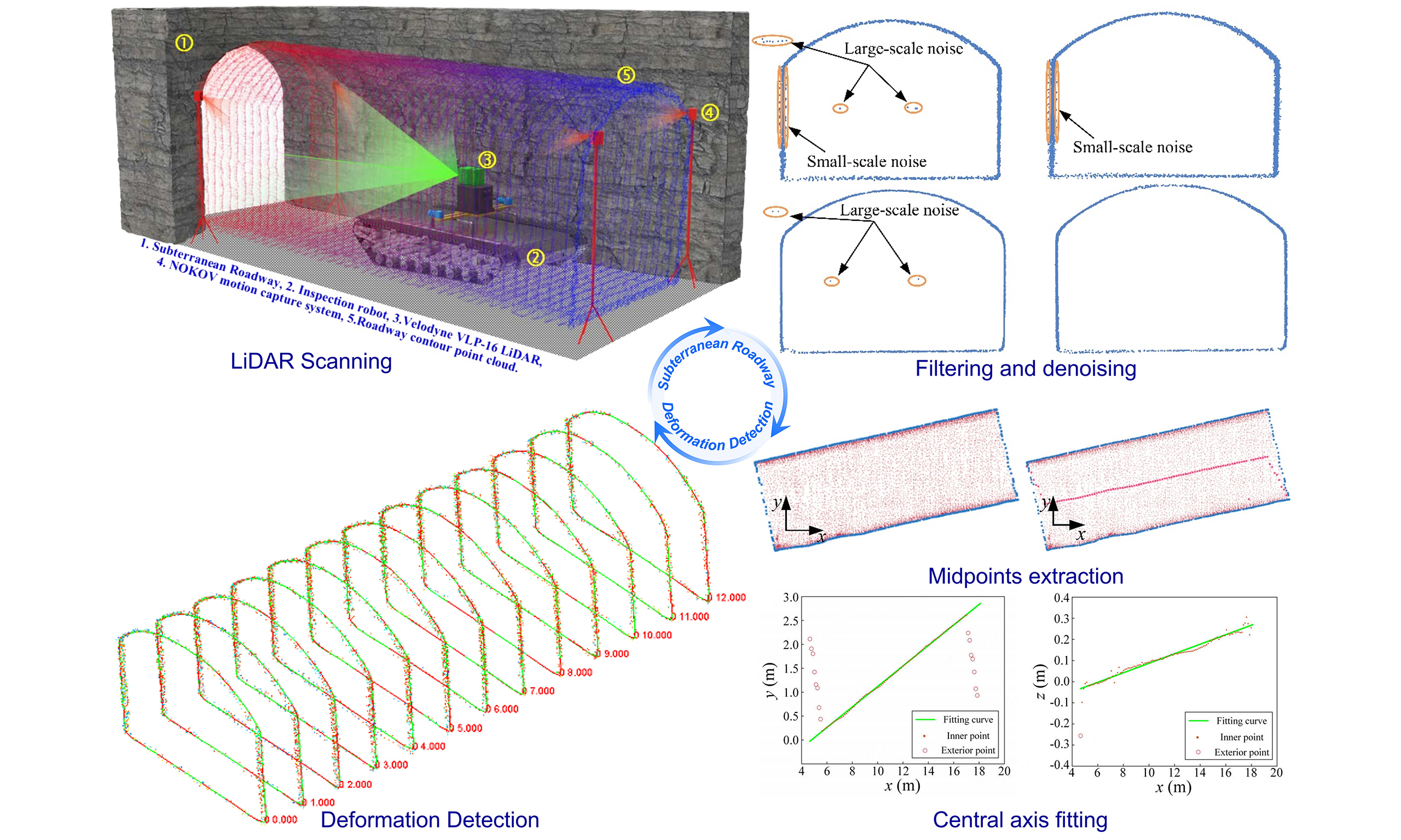
The acquisition of 3D point cloud data uses the principle of laser ranging to record the 3D coordinates, reflectivity, and texture of environmental features. These features are then saved as point cloud data. The present paper employs a mobile inspection robot that is equipped with a VLP-16 LIDAR sensor (by Velodyne Co., Ltd., America) as its experimental platform. The robot employs mobile laser scanning technology to obtain point cloud data of the roadway environment and extract roadway deformation. As illustrated in Figure 1, the experimental setup for the coal mine roadway inspection robot and the process of acquiring roadway point cloud data are shown. The inspection robot, equipped with a 3D LiDAR, is deployed in the coal mine roadway. The movement of the robot through the environment enables the LiDAR to scan the entire roadway and collect point cloud data. The LiDAR point cloud data is then processed to extract the roadway contour information for the analysis of its deformation state.
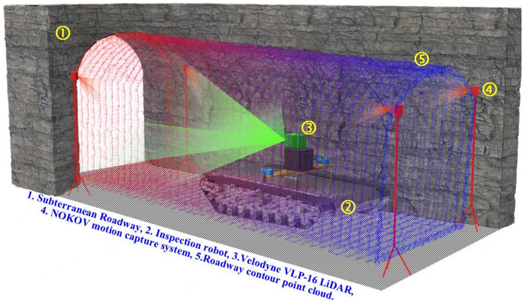
Figure 1. Schematic diagram of mine roadway point cloud data acquisition. LiDAR: Light detection and ranging.
2.1. Denoising method of LiDAR point cloud
During the acquisition of roadway point cloud data by laser scanning, the original data typically contains noise arising from external factors, including poor environmental conditions, equipment interference, and interference from the surface of the measured object. There are two approaches to point cloud denoising: manual and automatic. Manual denoising entails the elimination of noise points after importing the point cloud files into processing software. The automatic denoising process employs a filtering algorithm that automatically eliminates irrelevant points. Manual denoising of large amounts of laser scanning data is inefficient and can result in the elimination of valid point cloud data. Consequently, the primary function of filtering algorithms is denoising. In the experimental environment of this paper, it is necessary to manually and automatically denoise the original point cloud data due to the proximity of certain non-target objects to the inner wall of the roadway. This ensures the removal of all types of noise. Two categories of noise are evident in point cloud data: large-scale and small-scale. To consider the influence of different point cloud filtering algorithms on the accuracy of the original point cloud data, statistical filtering and median filtering are used to eliminate noise. Statistical filtering is effective at removing large-scale noise but is ineffective at removing small-scale noise at the edge of the point cloud. Conversely, median filtering exhibits the opposite behaviour. Therefore, a combined filtering algorithm using statistical and median filtering is employed to better remove noise from the point cloud data obtained in this paper. The purpose is to meet the requirements of point cloud denoising while maintaining the detailed characteristics of the data before and after denoising, as illustrated in Figure 2.
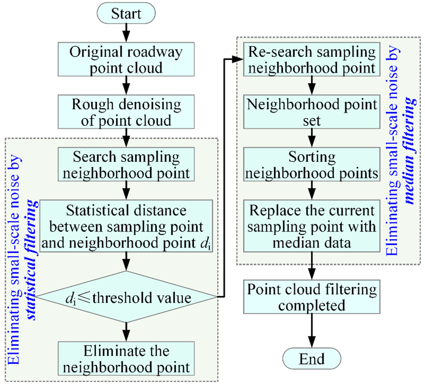
Figure 2. Flowchart of the combined filtering method for denoising.
As shown in Figure 2, the integration of filtering and denoising techniques begins with the manual elimination of invalid data from the original point cloud. Subsequently, a statistical filtering algorithm is employed to eliminate large-scale noise. In conclusion, the implementation of a median filtering algorithm is instrumental in eliminating minor noise and enhancing the smoothness of point cloud data. In order to verify the effectiveness of the combined filtering method, a section of the point cloud with a certain thickness is filtered based on the point cloud data of the simulated roadway shown in Figure 3.
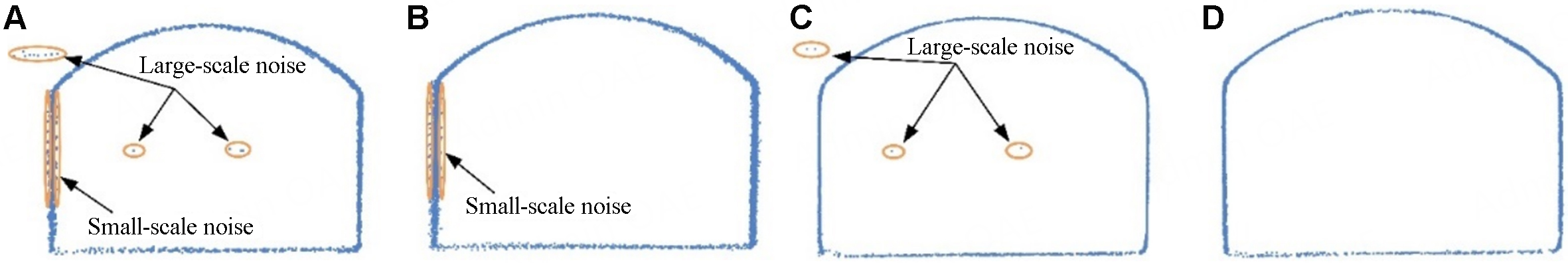
Figure 3. Comparison of point cloud filtering results. (A) Original; (B) Statistical filtering; (C) Median filtering; (D) Combined filtering.
Firstly, as illustrated in Figure 3A, the original point cloud contains both large- and small-scale noise, including outliers and burrs at the edge of the point cloud. As shown in Figure 3B, statistical filtering is an effective method for removing outliers from an original point cloud, consistent with previous research. However, removing mixed points from the edge of the point cloud is ineffective, if not impossible. Thirdly, Figure 3C shows that median filtering is an effective method of removing small-scale noise, including mixed points and burrs from the edge of the point cloud. However, it is not possible to completely eliminate outliers. A comparison of the combined filtering method with the first two filtering methods shows that the former is more effective at removing size and scale noise from the original point cloud. This is achieved using statistical and median filtering. The edge features of the point cloud are shown to be smoother after filtration, as shown in Figure 3D. As shown in the preceding analysis, the combined filtering method is more effective at denoising and conducive to the subsequent processing of point cloud data.
We statistically analysed the information before and after filtering the original point cloud to quantify the denoising effect of the combined filtering, as shown in Table 1. As Table 1 shows, there are fewer outliers in the intercepted cross-section point cloud. Therefore, statistical filtering removes relatively few noise points compared to median filtering and combined denoising methods. Consequently, the processing time is relatively low. Overall, the combined filtering method combines the characteristics of statistical and median filtering, removing both large- and small-scale noise. Combining the two algorithms reduces point cloud processing time to some extent from a program-simplification standpoint, and the resulting performance meets the needs of this paper.
Statistical analysis of point cloud information before and after filtering
| Types of point cloud | Number of points after downsampling | Number of noise points removed | Consumption time/ms |
| Original point cloud | 3,409 | / | / |
| Point cloud after statistical filtering and denoising | 3,379 | 30 | 3.99 |
| Point cloud after median filtering and denoising | 3,166 | 243 | 263.04 |
| Point cloud after combined filtering and denoising | 3,105 | 304 | 225.90 |
2.2. Sparse sampling of LiDAR point cloud
As LiDAR technology advances, the amount of point cloud data obtained through laser scanning is increasing, especially with systems such as the 16-line 3D LiDAR discussed in this paper. Because of the large volume of point cloud data, processing it directly would be inefficient; so downsampling is necessary to simplify the data. Downsampling is a common method for simplifying point clouds. It transforms a high-density point cloud into a moderate-density point cloud, which is more conducive to extracting roadway cross-section contour features and deformation. Two indices are generally used to evaluate the quality of a downsampling algorithm: precision and simplicity. The objective is to minimise the number of point clouds while maintaining the detailed characteristics of the original point clouds. Based on these two performance evaluation indicators, selecting an appropriate algorithm for the actual point cloud downsampling process is crucial. The algorithm should achieve high simplification while minimising the loss of point cloud details. The voxel-based grid downsampling algorithm is simple and efficient, ensuring that the external contour and spatial structure characteristics of the original point cloud remain essentially unchanged. Therefore, to support subsequent point cloud data processing, this paper uses a voxel grid downsampling algorithm to simplify the point cloud. As shown in Figure 4, the voxelised grid downsampling algorithm[20] is a re-quantisation process.

Figure 4. Voxelised grid sampling schematic diagram. (A) Bounding box construction; (B) Voxelisation; (C) Select sampling point.
First, a grid cube is constructed based on the point cloud data, as shown in Figure 4A. Next, the grid cube is divided into smaller cubes via voxelisation [Figure 4B]. Finally, the centre of gravity of each small cube is found for resampling. Figure 4C illustrates the blue points as the original point cloud and the green points as the points after resampling. The centre of gravity of each small cube is used as the final sampling point, simplifying the point cloud.
The voxelised grid downsampling algorithm shows that dividing the voxel grid is imperative for downsampling. It is evident that the magnitude of the division size of the grid directly correlates with the subsequent reduction in points post-downsampling. Conversely, as the division size decreases, the number of points that remain after downsampling increases. It can thus be concluded that dividing the voxel grid effectively can simplify the point cloud, improving its accuracy and reducing the downsampling complexity.
The use of a voxel grid of equivalent dimensions for the division process affects the sampling effect when considering point clouds with disparate densities, leading to the loss of local fine features. Furthermore, the centre of gravity of the voxel grid corresponds to the sampling point. However, it should be noted that this point may not be present in the original point cloud, thereby increasing the risk of losing local fine features. The present paper proposes an enhancement to the conventional voxel grid downsampling algorithm. Despite the fact that the voxel grid downsampling algorithm preserves the spatial structure of the original point cloud, it does so by ignoring point cloud density and instead using the centre of gravity of each voxel grid cube as the sampling point. This phenomenon can result in the loss of fine local features within the point cloud. This section introduces a point cloud density constraint into the process of dividing the original point cloud into voxel grid cubes. The sampling point is defined as the nearest point to the centre of gravity of each cube[21]. This approach aims to ensure that the local fine features of the original point cloud are preserved, thereby improving downsampling accuracy. The specific implementation process is outlined as follows:
(1) Estimating the edge length L of the voxel grid of the point cloud is given by[21]
where α and S are scale factors, which adjust the size of the voxel side length L; ρ is the point cloud density. Point cloud density ρ can be expressed as[21]
where n represents the total number of point cloud data; v denotes the volume of the point cloud voxel grid cube, which can be expressed as[21]
where Lx, Ly, and Lz respectively represent the side lengths of the voxel grid cube on the 3D coordinates x, y, and z, and their lengths can be expressed as[21]
(2) Calculate the centre of gravity of each nonempty voxel grid cube and record it as P0(x0, y0, z0). Construct a new point set composed of the centres of gravity of each voxel grid cube and record it as {Pc, c = 1, 2, 3, …, n}. The position of the centre of gravity in each cube can be calculated using[21]
where n represents the number of point clouds contained in the voxel grid cube; (xi, yi, zi) represents the coordinates of each point in the voxel grid cube.
(3) Establish a kd-tree based on the point cloud data, traverse the point cloud point set, find the nearest neighbour point in the point cloud data corresponding to the centre of gravity point in the point set Pc, and establish the latest point set Pg as the final sampling point set. The correspondence between point set Pg and point set Pc can be expressed as[21]
To verify the validity of the voxel grid downsampling method based on density constraints and neighbouring points of the voxel grid centre of gravity, a tunnel environment is simulated using LiDAR scanning. A section of the measured point cloud data from the simulated tunnel was selected for a point cloud downsampling experiment to simplify the data. Figure 5 shows the original point cloud containing 57,070 points.
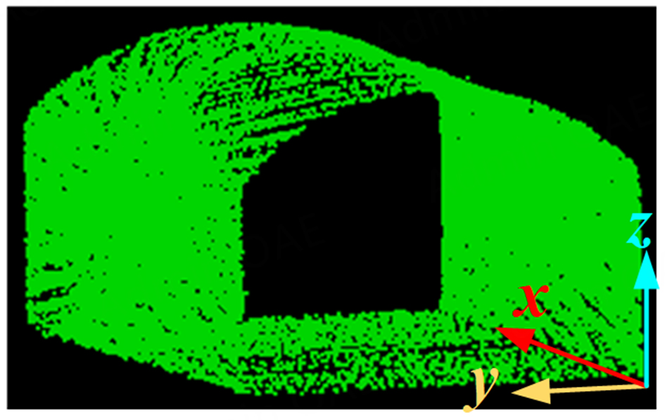
Figure 5. Original point cloud data.
During point cloud simplification, the original point cloud data are simplified via random downsampling, curvature downsampling, voxel grid downsampling, and the method presented in this paper. Figure 6 shows the experimental results.
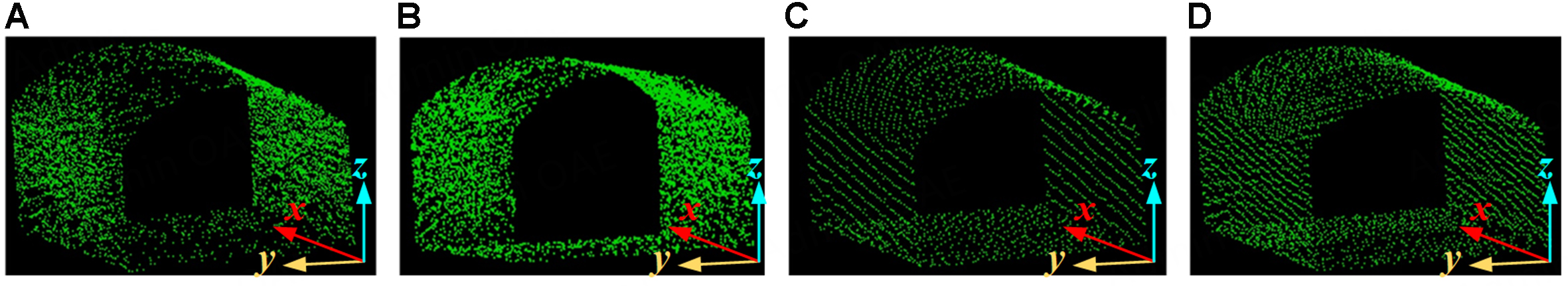
Figure 6. Comparison of different downsampling results. (A) Random downsampling; (B) Curvature-based downsampling; (C) Voxel downsampling; (D) Proposed method in this work.
Figure 6 presents the simplified results of the original point cloud using four algorithms: (a) random downsampling; (b) curvature downsampling; (c) traditional voxel grid downsampling; and (d) optimised voxel grid downsampling. As shown, all four algorithms effectively simplify the original point cloud. To quantitatively analyse their advantages and disadvantages, this paper counts the number of points and calculates the simplification rate and processing time for each algorithm. The results are presented in Table 2.
Comparison of parameter results of different downsampling algorithms
| Method | Number of original points | Number of points after downsampling | Simplification rate/% | Consumption time/ms |
| Random downsampling | 57,070 | 5,707 | 90.00 | 7.98 |
| Curvature downsampling | 5,967 | 89.54 | 3,279.23 | |
| Voxel downsampling | 2,865 | 94.98 | 111.97 | |
| The proposed method in this work | 3,911 | 93.15 | 258.00 |
Consider Figures 5 and 6 and Table 2 together. Although the random downsampling algorithm is quick and reduces the point cloud by 90.00%, it leaves a local area of the point cloud missing. The curvature downsampling algorithm better preserves the detailed features of the original point cloud than the random downsampling algorithm. However, it reduces the point cloud by only 89.54%, and the process takes too long. The traditional voxel grid downsampling algorithm is relatively efficient, with a simplification rate of 94.48%. However, due to defects in its sampling calculation process, some areas of the original point cloud surface have too few points, making it easy to lose small feature information. After processing point cloud data using the optimised voxel grid downsampling algorithm presented in this paper, the reduction rate is slightly lower at 93.15%. This method best preserves the local characteristics of the original point cloud data and has a relatively short processing time, meeting the needs of the downsampling process.
The point cloud downsampling method is usually evaluated based on its accuracy and simplicity. The above content preliminarily analyses the performance of different downsampling algorithms. To evaluate the accuracy of the original point cloud data after processing with different algorithms, the key point retention rate is used as an evaluation index. This rate is defined as the ratio of the number of key points after downsampling to the number of key points before downsampling. Since the intrinsic shape signature (ISS) key point extraction algorithm provides rich geometric feature information and produces high-quality key points, this paper uses it to determine the number of key points before and after downsampling. The corresponding results are shown in Table 3. As shown in Table 3, random downsampling has the lowest key point retention rate among the four downsampling algorithms, consistent with previous findings. The method described in this paper achieves the highest key point retention rate of 68.59%. Therefore, this method better preserves the key points and geometric feature information of a point cloud during simplification.
Key point extraction results of different downsampling algorithms
| Method | Number of original key points | Number of key points after downsampling | Retention rate of key point/% |
| Random downsampling | 554 | 322 | 58.12 |
| Curvature downsampling | 371 | 66.97 | |
| Voxel downsampling | 323 | 58.30 | |
| The proposed method in this work | 380 | 68.59 |
3. DETECTION AND FITTING OF ROADWAY SECTION SHAPE
Roadway deformation detection based on laser scanning primarily uses preprocessed point cloud data to determine overall deformation. However, it is difficult to accurately detect roadway deformation directly from point cloud data. Therefore, deformation is extracted by segmenting the roadway point cloud into multiple sections for local analysis rather than analysing the entire roadway. Deformation detection and analysis are performed by intercepting the entire roadway point cloud. This method eliminates the time-consuming process of placing markers in traditional roadway deformation detection, making the process more efficient and safer. First, the central axis of the entire roadway point cloud is extracted. Then, the point cloud trend is adjusted to be parallel to the central axis, which facilitates section interception based on roadway mileage. Finally, the section point cloud segmentation and contour curve fitting are completed.
3.1. Extraction of roadway central axis
Deformation detection based on roadway point cloud data requires extracting the central axis of the roadway to represent its overall orientation and trend. Using the central axis ensures that the intercepted roadway section is perpendicular to the roadway direction. This ensures that the deformation of the intercepted section reflects the actual deformation at that location along the roadway. Several methods exist for extracting the central axis, including projection-based methods, coarse segmentation iteration, and cubic spline interpolation fitting. Because the projection-based method is simple, convenient, and efficient, this paper presents a method for extracting the roadway central axis based on bidirectional projection. The specific process is as follows:
(1) Extraction of the boundary contour of the projected point cloud: First, the roadway point cloud data is projected onto the xoy and xoz planes. Then, the boundary point set is extracted using the Alpha-Shapes algorithm[22]. As shown in Figure 7, the criterion of the Alpha-Shapes algorithm for identifying boundary points is as follows: a circle with radius α is drawn through any two points P1 and P2 in the point set P. If no other points lie within the circle, P1 and P2 are regarded as boundary points. Given points P1 (x1, y1) and P2 (x2, y2), and the centre of the circle passing through P1 and P2 is denoted as P3 (x3, y3), and the coordinates of P3 can be calculated by[22]
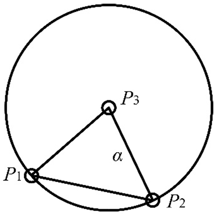
Figure 7. Circle centre solution of the Alpha-Shapes algorithm.
where
Once the coordinates of the centre of the circle are obtained, it is possible to determine whether other points lie within the circle by evaluating the relationship between the distances from other points in the point cloud data to the centre and the radius, α. Figure 8 shows the result of boundary contour extraction from the point cloud data.
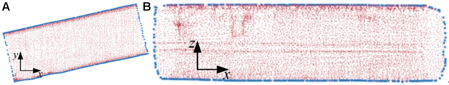
Figure 8. Boundary points extraction of point cloud data. (A) Extracted boundary points in xoy projection; (B) Extracted boundary points in xoz projection.
(2) Central axis extraction
After extracting the projection boundary points of the point cloud, a step length Δx is set along the roadway axis, and sampling is performed at equal intervals to obtain the maximum and minimum values in the y and z directions. Then, the median values in the y and z directions corresponding to xi (i = 1, 2, 3, ..., n) are calculated, and the midpoint set A = {a1, a2, a3, ..., an} in the xoy plane and the midpoint set B = {b1, b2, b3, ..., bn} in xoz are obtained. This can be expressed as
where yi(max), yi(min), zi(max), and zi(min) respectively represent the maximum and minimum values in the y and z directions corresponding to xi; yi(mid) and zi(mid) respectively represent the median values of the corresponding y direction and z direction at xi.
The results of midpoints extraction in the xoy and xoz planes are shown in Figure 9.
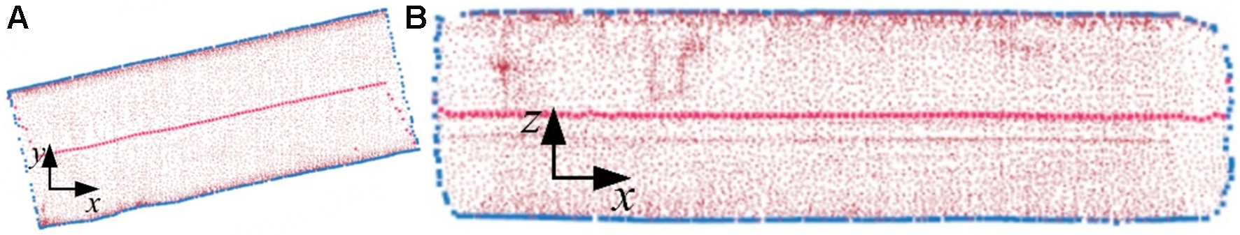
Figure 9. Midpoints extraction of point cloud data. (A) Extracted midpoints in xoy projection; (B) Extraction of midpoints in xoz projection.
(3) Fitting the central axis
Given that the experimental area considered in this paper is a straight-line segment, straight lines are fitted to the midpoint sets in the two planes to obtain the final axis equation. The RANSAC algorithm[23] is used to fit lines to the midpoint sets A and B. The resulting straight-line equations are then used to obtain the central axis equation. The result of the straight-line fitting is shown in Figure 10.
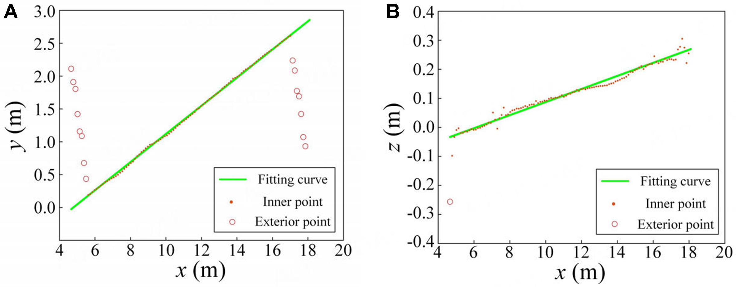
Figure 10. Line fitting results of point sets A and B based on RANSAC. (A) Fitting result of point set A; (B) Fitting result of point set B. RANSAC: Random sample consensus.
Among them, Figure 10A shows the result of the straight-line fitting of point set A, where the straight-line equation is denoted as y = f(x). Figure 10B shows the straight line fitting result of point set B, where the straight-line equation is denoted as z = g(x). Therefore, the central axis equation can be expressed as
3.2. Detection and fitting of roadway profile
To intercept the section point cloud based on roadway mileage information, the overall trend of the point cloud must first be adjusted. As shown in Figure 11, the original point cloud data is not aligned with the coordinate axes. Since the experimental area is a straight line, the point cloud trend is adjusted to be parallel to the x-axis using the central axis of the roadway for subsequent processing.
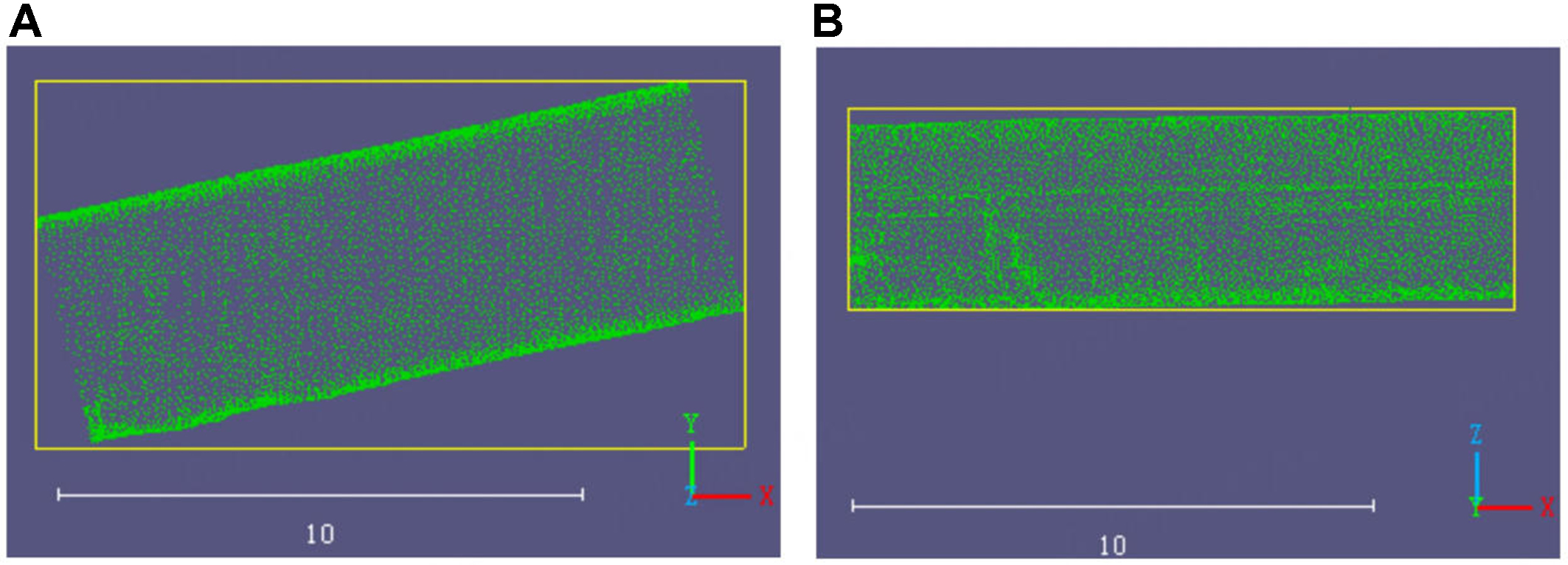
Figure 11. Original point clouds before adjustment. (A) Top view; (B) Front view.
As shown in Figure 11, there is an included angle between the roadway point cloud and the x-axis in both the top and front views. The purpose of adjusting the point cloud is to eliminate this angle and align it with the x-axis. The point cloud attitude angle adjustment method is mainly divided into two parts. The first part is to calculate the included angles between the centreline and the x-axis of the xoy and xoz planes based on the solved central axis equation, and record the angles as α and β, respectively. Second, the point cloud is rotated according to angles α and β to make its overall trend parallel to the x-axis. After adjusting the roadway point cloud to be parallel to the x-axis, the data is imported into the CloudCompare point cloud processing software. The section point cloud is then intercepted, and the contour curve is fitted along the x-axis.
Initially, as illustrated in Figure 12, the point cloud data is segmented into multiple slices based on the parameters set in the point cloud processing software, such as the slice interval and thickness. The envelope curve is used to fit the outline of each intercepted point cloud, which will be used to measure roadway deformation. During cross-section point cloud fitting, each sliced point cloud is projected onto the same cross-section for separate fitting. This prevents interference from other cross-section point clouds when fitting the contour of the current cross-section. Figure 13 shows the contour fitting result of the cross-section point cloud.
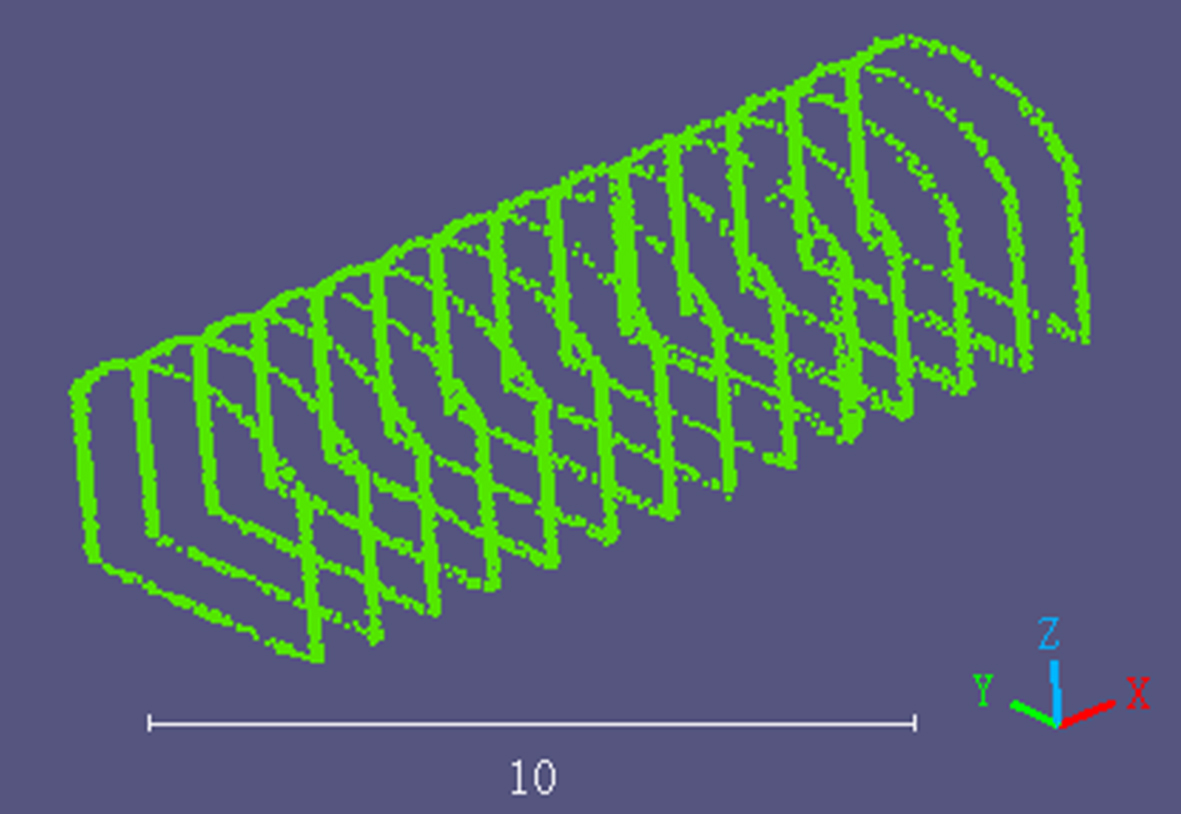
Figure 12. Diagram of segmented point clouds.
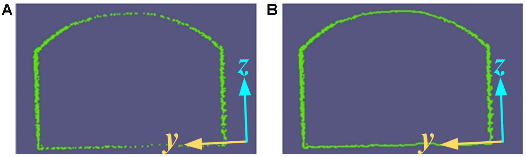
Figure 13. Cross-sectional contour fitting results. (A) Original section point cloud; (B) Fitted section point cloud.
In the domain of roadway deformation detection and analysis, the prevailing approach entails determining surface deformation through the measurement of displacement convergence. This includes measuring roof and floor displacement, as well as the displacement between the two sides. In practice, the “cross” measurement method is frequently employed. The detection targets are arranged on the roof, floor, and sides of the roadway, and the roadway surface deformation is then calculated based on the positions of these targets. Using processed point cloud data of the roadway, this paper references previous methods for monitoring surface displacement to detect roadway deformation. Furthermore, the system integrates comprehensive and local deformation analyses to ascertain the current state of roadway deformation.
Comprehensive Deformation Analysis: 3D point cloud data of the roadway is divided into sections along the axis at set distances and thicknesses. Subsequently, the contour curve of each section’s point cloud is fitted to measure the displacement of the roof and floor, as well as the displacement of the two sides, at different time periods. The comprehensive deformation state of the roadway is obtained by analysing displacement variations between the roof and floor, the roof and sides, and the floor and sides.
Local Deformation Analysis: This involves procuring and examining specific deformation information for a designated section of the roadway. Frequently, multiple measuring points are established along the section to acquire local deformation information at the roof, floor, and two sides through multi-stage monitoring of the positions of the measuring points. In this paper, the section with the greatest deformation is identified through overall deformation analysis by comparing the point cloud data from multiple periods. Subsequently, local deformation information is obtained by establishing multiple measuring points in that section.
4. EXPERIMENT
This paper uses simulated roadway point cloud data obtained by LiDAR scanning of a simulated roadway inspection robot to verify the feasibility of the roadway deformation detection method based on laser scanning. Point cloud section information is extracted using a combination of point cloud processing and roadway shape detection methods. An experimental study of coal mine roadway deformation monitoring is then conducted to detect deformation.
4.1. Data acquisition
To obtain 3D point cloud data of a simulated roadway, an inspection robot equipped with LiDAR scans the environment and detects deformation information. The mean illuminance in the experimental roadway, shown in Figure 14A, is approximately 12.8 Lux. The tunnel remains inactive between scanning phases, ensuring the elimination of additional dust interference. According to the principle of LiDAR ranging, illumination has a negligible impact on LiDAR scanning. As shown in Figure 14A, the data processing method in this study was validated using two scanning periods of data continuously collected at different times along a fixed trajectory in the simulated roadway. The time interval between the two scanning periods was approximately eight months. As shown in Figure 14B and Table 4, the green point cloud data from the initial scan are designated as Phase I data, while the red point cloud data from the scan conducted eight months later are designated as Phase II data.
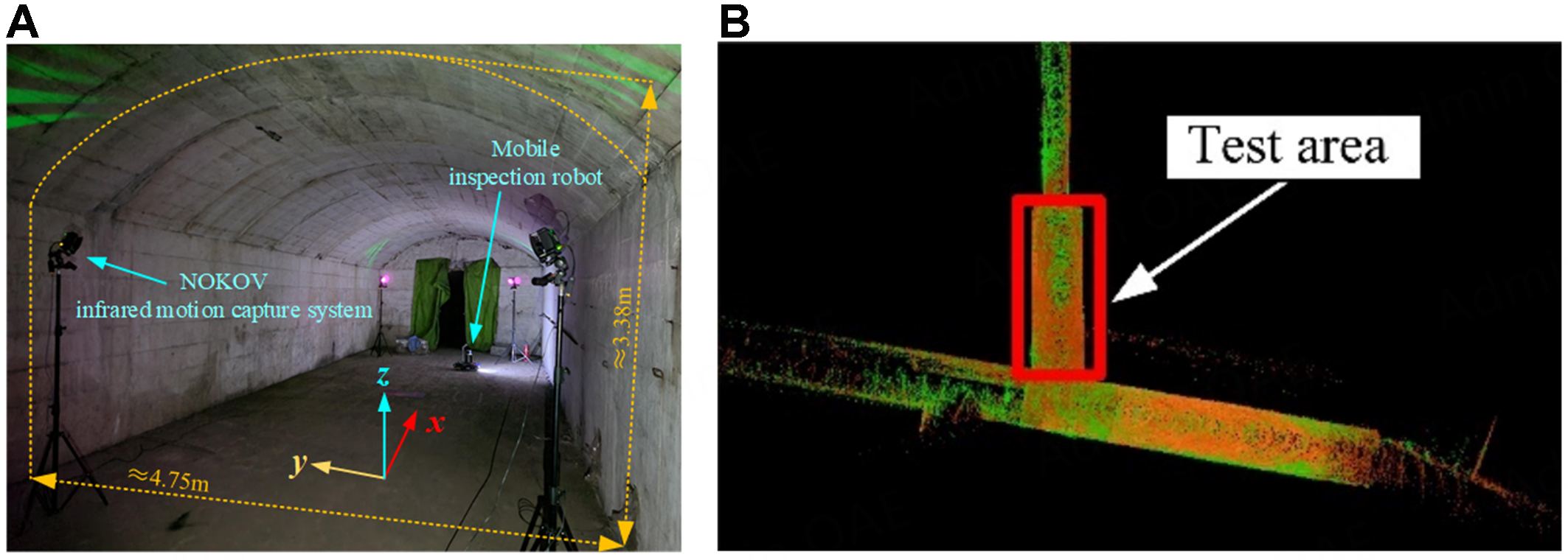
Figure 14. Experimental roadway and its point cloud data. (A) Experimental roadway; (B) Point cloud of the roadway.
Detailed information about point cloud data
| Serial number | Serial name | Mileage/m | Count |
| 1 | First phase I | 14 | 63,391 |
| 2 | Second phase II | 14 | 65,370 |
The accuracy of LiDAR scanning data has a direct impact on the outcomes of deformation detection. The system’s accuracy was verified using a precision infrared motion capture system. The discrepancy between the positions of the markers, as determined by the LiDAR scanning data and the infrared motion capture system, is analyzed to ascertain the extent to which the point cloud measurement accuracy meets the established criteria.
Initially, the environment is scanned using a 3D LiDAR scanner. The centre coordinates of each marker are then obtained by processing the scanned data. The infrared marker is shown in Figure 15. Subsequently, the NOKOV infrared motion capture system (by Beijing NOKOV Science & Technology Co., Ltd., China) measures the centre coordinates of the markers. Its high-performance infrared lens enables the acquisition of 3D object coordinates with submillimeter precision. Consequently, these measured values can be regarded as actual coordinate values. Comparing the coordinate values obtained by the two methods allows the measurement error of the roadway point cloud to be determined. Ten markers were set up on the simulated roadway, and the measured values from the NOKOV infrared motion capture system and LiDAR scanning are shown in Table 5.
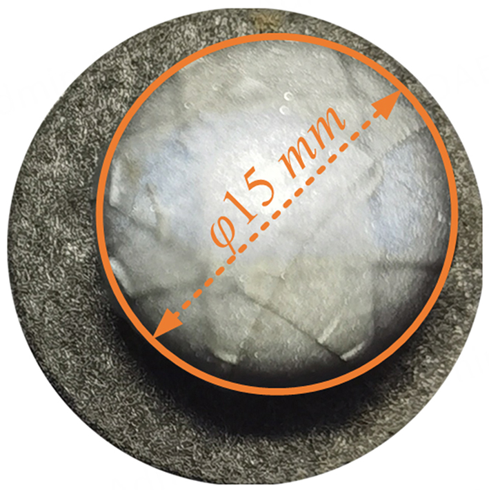
Figure 15. Infrared measuring marker of the NOKOV infrared motion capture system.
Measured coordinates of the markers (Unit: m)
| Number | NOKOV infrared motion capture system | LiDAR scanning | Error (× 10-3) | ||||||
| x | y | z | x | y | z | x | y | z | |
| 1 | 1.9614 | 2.4149 | -0.5505 | 1.9631 | 2.4135 | -0.5519 | 1.7 | -1.4 | -1.4 |
| 2 | 2.1347 | 2.1561 | -0.5537 | 2.1332 | 2.1553 | -0.5522 | -1.5 | -0.8 | 1.5 |
| 3 | 3.3591 | 1.8474 | -0.5823 | 3.3599 | 1.8464 | -0.5835 | 0.8 | -1.0 | -1.2 |
| 4 | 5.8422 | 1.8181 | -0.7585 | 5.8436 | 1.8171 | -0.7571 | 1.4 | -1.0 | 1.4 |
| 5 | 6.5032 | 1.4308 | 0.0801 | 6.5022 | 1.4319 | 0.0791 | -1.0 | 1.1 | -1 |
| 6 | 4.5225 | 0.6365 | -0.0606 | 4.523 | 0.6349 | -0.0599 | 0.5 | -1.6 | 0.7 |
| 7 | 4.2929 | 0.2278 | -0.7211 | 4.2948 | 0.2258 | -0.7223 | 1.9 | -2.0 | -1.2 |
| 8 | 4.2679 | 0.6486 | 0.6174 | 4.2664 | 0.6501 | 0.6190 | -1.5 | 1.5 | 1.6 |
| 9 | 3.2423 | 0.5627 | -0.5142 | 3.2409 | 0.5620 | -0.5159 | -1.4 | -0.7 | -1.7 |
| 10 | 3.8128 | 2.8844 | 1.2562 | 3.8141 | 2.8852 | 1.2556 | 1.3 | 1.7 | -0.6 |
The difference, shown in the last column of Table 5, between the marker coordinates obtained from LiDAR scanning and those measured by the NOKOV infrared motion capture system reveals the deviation of the laser scanner along the three axes. According to Table 5, the coordinate errors at the same positions using the two devices are less than 2 mm. The absolute average errors of the LiDAR scanning measurements on the x, y, and z axes are 1.30, 1.19, and 1.23 mm, respectively. Given the significant deformation of the roadway, the accuracy of the 3D laser scanning measurements presented in this paper meets the required standards.
4.2. Preprocessing of roadway point cloud
Original point cloud data often contains noise points on the surface contours of non-simulated roadways. This hinders the subsequent extraction and analysis of roadway contour characteristics. Accordingly, this paper presents a method for denoising and downsampling point clouds to preprocess the original data in two experimental areas. First, a combined statistical and median filtering method is used to remove large- and small-scale noise from the original point cloud data. Figure 16 shows that the combined filtering method effectively eliminates unnecessary noise points while preserving the detailed features of the original point cloud data, providing a basis for subsequent processing.
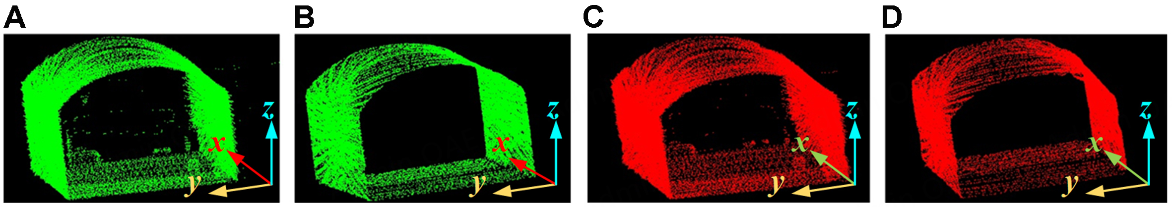
Figure 16. Denoising results of the point clouds of Phase I and Phase II. (A) Original Phase I; (B) Denoised Phase I; (C) Original Phase II; (D) Denoised Phase II.
Although point cloud combination filtering removes some noisy points, the original point cloud data remains dense with many points. In this paper, analysing and processing simulated roadway point cloud data does not require such high density. Additionally, high-density point clouds increase the data processing burden in later stages and reduce computational efficiency. Based on point cloud denoising, the point cloud data is further simplified using density constraints and downsampling of neighbouring points around the centre of gravity of the voxel grid. Figure 17 shows the results of point cloud downsampling. After downsampling, the number of point clouds of Phase I and Phase II is reduced to 4,431 and 4,313, respectively.
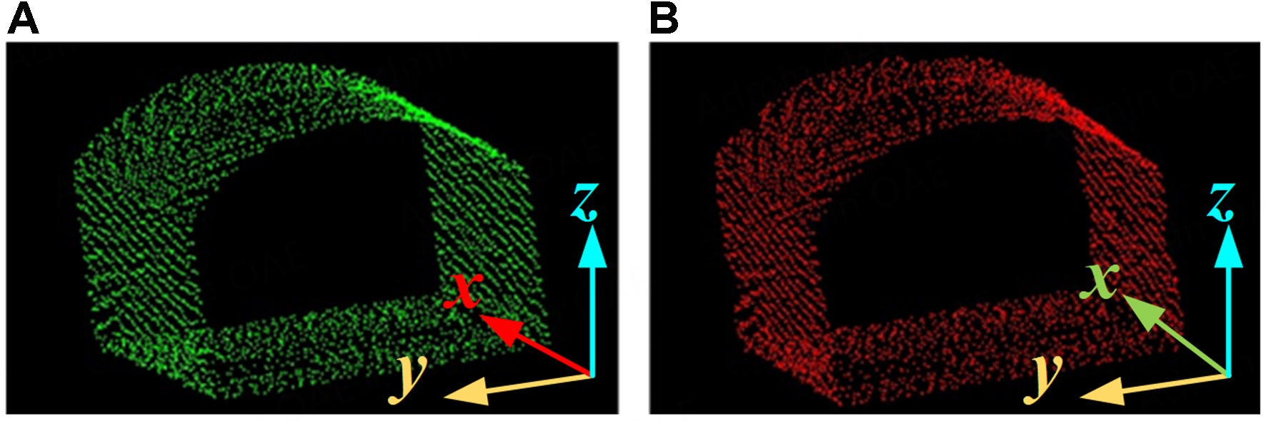
Figure 17. Downsampling results of the point clouds of Phase I and Phase II. (A) Downsampled Phase I; (B) Downsampled Phase II.
4.3. Detection results of roadway contour
Firstly, the central axis of the roadway is extracted using the bidirectional projection method based on the point cloud data preprocessed in the previous section. Subsequently, the point cloud orientation is adjusted using CloudCompare. The point cloud of the roadway section is then intercepted and fitted. The two-stage point cloud data of the simulated roadway are first projected onto the xoy and xoz planes, respectively. In the next stage, the boundary contour point set of the projected point cloud is extracted using the Alpha-Shapes algorithm. The axis point set is then extracted using the median method. The central axis point sets obtained from the xoy and xoz planes are fitted with straight lines using the RANSAC algorithm to obtain the central axis equations of the point clouds of Phase I and Phase II:
According to the central axis equations, the angles α between the projected point cloud trend on the xoy plane and the x axis are 12.189° and 12.024°, respectively, and the angles β between the projected point cloud attitude trend on the xoz plane and the x axis are 1.203° and 1.146°, respectively. The two-stage point cloud data of the simulated roadway are imported into the point cloud processing software, and the point cloud orientation is adjusted to be parallel to the x-axis based on the angles α and β.
Because the point clouds are discrete and not evenly distributed in space, it is impossible to ensure that there are enough points to maintain the integrity of each section. Therefore, it is necessary to interpolate the point cloud data with a certain thickness to ensure section integrity during extraction. Considering the scale of the experimental area, sections with slice thicknesses d of 5, 10, 15 and 20 cm are selected for comparison, as shown in Figure 18. As shown, when the slice thickness is d = 5 cm or d = 10 cm, the contour retention of the section point cloud is worse than when d = 15 cm or d = 20 cm. When d = 20 cm, the intercepted section contains more points, but compared with d = 15 cm, there is little difference in the effectiveness of preserving the profile of the section point cloud. Therefore, a slice thickness of d = 15 cm is selected to extract the roadway section. Thirteen cross-sectional point clouds are extracted from the two-phase point clouds in the experimental area, each spaced one meter apart. The thickness of each cross-sectional point cloud is set to
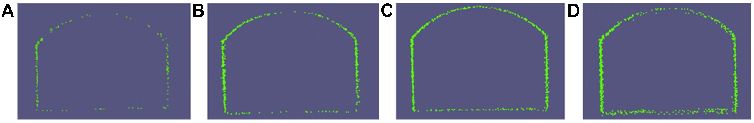
Figure 18. Influence of different slice thicknesses on the contour retention of section point clouds. (A) d = 5 cm; (B) d = 10 cm; (C) d =

Figure 19. Section extraction and contour fitting results.
4.4. Deformation analysis of roadway
A comparative analysis was conducted based on the extracted information from two sections of a simulated roadway. The “cross” measurement method was used to determine the change in distance between the roof and floor and between the roof and the two sides of each section, with the objective of detecting and analysing deformation in the entire regional section. As shown in Table 6, the distances between the roof and floor, as well as between the roof and the two sides of the simulated roadway, are presented for two distinct periods. To provide a clearer illustration of the trend in distance changes, a diagram of the displacement convergence trend was drawn based on the point cloud data collected in Phase I and the section parameters in Table 6. The overall section deformation results are displayed in Figure 20.
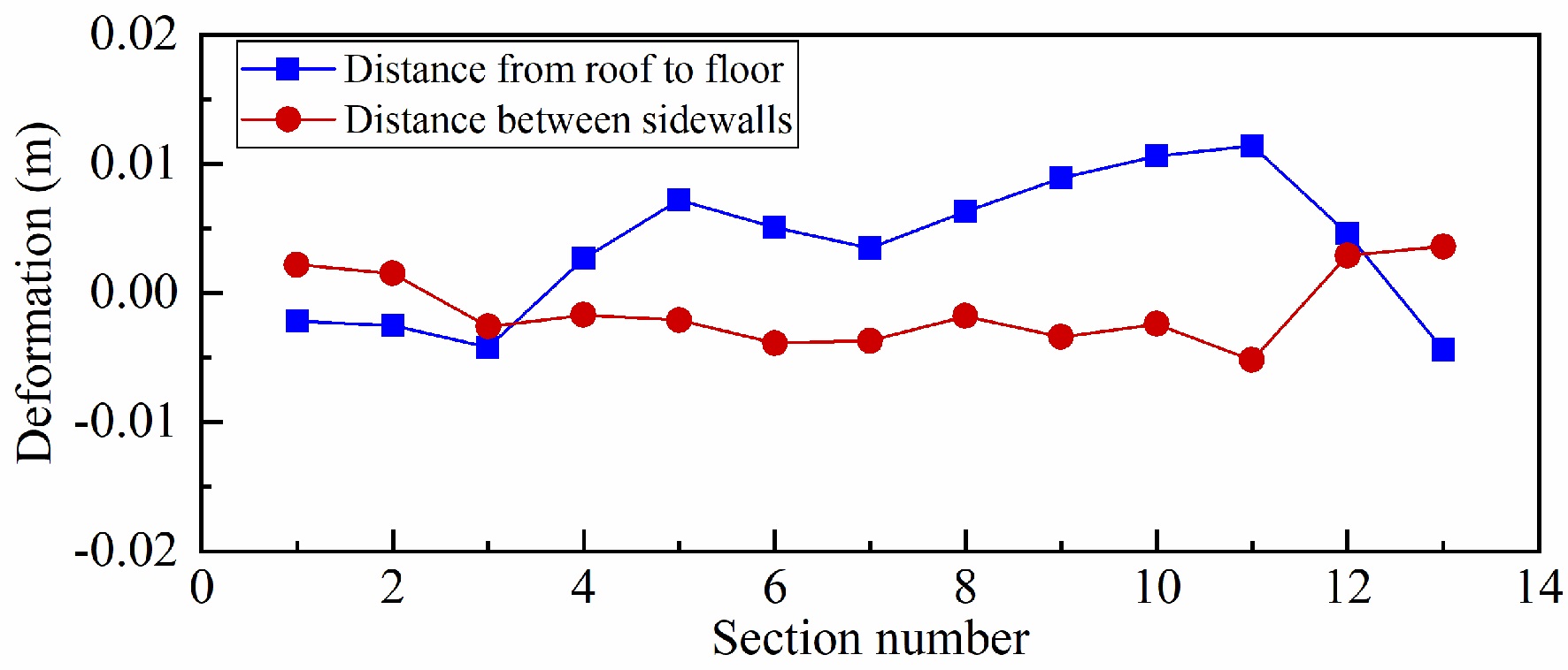
Figure 20. Overall section deformation results from Phase I to Phase II.
Section deformation parameters of the two phases of the roadway
| Section number | Distance from roof to floor in Phase I/m | Distance from roof to floor in Phase II/m | Distance between sidewalls in Phase I/m | Distance between sidewalls in Phase II/m |
| 1 | 3.3871 | 3.3893 | 4.7833 | 4.7811 |
| 2 | 3.3769 | 3.3794 | 4.7756 | 4.7741 |
| 3 | 3.3799 | 3.3841 | 4.7572 | 4.7598 |
| 4 | 3.3813 | 3.3786 | 4.7473 | 4.749 |
| 5 | 3.3617 | 3.3545 | 4.7378 | 4.7399 |
| 6 | 3.3889 | 3.3838 | 4.7252 | 4.7291 |
| 7 | 3.4309 | 3.4274 | 4.7295 | 4.7332 |
| 8 | 3.3635 | 3.3572 | 4.7431 | 4.7449 |
| 9 | 3.4188 | 3.4099 | 4.7643 | 4.7677 |
| 10 | 3.3408 | 3.3302 | 4.7522 | 4.7546 |
| 11 | 3.3949 | 3.3835 | 4.7539 | 4.7591 |
| 12 | 3.3647 | 3.3601 | 4.718 | 4.7151 |
| 13 | 3.3821 | 3.3865 | 4.7001 | 4.6965 |
As shown in Table 6 and Figure 20, the distance between the roof and floor, as well as between the two sides, varies across the 13 sections. Notably, the distance between the roof and floor exhibited greater variability than the distance between the two sides during the two data periods. The mean deformation of the roof and floor was 5.7 mm, while the mean deformation of the two sides was 1.3 mm. Furthermore, section 11 shows substantial deformation of the roof, floor, and two sides, with measurements of 11.4 and 5.2 mm, respectively. Consequently, local deformation requires continuous monitoring and analysis. To measure the deformation of section 11’s roof, floor, and sides conveniently, the contour curve of the first section is used as a reference. In the subsequent stage, the second section’s contour curve is compared with the first section’s curve. This process enables the extraction of deformation for each part. Following a detailed comparison of the profile curves of the two sections, a total of 12 groups of data were sampled at intervals along the top, bottom, left, and right axes. The absolute deformation parameters of each part are shown in Table 7, and the deformation curve is shown in Figure 21. As shown in Table 7 and Figure 21, the mean deformation of the roof, floor, left side, and right side is 6.8, 4.0, 2.4, and 3.4 mm, respectively. Because the roof is exposed to significantly higher pressure compared with other areas, it undergoes greater deformation.
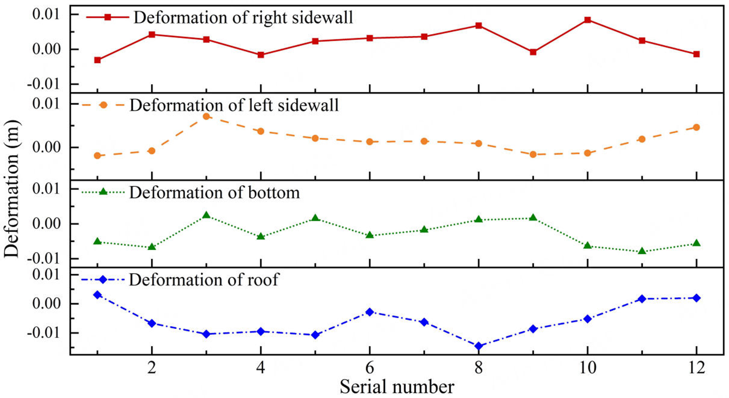
Figure 21. Local deformations from Phase I to Phase II.
Local deformation parameters of two-stage section
| Serial number | Deformation of roof/mm | Deformation of bottom/mm | Deformation of left sidewall/mm | Deformation of right sidewall/mm |
| 1 | 3.1 | 5.2 | 1.9 | 3.1 |
| 2 | 6.7 | 6.8 | 0.8 | 4.2 |
| 3 | 10.4 | 2.3 | 7.1 | 2.8 |
| 4 | 9.5 | 3.8 | 3.7 | 1.6 |
| 5 | 10.7 | 1.5 | 2.1 | 2.3 |
| 6 | 2.8 | 3.4 | 1.3 | 3.2 |
| 7 | 6.3 | 1.8 | 1.4 | 3.6 |
| 8 | 14.5 | 1.1 | 0.9 | 6.8 |
| 9 | 8.6 | 1.6 | 1.6 | 0.8 |
| 10 | 5.2 | 6.4 | 1.3 | 8.4 |
| 11 | 1.7 | 8.0 | 1.9 | 2.5 |
| 12 | 2.0 | 5.7 | 4.6 | 1.4 |
5. CONCLUSIONS
To address elastic and plastic deformation in coal mine tunnel profiles caused by geological conditions and time-varying loads, a laser scanning-based tunnel deformation detection method is proposed. This method achieves effective extraction of LiDAR point clouds by integrating point cloud denoising techniques - namely, statistical and median filtering - with voxel grid subsampling based on density constraints and centroid proximity. The dual-projection method is employed to extract the tunnel centreline. CloudCompare is used for the regional segmentation of point cloud data, facilitating the extraction of tunnel cross-sections and the subsequent fitting of contour curves. This enables monitoring of deformations in the tunnel roof, floor, and sidewalls. The experimental verification process, conducted using an inspection robot platform, showed that the proposed LiDAR-based deformation detection method achieves sub-centimetre accuracy. The LiDAR scanning measurement error of 2 mm meets the requirements for monitoring deformation in coal mine tunnels. Following two phases of roadway environmental scanning conducted at eight-month intervals, the average deformation of the roof and floor was 5.7 mm. In contrast, the average deformation of the sidewalls was 1.3 mm.
DECLARATIONS
Authors’ contributions
Made substantial contributions to the conception and design of the study and performed data analysis and interpretation: Cui, Y.; Yang, G.; Dai, Y.
Performed data acquisition and provided administrative, technical, and material support: Yuan, K.; Liu, X.
Availability of data and materials
The data supporting the findings of this study are available from the corresponding author upon reasonable request.
Financial support and sponsorship
This work was supported in part by the Fundamental Research Funds for the Central Universities (CHD) (Grant 300102255508), in part by the Basic Research Program of Jiangsu (Grant BK20230688), and in part by the Research Fund for Doctoral Degree Teachers of Jiangsu Normal University, China (Grant 22XFRS011).
Conflicts of interest
All authors declared that there are no conflicts of interest.
Ethical approval and consent to participate
Not applicable.
Consent for publication
Not applicable.
Copyright
© The Author(s) 2026.
REFERENCES
1. Jacobson, A.; Zeng, F.; Smith, D.; Boswell, N.; Peynot, T.; Milford, M. What localizes beneath: a metric multisensor localization and mapping system for autonomous underground mining vehicles. J. Field. Robot. 2021, 38, 5-27.
2. Mukupa, W.; Roberts, G. W.; Hancock, C. M.; Al-Manasir, K. A review of the use of terrestrial laser scanning application for change detection and deformation monitoring of structures. Surv. Rev. 2017, 49, 99-116.
3. Yang, H.; Xu, X. Intelligent crack extraction based on terrestrial laser scanning measurement. Meas. Control. 2020, 53, 416-26.
4. Yasuda, N.; Cui, Y. Deformation estimation of a circular tunnel from a point cloud using elliptic Fourier analysis. Tunn. Undergr. Space. Technol. 2022, 125, 104523.
5. Cui, Y.; Liu, S.; Li, H.; Gu, C.; Jiang, H.; Meng, D. Accurate integrated position measurement system for mobile applications in GPS-denied coal mine. ISA. Trans. 2023, 139, 621-34.
6. Dong, J.; Qin, Y.; Xie, Z. Research on risk identification and early warning of bolt failure in coal mine roadway. IEEE. Sens. J. 2025, 25, 19192-202.
7. Wang, Q.; Su, G.; Ma, Q.; Yin, H.; Liu, Z.; Lv, C. Automatic monitoring system for 3-D deformation of crustal fault based on laser and machine vision. Instrumentation 2024, 11, 44-52.
8. Li, J.; Qu, Z.; Wang, S. Y.; Xia, S. F. YOLOX-RDD: a method of anchor-free road damage detection for front-view images. IEEE. Trans. Intell. Transport. Syst. 2024, 25, 14725-39.
9. Yan, K.; Wang, J.; Wang, J.; Tian, D.; Peng, S.; Xu, Y. An efficient improved Yolov5-based method for detecting iron waste in ores. Instrumentation 2025, 12, 36-46.
10. Zhao, D.; Yao, H.; Gu, X. Highway deformation monitoring by multiple InSAR technology. Sensors 2024, 24, 2988.
11. Pu, J.; Yu, Q.; Zhao, Y.; et al. Deformation analysis of a roadway tunnel in soft swelling rock mass based on 3D mobile laser scanning. Rock. Mech. Rock. Eng. 2024, 57, 5177-92.
12. Ji, C.; Sun, H.; Zhong, R.; Li, J.; Han, Y. Precise positioning method of moving laser point cloud in shield tunnel based on bolt hole extraction. Remote. Sens. 2022, 14, 4791.
13. Ji, C.; Sun, H.; Zhong, R.; Sun, M.; Li, J.; Lu, Y. Deformation detection of mining tunnel based on automatic target recognition. Remote. Sens. 2023, 15, 307.
14. Singh, S. K.; Raval, S.; Banerjee, B. A robust approach to identify roof bolts in 3D point cloud data captured from a mobile laser scanner. Int. J. Min. Sci. Technol. 2021, 31, 303-12.
15. Maes, K.; Salens, W.; Feremans, G.; Segher, K.; François, S. Anomaly detection in long-term tunnel deformation monitoring. Eng. Struct. 2022, 250, 113383.
16. Luo, W.; Li, L. Automatic geometry measurement for curved ramps using inertial measurement unit and 3D LiDAR system. Autom. Constr. 2018, 94, 214-32.
17. Morago, B.; Bui, G.; Le, T.; Maerz, N. H.; Duan, Y. Photograph LIDAR registration methodology for rock discontinuity measurement. IEEE. Geosci. Remote. Sensing. Lett. 2018, 15, 947-51.
18. Hu, D.; Li, Y.; Yang, X.; et al. Experiment and application of NATM tunnel deformation monitoring based on 3D laser scanning. Struct. Control. Health. Monit. 2023, 2023, 1-13.
19. Cui, H.; Ren, X.; Mao, Q.; Hu, Q.; Wang, W. Shield subway tunnel deformation detection based on mobile laser scanning. Autom. Constr. 2019, 106, 102889.
20. Lu, J.; Wang, W.; Fan, Z.; Bi, S.; Guo, C. Point cloud registration based on CPD algorithm. In 2018 37th Chinese Control Conference (CCC), Wuhan, China. July 25-27, 2018. IEEE; 2018. pp. 8235-40.
21. Tao, S.; Bai, R. Point cloud registration method based on key point optimization after downsampling. Appl. Res. Comput. 2021, 38, 904-7. (in Chinese).
22. dos Santos, R. C.; Pessoa, G. G.; Carrilho, A. C.; Galo, M. Automatic building boundary extraction from airborne LiDAR data robust to density variation. IEEE. Geosci. Remote. Sensing. Lett. 2022, 19, 1-5.
Cite This Article
How to Cite
Download Citation
Export Citation File:
Type of Import
Tips on Downloading Citation
Citation Manager File Format
Type of Import
Direct Import: When the Direct Import option is selected (the default state), a dialogue box will give you the option to Save or Open the downloaded citation data. Choosing Open will either launch your citation manager or give you a choice of applications with which to use the metadata. The Save option saves the file locally for later use.
Indirect Import: When the Indirect Import option is selected, the metadata is displayed and may be copied and pasted as needed.
About This Article
Copyright

Data & Comments
Data
0


Comments
Comments must be written in English. Spam, offensive content, impersonation, and private information will not be permitted. If any comment is reported and identified as inappropriate content by OAE staff, the comment will be removed without notice. If you have any queries or need any help, please contact us at [email protected].