Convolutional neural network aided movable antenna array design for channel estimation

1. INTRODUCTION

Massive multiple-input multiple-output (MIMO) is considered as a crucial technology by employing an enormous number of antennas in the fifth-generation (5G) communication and beyond, and the independent data streams are transmitted to implement the spatial multiplexing gain^[1]. Nevertheless, the associated high hardware cost and power consumption render it practically infeasible in more complex wireless communication scenarios. With the fast development of wireless communications, the tendency of various signal processing techniques is going to provide a greater degree of freedom (DoF) for the desired gain in the corresponding aspects. The core principle is to employ the spatial properties to enhance the overall performance of communication and sensing^[2]. Although the advantages of the sparse arrays compared to the traditional fixed position arrays (FPAs) have been evaluated in deterministic and stochastic channel models, the non-uniform nature of terahertz channels and reconfigurable intelligent surface (RIS)^[3] is investigated for movable antenna (MA)-based designs to guarantee satisfactory conditions of the transmitted signal and propagation environment.

To guarantee reliable and high-quality services for the users in the sixth-generation (6G) system, MAs have attracted more attention in the upcoming 6G networks since they can reconfigure the spatial channel environment, such as constructive or destructive path interference, path orthogonalization, and signal transmission condition through adjusting the antenna positions by flexible cables to the radio frequency (RF) chain^[4]. Similar to the MAs, the fluid antennas aim to improve the inherent capabilities of channels via the optimization of antenna position based on the signal processing technologies^[5,6]. Both the fluid and MAs depend on a similar operating principle and their widespread employment is implemented in modern communication applications.

Compared to the FPAs, the performance generated by the MAs has been analyzed comprehensively and it is better especially in multi-user and multi-antenna scenarios^[7–11]. The beamforming tasks are realized in downlink cases^[12,13], uplink cases^[14,15] and MIMO^[16,17], under different types of constraints. Specifically, the trade-off between the maximization of antenna array gains towards the desired directions and the minimization of sidelobe interference in undesired directions is achieved in multiple beamforming design based on the movable array^[7]. Moreover, for the multiple-input single-output (MISO) system where the MA array is configured with the base station (BS), the joint optimization of the antenna location and weighting coefficients is achieved and therefore the total consumed power is minimized^[18]. For the single-input multiple-output (SIMO) system, the minimization of total transmitted power^[12] and the maximization of minimum achievable rate^[15] are both implemented via jointly optimizing the antenna position, the transmission power of the users and the received beamforming vector. However, the above antenna array designs require iterative computation with high complexity which results in significant challenges for implementation in practical applications^[19].

Recently, a series of deep learning (DL) algorithms have been proposed to develop antenna array designs based on MAs^[20–22]. A joint optimization of the antenna locations and channel state functions is achieved by a deep neural network which is employed to imitate a decomposed model for received pilot so that both the estimation efficiency and computation efficiency are improved as the outcome^[21]. Due to the high nonconvexity of the formulation which is to optimize the antenna position and antenna weighting coefficients simultaneously, a DL model with unsupervised training strategy is utilized to implement beamforming tasks in a multicast scenario^[4]. Moreover, a multi-agent deep deterministic policy gradient (MADDPG) is developed to realize joint optimization of transmit beamforming and antenna locations in a multi-user communication system^[23].

In this work, a novel MA array design, including the linear and planar arrays, based on the convolutional neural network (CNN)^[24,25] is proposed to reduce the computational complexity because only simple matrix multiplications and function employment are required in mathematical computation rather than the complicated matrix inversion computation. Comparative experiments with three other methods, including linear regression (LR) model^[26], least squares (LS) method^[27] and orthogonal matched pursuit (OMP)^[16] channel estimation method are conducted to analyze and evaluate overall channel properties. Although the OMP method combined with the regularized zero-forcing (ZF) framework is investigated to implement the MA array design with satisfactory performance, it costs much longer time in dealing with the antenna array design whose number of antennas is increased even a few^[16]. Instead, CNNs give a trade-off between the mean square error (MSE) and consumed time for the array design based on MAs^[28], and a novel scheme based on it is developed to achieve channel estimation in this work.

Without loss of generality, this study introduces lightweight CNNs into channel estimation for MA arrays innovative, demonstrating the three major advantages of artificial intelligence (AI) in spatial information systems^[29–32]: First, CNNs can replace the traditional high-complexity iterative solvers with a single forward pass, enabling nonlinear mapping learning; Moreover, the network can be generalized to different orbital geometries such as Low Earth Orbit (LEO)/Medium Earth Orbit (MEO)/Geostationary Earth Orbit (GEO) or terrestrial High-Altitude Platform Stations (HAPS) without the need to redesign or optimize algorithms. Furthermore, the model is compact in size and fast in inference speed, meeting the dual requirements of real-time performance and lightweight design for spaceborne/airborne platforms.

This work focuses on the joint optimization of antenna position and the corresponding weighting coefficients, driven by the following three main contributions:

• First, CNNs accept the real-valued combination of antenna position vectors (APVs) and antenna weighting vectors (AWVs) and output the complex-valued channel matrices for the MA arrays.

• Moreover, joint handling of linear and planar geometries with a single model is achieved and the superiority of the MA in different dimensions is analyzed.

• Compared to the OMP method, CNNs have much higher operation speed for the MA arrays and they give relatively lower MSE for channel estimation.

The remaining part of this work is organized as follows. In Section 2, an introduction of the system model including channel model and CNN is provided. The proposed methods for the joint optimization of antenna positions and weighting coefficients are introduced in Section 3. Additionally, numerical results are presented in Section 4 and conclusions are drawn in Section 5.

2. SYSTEM MODEL

2.1. Channel model

A downlink communication scenario is considered in this section, where the BS equipped with $$ M $$ MAs provides communication services towards $$ Q $$ users and each user is equipped with a fixed antenna. The MAs belonging to the BS are distributed along the $$ x $$ plane and $$ x $$-$$ z $$ plane for the linear and planar arrays, respectively. Suppose that the outline of the moving region of MAs for the planar array is a square and each side length for this square is represented by $$ G $$, which is also the moving size of the linear array case.

Taking the BS as the center, the users are randomly scattered around it, as shown in Figure 1. For simplicity, it is assumed in this process that for both linear and planar arrays the condition of far-field communication between the users and the BS is satisfied; i.e., the users are distributed within the coverage area of the BS, whose transmit power is sufficient. This work pays more attention to the users' direction with the BS, and the distance is implicitly modeled through path loss. Note that the size of MA moving regions is much smaller than that of covering area of the BS.

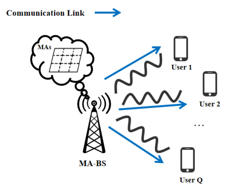
Figure 1. Illustration of the downlink scenario for the BS configured with MAs. BS: Base station; MAs: movable antennas.

In this system, the BS sends transmission signals to different users, and therefore the received signal $$ y_{q} $$ of the $$ q $$-th user, where $$ q \in \{1, \dots, Q\} $$, can be expressed as^[16]

(1) $$ \begin{aligned} &y_q={\boldsymbol{g}}_q^{H}{\boldsymbol{w}}s_q+n_q, \end{aligned} $$

where $$ \boldsymbol{g}_q \in C^{M \times 1} $$ denotes the channel vector of the $$ q $$-th user, $$ H $$ represents the Hermitian transpose, $$ \boldsymbol{w} \in C^{M \times 1} $$ indicates the AWV, $$ s_q $$ signifies the data sent from the BS to the $$ q $$-th user with $$ \boldsymbol{s}=[s_1, \dots, s_Q]^{T}\in C^{Q \times 1} $$ and $$ n_q $$ represents the additive Gaussian white noise (AGWN) with zero-valued mean and variance $$ \sigma^2 $$ at the user side.

Since the MA system relies on the spatial channel model, it is assumed that there are $$ P $$ individual paths between the BS and the user. The channel vector is given by^[16]

(2) $$ \begin{aligned} {\boldsymbol{g}}_q=\frac{1}{\sqrt{P}} \sum\limits_{p=0}^{P-1}\alpha_{q, p} {\boldsymbol{d}} (\theta_{q, p}, \phi_{q, p}), \end{aligned} $$

where $$ \alpha_{q, p} $$ denotes the complex path gain for the $$ q $$-th user in the $$ p $$-th path, and $$ \upsilon $$ and $$ \nu $$ are both the intermediate angular variables, which are used to construct the steering vector (SV) of the MA array, $$ \phi_{q, p}=\sin(\upsilon_{q, p})\sin(\nu_{q, p}) $$ and $$ \theta_{q, p}=\cos(\nu_{q, p}) $$ represent the azimuth and elevation angles of arrival (AoA) of the $$ p $$-th path in the $$ q $$-th user's channel, and $$ \boldsymbol{d} \in C^{M \times 1} $$ denotes the SV of the antenna array, given by^[16]

(3) $$ \begin{aligned} &{\boldsymbol{d}}(\theta_{q, p}, \phi_{q, p})=[e^{-j \frac{2\pi}{\lambda} (\phi_{q, p}x_1+\theta_{q, p}z_1)}, ..., e^{-j \frac{2\pi}{\lambda} (\phi_{q, p}x_{m_x}+\theta_{q, p}z_{m_z})}, ..., e^{-j \frac{2\pi}{\lambda} (\phi_{q, p}x_{M_x}+\theta_{q, p}z_{M_z})}]^{T}, \end{aligned} $$

where $$ (x_{m_x}, z_{m_z}) $$ represents the position of the $$ (m_x, m_z) $$-th MA in the BS with $$ m_x \in \{1, \dots, M_x\} $$ and $$ m_z \in \{1, \dots, M_z\} $$, $$ \lambda $$ and $$ T $$ represent the signal wavelength of the transmitted signal and the transpose operation, respectively.

Since the APV and AWV are highly coupled, the optimal AWV depends instantaneously on the APV through the SV $$ \boldsymbol{d}(\theta_{q, p}, \phi_{q, p}) $$, and vice versa. To capture this non-convex mapping from (APV, AWV) to the channel matrix $$ H $$ without deriving explicit gradients, we adopt a CNN method, and the mapping enables the CNN to handle variations in antenna positions continuously rather than on a discrete grid. Because the joint optimization problem is high-dimensional and strongly coupled, conventional iterative methods are prone to local minima, whereas the proposed CNN-based approach offers superior performance and robustness in MA array design.

2.2. CNN model

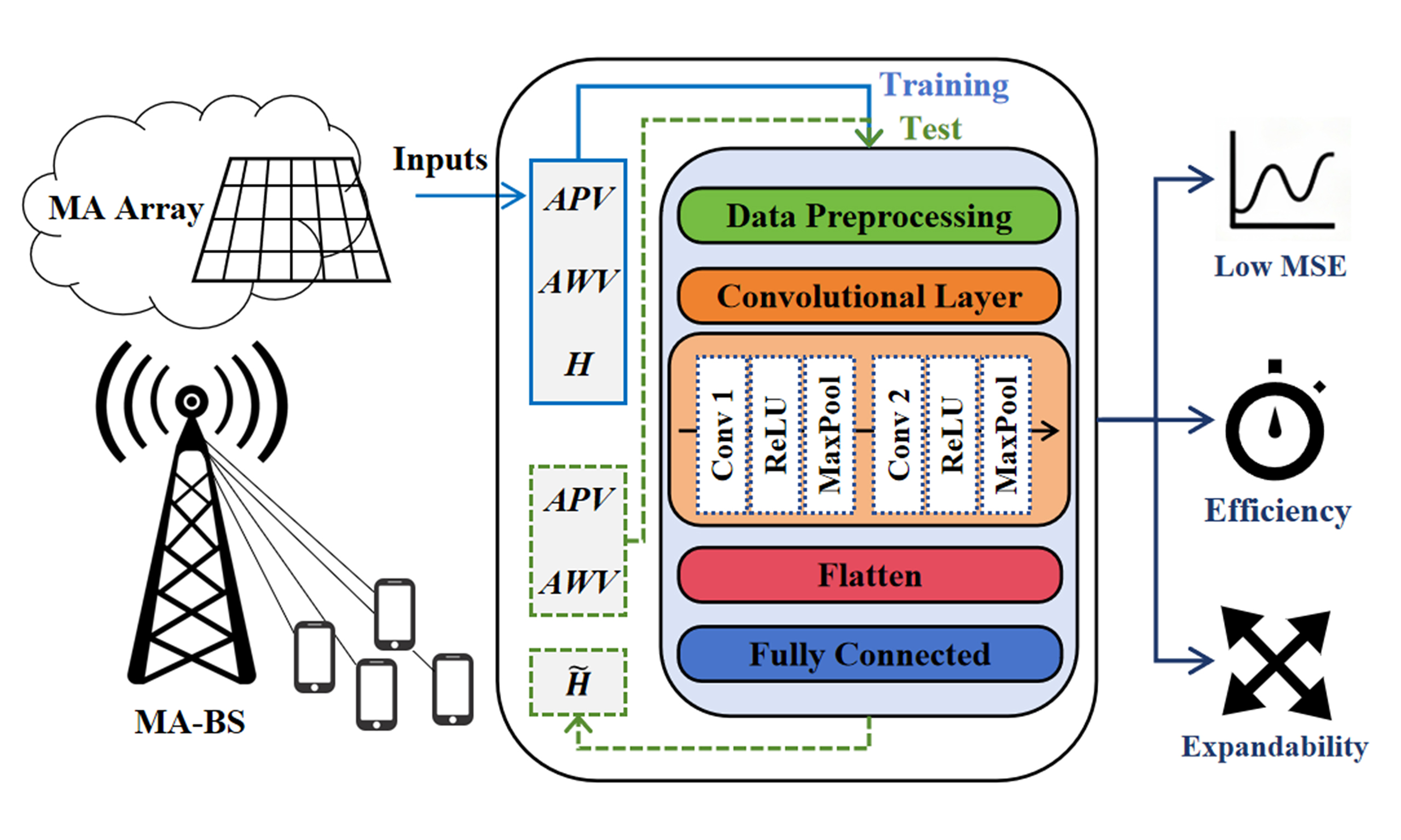
A CNN model based on a one-dimensional (1D) convolutional layer is employed to learn the nonlinear relationship among various variables in the MA wireless communication model; the lightweight structure employed in this work is intentionally shallow to ensure low-latency and low-complexity execution on edge devices. The inputs of the network include the channel matrix $$ H $$, APVs and AWVs, and the output is the channel matrix under the current conditions.

As shown in Figure 2, the processed data is fed through the input layer, which enters the convolutional layer of the model, where Re{} and Im{} denote the real and imaginary parts, respectively. The model consists of two 1D convolutional layers, including Conv $$ 1 $$ and Conv $$ 2 $$. In detail, the Conv $$ 1 $$ employs 32 filters, whose size of the convolutional kernel is $$ 3 $$ and the stride is $$ 1 $$, while the activation function is rectified linear unit (ReLU), which can effectively alleviate the problem of gradient disappearance, introduce beneficial sparsity which improves robustness to anomalous antenna configurations and accelerate the training process of the model. The activation function is given by^[21]

(4) $$ \begin{aligned} f(x)=max(0, x), \end{aligned} $$

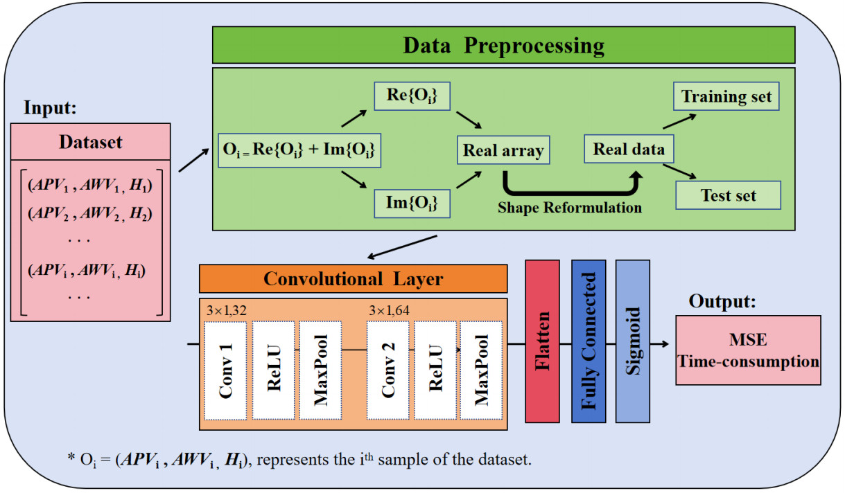
Figure 2. Illustration of the proposed CNN model. CNN: Convolutional neural network.

where max() denotes the function aiming to find the maximum value among several items. Moreover, the Conv 2 uses 64 filters while retaining the size of kernels and the activation function, so as to further extract data features, resulting in receptive field spans and allowing higher-order mutual coupling effects to be modeled. After feature extraction, the output of the convolutional layer is converted into a vector by using the flatten layer, which is convenient for the subsequent connection of the fully connected Layers. There are two fully connected layers, where the first fully connected layer consists of 128 neurons, as the Sigmoid function is selected as the activation function, given by^[21]

(5) $$ \begin{aligned} b(x)=\frac{1}{1+e^{-x}}. \end{aligned} $$

This function maps the input to the interval (0, 1), limits gradient explosion risks while providing a stable distribution for the final linear layer and also limits the output to a certain range. Furthermore, the number of neurons in the second fully connected layer is equal to that of features in the output data and they are used to output the final prediction data.

The output layer is the final stage of the network and is responsible for generating the complete channel matrix. It produces both the real and imaginary parts simultaneously, ensuring that the full complex-valued matrix is available in a single forward pass. By using a linear activation, the layer avoids any artificial bounds on the output, allowing the network to express the entire range of channel coefficients needed for accurate estimation.

During the compilation stage, an Adam optimizer is employed to update the parameters of the model. Adam combines the advantages of two earlier gradient-based algorithms, i.e., adaptive gradient (AdaGrad) and Root Mean Square Propagation (RMSProp), while mitigating their respective drawbacks. AdaGrad accumulates the sum of squared gradients from the very first iteration; this is helpful in MA communication scenario because gradients with respect to antenna positions near the array edge are often sparse - yet the continual accumulation causes the effective learning rate to decay monotonically, eventually freezing the antenna position updates long before the channel estimation loss converges. Moreover, RMSProp counters this by replacing the ever-growing sum with an exponentially decaying average of squared gradients. Therefore, the optimizer forgets outdated curvature information and keeps the learning rate responsive to new channel samples. However, RMSProp alone can still produce biased steps during the first mini-batches, and a critical issue in wireless communication setup where early gradients are dominated by a few strong multipath components. Adam therefore adds a bias-correction term: it maintains both a decaying average of the gradients (momentum) and a decaying average of their squares, normalizing the update direction and size. This synergy allows the CNN to refine antenna position features steadily, even when the training set contains sparse spatial samples or when the channel exhibits sudden angular spreads, ensuring rapid and stable convergence toward the minimum MSE for the MA array. In other words, Adam optimizer utilizes the first-order moment estimate (mean) of the gradient to rectify the update direction of the parameter and the second-order moment estimate (variance) of the gradient to adaptively adjust the learning rate. Hence, the learning rate for each parameter is adjusted automatically, and the excellent convergence performance is demonstrated.

The loss function is selected as MSE, whose expression is given by^[21]

(6) $$ \begin{aligned} \text{MSE}=\frac{1}{F} \sum\limits_{i=1}^{F}(r_{i}-\hat{r}_{i})^2, \end{aligned} $$

where $$ r_{i} $$ and $$ \hat{r}_{i} $$ denote the actual and predicted values, respectively, and $$ F $$ is the number of samples. Meanwhile, the training time of the model is recorded to evaluate the training efficiency of the model.

The model is constructed by gradually increasing the number of filters in the convolutional layers so that the features extracted from the first convolutional layer can be further refined and strengthened in the second convolutional layer to dig deeper into the data features. Moreover, the model integrates and transforms the features extracted from the convolutional layer through the subsequent fully connected layer choosing Equation (5) as the activation function to introduce nonlinear factors, which enables the model to deal with complicated mapping relationships.

3. PROPOSED METHODS

As shown in Figure 3, a CNN-based approach to solve the channel estimation problem in MA systems is proposed in this section. The coordinate system is centered at the BS; both the linear and planar arrays, i.e., linear array antennas, move one-dimensionally along the $$ x $$-axis, while planar array antennas move within the $$ x $$-$$ z $$ plane. Users are distributed within this coordinate system and satisfy far-field conditions, allowing for the calculation of azimuth and elevation angles.

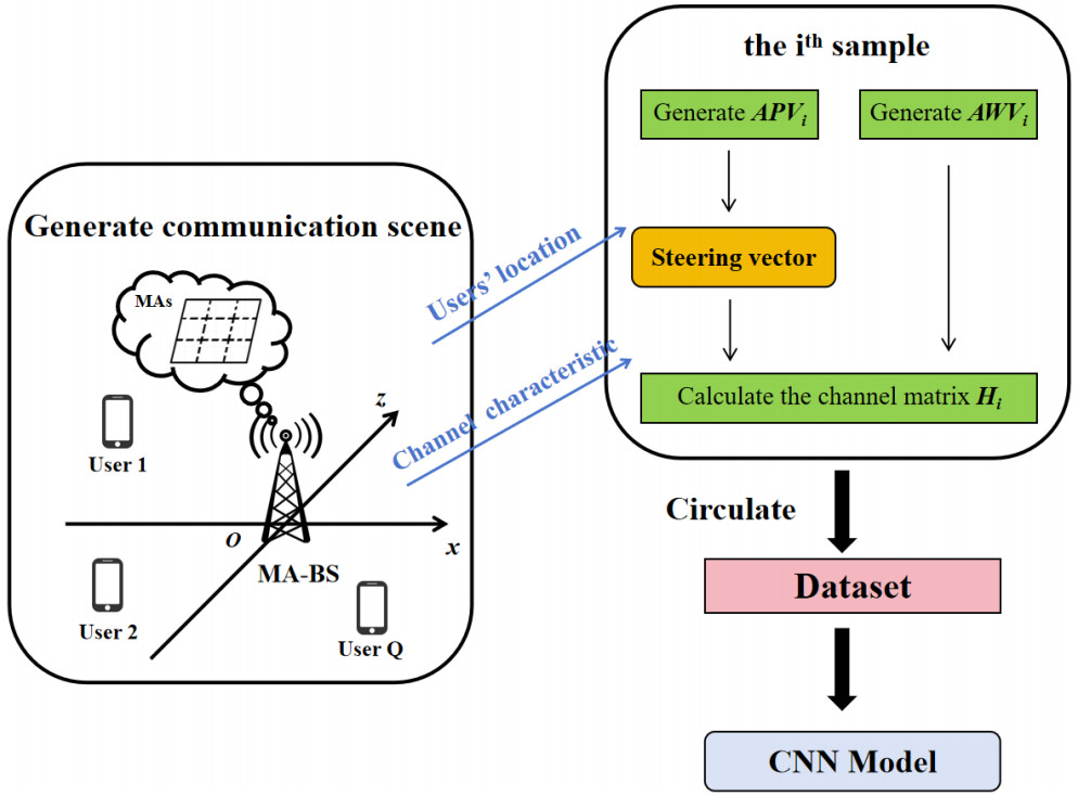
Figure 3. Demonstration of the proposed algorithm.

Several sets of antenna positions and antenna weights are randomly generated and the channel matrix under this configuration is computed as inputs and outputs, respectively, for the training of the network. The converged model outputs accurate channel matrices based on the randomness of the antenna positions and weights.

The datasets required for training and testing the model are generated. Each data consists of APV $$ \boldsymbol{p}_a \in C^{M \times 1} $$, AWV $$ \boldsymbol{w} \in C^{M \times 1} $$ and channel matrix $$ \boldsymbol{H}=[{\boldsymbol{g}}_1, {\boldsymbol{g}}_2, \dots, {\boldsymbol{g}}_Q]^T \in C^{Q \times M} $$. For each planar MA on the BS, since its position is randomly generated in its moving region, the $$ m $$-th antenna position $$ L(m) $$, $$ m \in \{1, 2, \dots, M\} $$, which is located in the $$ m_x $$-th row and $$ m_z $$-th column is formulated as^[28]:

and satisfies the constraint that the spacing between neighboring antennas is not less than $$ \Upsilon $$, given by^[28]:

where $$ \Upsilon $$ denotes the threshold value for the antenna spacing constraint. Note that the antenna location and constraint of the adjacent antenna spacing for the linear array are omitted for space saving. Setting $$ z_{m} = 0 $$ for all antennas yields the linear-array scenario, while retaining arbitrary $$ (x_{m}, z_{m}) $$ pairs corresponds to the planar array case. Furthermore, no separate derivations are required, and the subsequent optimization and CNN-based channel estimation method remain identical for both types of array structures.

The antenna positions satisfying the requirements are obtained and recorded, i.e., $$ \boldsymbol{p}_a = \{ L(1), L(2), ..., L(M) \} $$. In addition, a set of normalized AWV $$ \boldsymbol{w} $$ is randomly generated to adjust the signal weights of each antenna, which can be normalized as^[16]:

where $$ \parallel.\parallel_2 $$ represents the $$ L_2 $$ norm of a variable. Based on the antenna positions $$ \boldsymbol{p}_a $$, antenna weights w and users' position $$ \boldsymbol{p}_u $$, the channel matrix $$ \boldsymbol{H} $$ under the current conditions can be calculated. Afterwards, this set of data is organized and collected into the dataset, and the above process is looped for a new set of data generation until the number of dataset samples $$ {\bf{S}} $$ is reached.

When the dataset is obtained, the data preprocessing operation is performed. The data within the dataset is converted into CNN model input, and thus the training set and test set are divided. Afterwards, serving the channel matrix $$ \boldsymbol{H} $$ as the evaluation parameter for MSE computation, model training and evaluation are performed to allow this network to learn the relationship among APV $$ \boldsymbol{p}_a $$, AWV $$ \boldsymbol{w} $$ and channel matrix $$ \boldsymbol{H} $$, and each epoch's MSE and time consumption $$ T $$ are recorded. The formulation to minimize the MSE is given as^[21]

The framework of CNN-based approach for channel estimation in MA systems is summarized in Algorithm 1.

4. SIMULATION RESULTS

In this section, numerical results are provided to verify the effectiveness of the proposed method. Note that the unit for the size of MA movable region is set to $$ \lambda $$. Moreover, the minimum distance between adjacent MAs is defined as $$ \Upsilon=\frac{\lambda}{2} $$, and the number of training epochs is set to $$ 10 $$, with each batch consisting of $$ 32 $$ samples. The maximum distance between the user and the BS is $$ 500 $$ m, and the minimum distance between the user and the BS is $$ 50 $$ m. The transmit power and noise power from the BS are normalized to $$ 1 $$ W and $$ 1 $$ W, respectively, to focus on algorithmic differences rather than absolute Signal-to-Noise Ratio (SNR) levels. Standardization is considered to be the fulfillment of the maximum power limit of transmission; i.e., the maximum transmission power does not exceed $$ 100\% $$ of the system. The complex path gain is $$ {\alpha _{q, p}} \in (0, 1) $$. Furthermore, the training set in the dataset accounts for $$ 80\% $$, and the random seed is $$ 42 $$ to ensure the repeatability of the simulation.

To verify the advantages of the proposed method, benchmark schemes are established as control groups, including (1) LS-based method; (2) OMP-based method; (3) LR-based method. Selecting OMP as the benchmark for comparison due to the priority in research^[16], which has shown that flexible precoding based on OMP can more than double the rate in mobile antenna scenarios. In addition, the OMP method has advantages such as no offline training and interpretable results (sparse path gains directly correspond to physical propagation paths).

The computational complexity of our proposed algorithm is analyzed as follows. These expressions are derived analytically and validated by the measured runtime in the design results, i.e., CNNs: The network consists of two 1D convolution layers, and its floating-point operations (FLOPs) can be expressed as $$ O(M^{2}Q) $$; OMP: $$ O(P^{2}MQ) $$ per iteration with $$ P $$ paths. It is obvious that the system complexity increases linearly with respect to the variation of $$ Q $$.

Both linear and planar arrays are studied here to evaluate the effectiveness of antenna array design based on the MAs, and they move along the $$ x $$-axis and $$ x-z $$ axes for the linear and planar arrays, respectively. The number of antennas is $$ M = 32 \times 1 $$ and $$ M = {M_x} \times {M_z} = 8 \times 8=64 $$ for the linear and planar cases, respectively. Moreover, the corresponding numbers of samples $$ {\bf{S}} $$ of dataset are selected as $$ 2, 000 $$ and $$ 3, 000 $$ and the number of paths is selected as $$ P = 9 $$ for both of them.

Since the number of the users $$ Q $$ is selected from $$ \{ 2, 4, 6, 8, 10, 12, 14\} $$, the MSE of the channel matrix with respect to the number of users for various methods is displayed in Figure 4A and B for the linear and planar arrays, respectively. It is observed that although the difference of the measured MSEs between the OMP and CNN methods in several specified numbers of users can be ignored, the CNN-based method gives the lowest MSE among all methods. As illustrated in Figure 4A, the CNN captures spatial signatures with almost the same ease for a handful of users as for a dense population in the linear array scenario, while the greedy-based algorithm visibly struggles as more users enter the scene. The same performance is repeated in the planar case, as shown in Figure 4B, confirming that the additional $$ z $$-axis DoF does not disturb the network's ability to generalize; on the contrary, it offers extra spatial diversity that the CNN turns to its advantage. Overall, the proposed scheme avoids the error-floor that typically haunts iterative sparse-recovery approaches and thus offers a reassuring margin for future dense-cell deployments. It can be seen clearly that both CNN and OMP methods can achieve lower MSE than the other two methods, only the design results generated by the OMP and CNN methods are compared in the following parts.

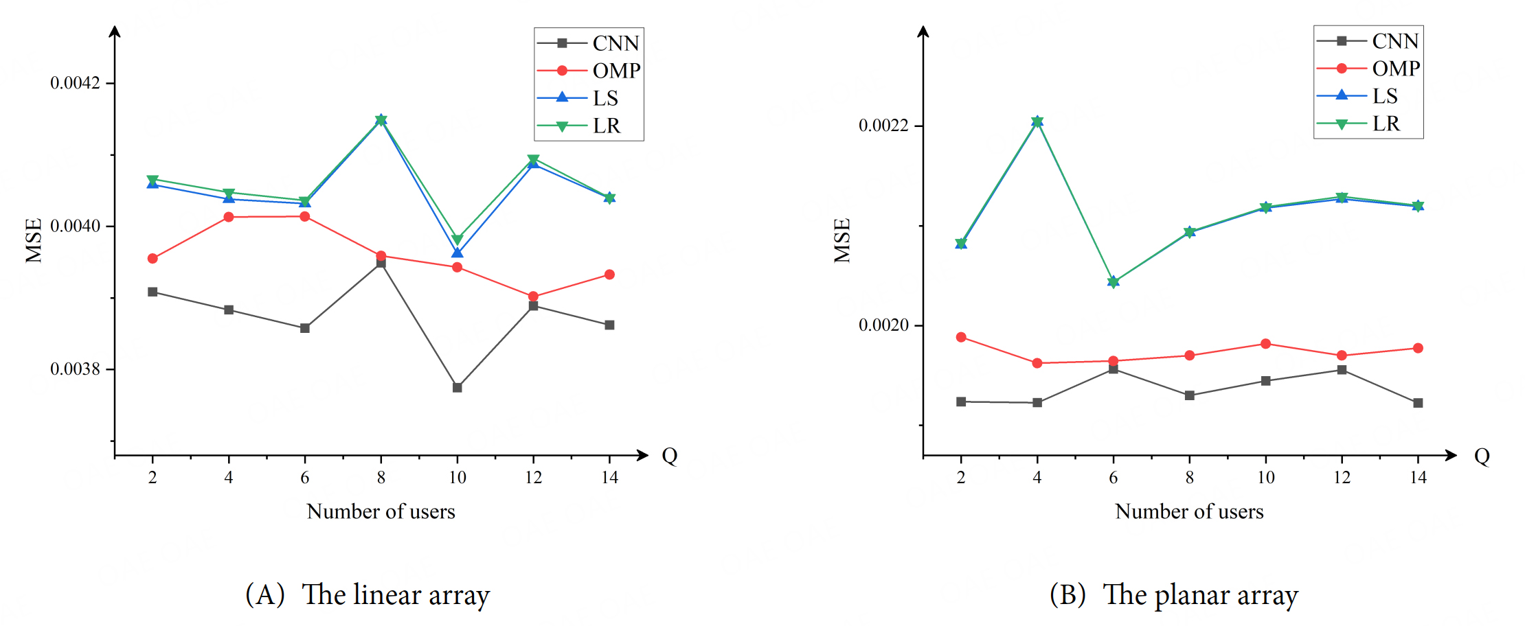
Figure 4. The MSE of channel matrix with respect to the number of users generated by the proposed method, OMP method, LS method and LR method: (A) The linear array; (B) The planar array. MSE: Mean square error; OMP: orthogonal matched pursuit; LS: least squares; LR: linear regression.

To further validate the robustness of training parameters, we conducted additional experiments. We fix the total number of samples of each training round at $$ 320 $$ and compared two network structure settings: epoch = $$ 10 $$, batch = $$ 32 $$ and epoch = $$ 16 $$, batch = $$ 20 $$. As shown in Figure 5, the results show that the MSEs for different schemes are nearly identical for both configurations, but the former had smaller gradient variance and a smoother convergence curve.

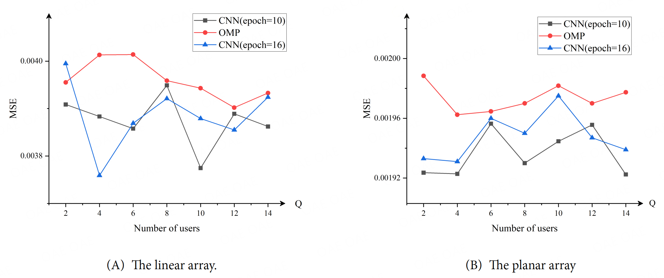
Figure 5. The MSE of channel matrix with respect to the number of users generated by the CNN method with epoch = 10, epoch = 16, and the OMP method: (A) The linear array; (B) The planar array. MSE: Mean square error; CNN: convolutional neural network; OMP: orthogonal matched pursuit.

Moreover, Figure 6 illustrates that more epochs only increase the computation time without yielding significant performance improvements, so we ultimately retain the configuration of epoch = $$ 10 $$ and batch = $$ 32 $$. With the increase of the number of users, the training convergence of time for the CNN model is guaranteed, but the time required by OMP method surges for different array structures, where Figure 6A and B is for the linear and planar arrays, respectively. As shown in Figure 6A, the linear panel shows that the CNN curves corresponding to the two training configurations lie almost on top of each other, indicating that the shorter-epoch schedule already yields sufficient accuracy. By contrast, the trace of the greedy algorithm bends visibly upward as more users enter the scene, reflecting the additional burden imposed by the iterative residual-cleaning loop. Figure 6B illustrates the same qualitative behavior in the planar case. The CNN curves remain overlapped regardless of epoch count, confirming that the additional $$ z $$-axis DoF does not increase training difficulty. Meanwhile, the OMP curve slopes more steeply, once again demonstrating that the lightweight network maintains an almost constant inference time even when the antenna population becomes dense.

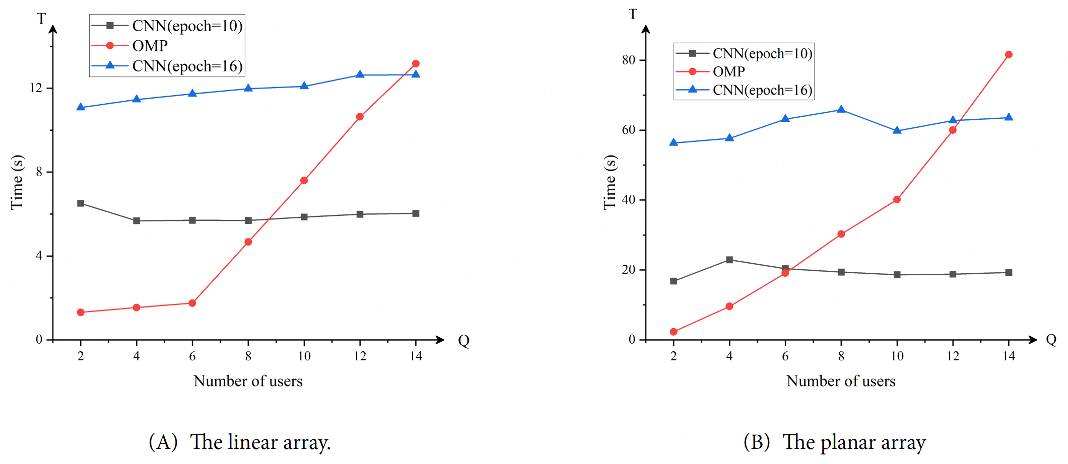
Figure 6. The consumed time with respect to the number of users generated by the CNN method with epoch = 10, epoch = 20, and OMP method: (A) The linear array; (B) The planar array. CNN: convolutional neural network; OMP: orthogonal matched pursuit.

When the number of users is not high, the consumed time with the OMP method is much shorter than that of the proposed method. With the increase of the dedicated users, the consumed time for OMP grows dramatically but the time for the proposed CNN network remains nearly unchanged. The CNN model processes the data in such a way that the convolutional kernels slide over the input data to perform the convolutional operation. When the number of users is increased, the properties and structure of the data do not change, and the number of convolutional kernels and parameters of the CNN model does not vary. Hence, the learnable parameters do not vary due to the rise in the number of users. Compared to the OMP method that gradually selects with the highest correlation coefficient to the residuals through an iterative algorithm, the CNN training convergence time is relatively constant and does not fluctuate significantly with respect to the increase in the number of users.

Although the CNN method exhibits slightly higher time consumption than OMP when the number of users is small (e.g., $$ Q $$ = 6), this trend changes significantly as $$ Q $$ increases. As shown in Figure 6, once $$ Q $$ exceeds 8, the time consumed by OMP rises sharply due to its iterative nature, while CNNs maintain a nearly constant inference time. This demonstrates that CNNs offer better scalability and efficiency in multi-user scenarios, which are more representative of practical communication systems.

The number of paths and the size of movable region of MA are also studied in this work. The numbers of users are $$ Q=6 $$ and $$ Q=8 $$ for the linear and planar arrays, and the numbers of samples in dataset are $$ 2, 000 $$ and $$ 3, 000 $$ for the linear and planar arrays, respectively. Moreover, the number of paths is selected from $$ \{3, 6, 9, 12, 15\} $$. The variation of MSEs of channel matrix generated by the OMP and the proposed method with respect to the number of paths is compared in Figure 7, where Figure 7A is plotted for the linear array case and Figure 7B is plotted for the planar array case. It can be seen that the proposed method gives the lower MSE values than the OMP method for nearly entire path range. In Figure 7A, CNNs show lower sensitivity to the number of paths because the convolutional kernels learn dominant angle clusters automatically due to their mechanism; In Figure 7B, a similar robustness is observed, confirming that the network extracts essential spatial features instead of relying on sparsity assumptions. Consequently, the proposed estimator is suitable for both sparse and rich-scattering environments without re-tuning, which simplifies field deployment.

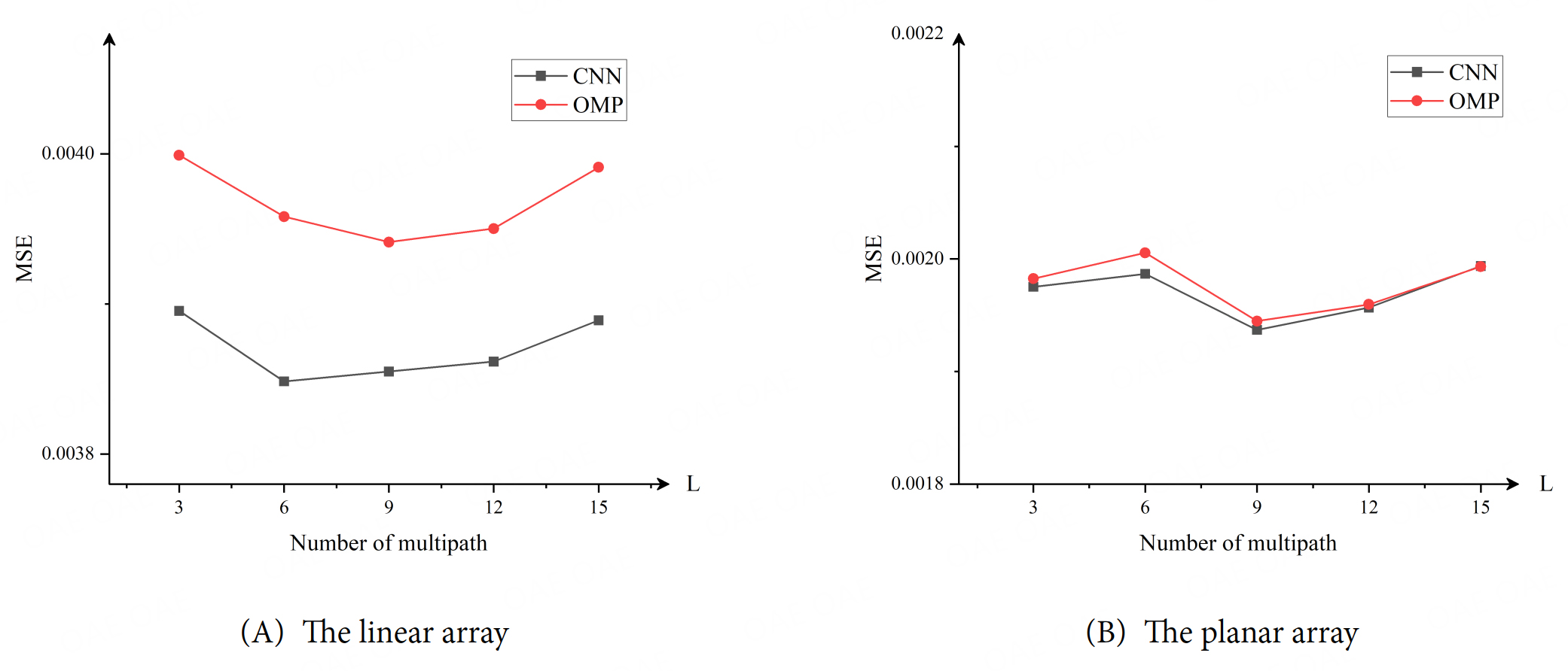
Figure 7. The MSE of channel matrix with respect to the number of multipaths generated by the proposed method and OMP method: (A) The linear array; (B) The planar array. MSE: Mean square error; OMP: orthogonal matched pursuit.

It is known that CNNs have high capability of powerful feature extraction, which is capable of learning complex features in the data. The OMP method performs channel estimation based on the sparsity of the signal, and in each iteration, OMP selects the optimum value based on the current residuals, and when the number of paths changes, the iterative process of OMP is still carried out in accordance with its convergence rules, and therefore is less sensitive to the changes in the number of paths, and similarly for the size of MA's movable region.

The size of the movable region for MA also affects the overall performance and it should be considered in this work. For the linear array, the number of users is $$ Q=6 $$ and the number of samples in dataset is $$ 2, 000 $$, and for the planar array, the number of users is $$ Q=8 $$ and the number of samples in dataset is $$ 3, 000 $$. The variation of MSEs with respect to the length of the moving region for the linear and planar arrays is displayed in Figure 8A and B, respectively. Except for several sampled points in the linear array, including $$ 5\lambda $$ and $$ 8\lambda $$, the proposed CNN network gives a lower MSE than the OMP method, and this behavior is similar to that observed in the planar array.

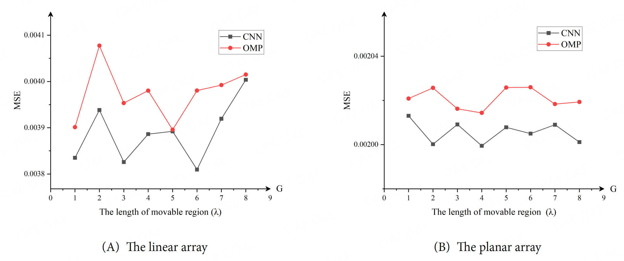
Figure 8. The MSE of channel matrix with respect to the length of each MA's movable region generated by the proposed method and OMP method: (A) The linear array; (B) The planar array. MSE: Mean square error; MA: movable antenna; OMP: orthogonal matched pursuit.

The essence of CNN's convolution operation is to identify the same features, i.e., while the size of MA's movable region changes, with respect to the spatial distribution of the channel, but the CNN focuses on extracting the essential features of the data. Thus, it is not sensitive to changes in the size of the movable region for MA.

To verify the efficiency and latency of this model, the variation of MSE with respect to the number of samples is investigated here. Using the MSE generated by the OMP method as a benchmark, Figure 9 illustrates that in both linear and planar arrays the MSE from the OMP method is lower than that of the CNN network when the number of sample points is low. However, the proposed CNN method can deal with the problem better when the number of samples is high in both types of arrays. As illustrated in Figure 9A, CNN outperforms OMP once samples exceed 200 in linear case, indicating that the network benefits from data-driven generalization; OMP accuracy saturates because it is model-based. As shown in Figure 9B, a similar crossing point is observed in the planar scenario, but more samples are required than in the linear case to achieve the same accuracy. This confirms that the convolutional approach is convergent when measurement campaigns are affordable and indicates that the minimum number of samples needed to achieve satisfactory accuracy while avoiding excessive overhead.

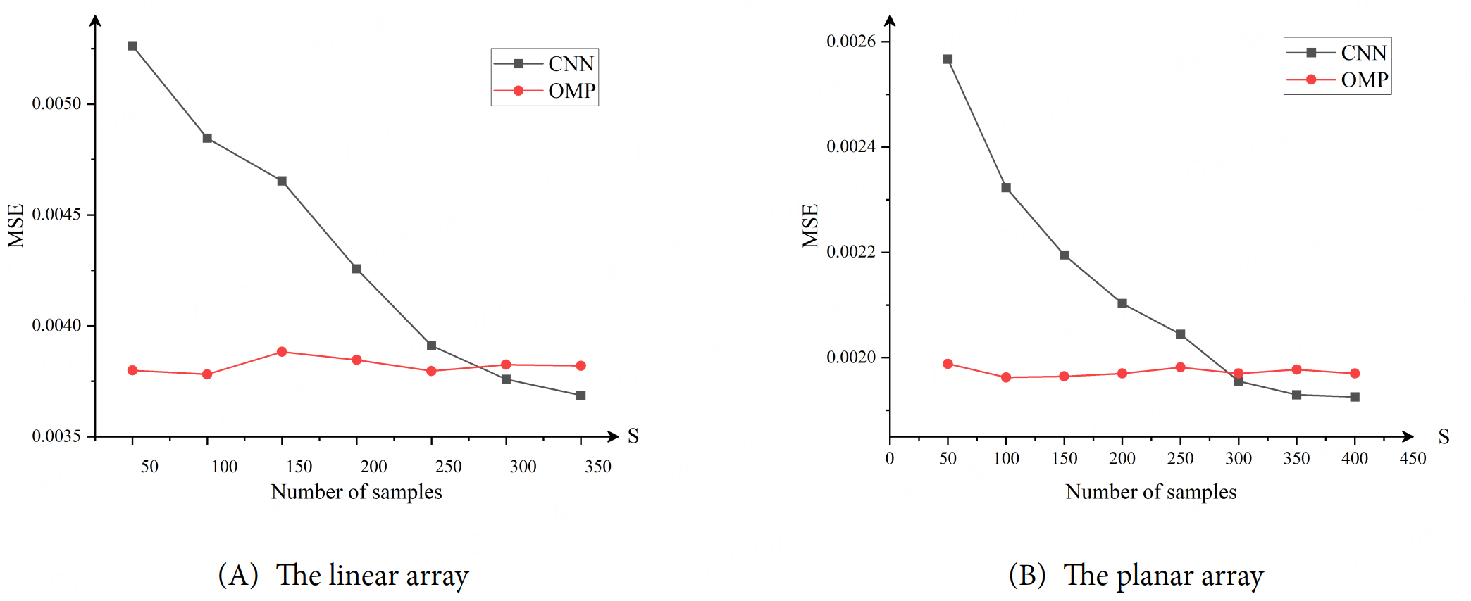
Figure 9. The MSE of channel matrix with respect to the number of the samples generated by the proposed method and OMP method: (A) The linear array; (B) The planar array. MSE: Mean square error; OMP: orthogonal matched pursuit.

Overall, the relationship between the convergence time and the number of samples can directly reflect the efficiency of the model to learn the data features because the computational resources are limited and expensive when actually training the model. Determining the minimum number of samples to meet the model performance requirements can not only avoid employing too many samples for training and increasing the data volume, but also reduce the overhead of computational resources, which is suitable for application scenarios with high real-time requirements.

5. CONCLUSIONS

Based on the inspiration of DL algorithms, a CNN-based channel estimation method is proposed for the configuration of BS that is equipped with MA arrays to deal with the complex problem of multi-data, multi-users and large computational volume. Compared with the LS method, OMP method and LR method, the proposed method not only realizes satisfactory channel estimation from the perspective of MSE, but also effectively employs the shortest computational time in a multi-user communication scenario. Design results verify the superiority of the proposed method compared to other approaches and the proposed method provides a good solution for the application of MA in real wireless communication systems.

DECLARATIONS

REFERENCES

1. Han, S.; Liao, Y.; Chen, S.; Liang, Y. C. Joint channel estimation for RIS-aided mmWave MIMO wireless communication systems with mixed-resolution quantization schemes. IEEE. Internet. Things. J. 2025, 12, 33756-68.
2. Lu, S.; Liu, F.; Li, Y.; Zhang, K.; Huang, H.; Zou, J. Integrated sensing and communications: recent advances and ten open challenges. IEEE. Internet. Things. J. 2022, 11, 19094-120.
3. Cheng, Q.; Zhang, L.; Dai, J. Y.; Tang, W.; Ke, J. C.; Liu, S. Reconfigurable intelligent surfaces: simplified-architecture transmitters - from theory to implementations. Proc. IEEE. 2022, 110, 1266-89.
4. Kang, J. M. Deep learning enabled multicast beamforming with movable antenna array. IEEE. Wireless. Commun. Lett. 2024, 13, 1848-52.
5. He, C.; Lu, Y.; Chen, W.; Ai, B.; Wong, K. K.; Niyato, D. Graph neural network enabled fluid antenna systems: a two-stage approach. IEEE Trans. Veh. Technol. 2025. https://discovery.ucl.ac.uk/id/eprint/10209042/1/Graph_Neural_Network_Enabled_Fluid_Antenna_Systems_A_Two-Stage_Approach.pdf. (accessed 20 Oct 2025).
6. Chen, Y.; Chen, M.; Xu, H.; Yang, Z.; Wong, K. K.; Zhang, Z. Joint beamforming and antenna design for near-field fluid antenna system. IEEE. Wireless. Commun. Lett. 2025, 14, 415-9.
7. Ma, W.; Zhu, L.; Zhang, R. Multi-beam forming with movable-antenna array. IEEE. Commun. Lett. 2024, 28, 697-701.
8. Zhu, L.; Ma, W.; Zhang, R. Modeling and performance analysis for movable antenna enabled wireless communications. IEEE. Trans. Wireless. Commun. 2024, 23, 6234-50.
9. Ye, Y.; You, L.; Wang, J.; Xu, H.; Wong, K. K.; Gao, X. Fluid antenna-assisted MIMO transmission exploiting statistical CSI. IEEE. Commun. Lett. 2024, 28, 223-7.
10. Ma, W.; Zhu, L.; Zhang, R. MIMO capacity characterization for movable antenna systems. IEEE. Trans. Wireless. Commun. 2024, 23, 3392-407.
11. Zhu, L.; Ma, W.; Ning, B.; Zhang, R. Movable-antenna enhanced multiuser communication via antenna position optimization. IEEE. Trans. Wireless. Commun. 2024, 23, 7214-29.
12. Zhu, L.; Ma, W.; Zhang, R. Movable-antenna array enhanced beamforming: achieving full array gain with null steering. IEEE. Commun. Lett. 2023, 27, 3340-4.
13. Hu, G.; Wu, Q.; Ouyang, J.; Xu, K.; Cai, Y.; Al-Dhahir, N. Movable-antenna-array-enabled communications with CoMP reception. IEEE. Commun. Lett. 2024, 28, 947-51.
14. Li, N.; Wu, P.; Ning, B.; Zhu, L. Sum rate maximization for movable antenna enabled uplink NOMA. IEEE. Wireless. Commun. Lett. 2024, 13, 2140-4.
15. Xiao, Z.; Pi, X.; Zhu, L.; Xia, X. G.; Zhang, R. Multiuser communications with movable-antenna base station: joint antenna positioning, receive combining, and power control. IEEE. Trans. Wireless. Commun. 2024, 23, 19744-59.
16. Yang, S.; Lyu, W.; Ning, B.; Zhang, Z.; Yuen, C. Flexible precoding for multi-user movable antenna communications. IEEE. Wireless. Commun. Lett. 2024, 13, 1404-8.
17. Tang, J.; Pan, C.; Zhang, Y.; Ren, H.; Wang, K. Secure MIMO communication relying on movable antennas. IEEE. Wireless. Commun. Lett. 2025, 73, 2159-75.
18. Qin, H.; Chen, W.; Li, Z.; Wu, Q.; Cheng, N.; Chen, F. Antenna positioning and beamforming design for fluid antenna-assisted multi-user downlink communications. IEEE. Wireless. Commun. Lett. 2024, 13, 1073-7.
19. Hu, G.; Wu, Q.; Xu, K.; et al. Fluid antennas-enabled multiuser uplink: a low-complexity gradient descent for total transmit power minimization. IEEE. Commun. Lett. 2024, 28, 602-6.
20. Wang, C.; Li, Z.; Wong, K. K.; Murch, R.; Chae, C. B.; Jin, S. AI-empowered fluid antenna systems: opportunities, challenges, and future directions. IEEE. Wireless. Commun. 2024, 31, 34-41.
21. Jang, S.; Lee, C. New view of learning-aided channel estimation for movable antenna systems. IEEE. Trans. Wireless. Commun. 2025, 24, 5694-708.
22. Tang, X.; Jiang, Y.; Liu, J.; Du, Q.; Niyato, D.; Han, Z. Deep learning-assisted jamming mitigation with movable antenna array. IEEE. Trans. Veh. Technol. 2025, 74, 14865-70.
23. Weng, C.; Chen, Y.; Zhu, L.; Wang, Y. Learning-based joint beamforming and antenna movement design for movable antenna systems. IEEE. Wireless. Commun. Lett. 2024, 13, 2120-4.
24. Fadakar, A.; Mansourian, A.; Akhavan, S. Localization using convolutional neural networks with mobile array. In 2024 IEEE 100th Vehicular Technology Conference (VTC2024-Fall), Washington, USA. October 07-10, 2024. IEEE; 2024. p. 1-5.
25. Mamamed, A.; Bai, Z.; Femi-Philips, O.; et al. Low complexity deep neural network based transmit antenna selection and signal detection in SM-MIMO system. Digit. Signal. Process. 2022, 130, 103708.
26. Tsakiris, M. C.; Peng, L.; Conca, A.; Kneip, L.; Shi, Y.; Choi, H. An algebraic-geometric approach for linear regression without correspondences. IEEE. Trans. Inf. Theory. 2020, 66, 5130-44.
27. Zhang, J.; Liu, W.; Gu, C.; Gao, S. S.; Luo, Q. Multi-beam multiplexing design for arbitrary directions based on the interleaved subarray architecture. IEEE. Trans. Veh. Technol. 2020, 69, 11220-32.
28. Xie, C.; Xiu, Y.; Yang, S.; Zhang, Z. Deep learning for movable antenna precoding in 2D MISO communication system. In 2024 10th International Conference on Computer and Communications (ICCC), Chengdu, China. December 13-16, 2024. IEEE; 2024. pp. 2500-4.
29. Zheng, Q.; Saponara, S.; Tian, X.; Yu, Z.; Elhanashi, A.; Yu, R. A real-time constellation image classification method of wireless communication signals based on the lightweight network MobileViT. Cogn. Neurodyn. 2024, 18, 659-71.
30. Zheng, Q.; Tian, X.; Yu, Z.; et al. MobileRaT: a lightweight radio transformer method for automatic modulation classification in drone communication systems. Drones 2023, 7, 596.
31. Zheng, Q.; Tian, X.; Yu, L.; Elhanashi, A.; Saponara, S. Recent advances in automatic modulation classification technology: methods, results, and prospects. Int. J. Intell. Syst. 2025.
Cite This Article
How to Cite
Download Citation
Export Citation File:
Type of Import
Tips on Downloading Citation
Citation Manager File Format
Direct Import: When the Direct Import option is selected (the default state), a dialogue box will give you the option to Save or Open the downloaded citation data. Choosing Open will either launch your citation manager or give you a choice of applications with which to use the metadata. The Save option saves the file locally for later use.
Indirect Import: When the Indirect Import option is selected, the metadata is displayed and may be copied and pasted as needed.
About This Article
Special Topic
Copyright
Data & Comments
Data
0
Comments
Comments must be written in English. Spam, offensive content, impersonation, and private information will not be permitted. If any comment is reported and identified as inappropriate content by OAE staff, the comment will be removed without notice. If you have any queries or need any help, please contact us at [email protected].