

A method for quantifying the upfront carbon footprint of urban densification in Texas through 2050
 0

Graphical Abstract
Abstract
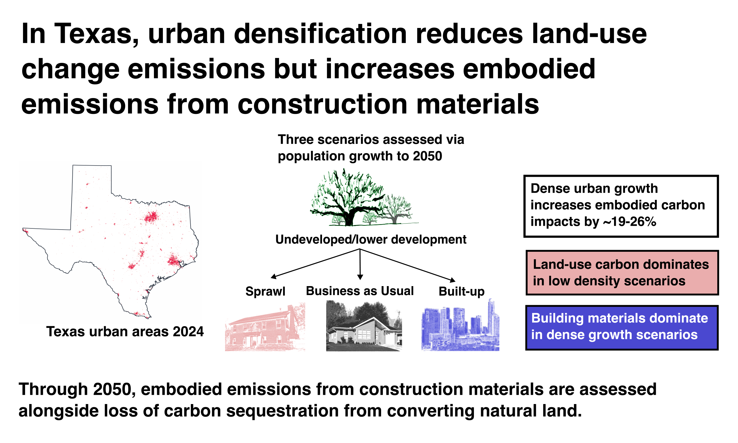
Urbanization is a major contributor to greenhouse gas emissions, and the Intergovernmental Panel on Climate Change projects that urban areas may grow by up to 211% globally by 2050. Embodied emissions make up a considerable portion of the total carbon footprint of urban areas. This study explores the relationship between urban densification and its upfront carbon footprint in Texas through 2050, using a novel method that combines land cover change projections, building stock analysis, and carbon sequestration quantification. Three densification trajectories–Sprawl, Business as Usual, and Built-Up–were used to demonstrate the method's ability to quantify upfront carbon footprint for a range of plausible urbanization outcomes. The analysis found that embodied emissions from building materials made up 71% of the upfront carbon footprint in Built-Up scenarios but only 40% in Sprawl scenarios, where lost carbon sequestration from the conversion of fields and forests to buildings and roads was the most significant factor. The central finding of this study is that high levels of urban densification lead to a larger upfront carbon footprint. Dense urban cores reduce natural land conversion but at the expense of increased emissions from the construction materials required for vertical development. Therefore, urban densification comes with a tradeoff between land-carbon effects and embodied emissions from buildings that should be taken into account in development of urbanization policy. Importantly, that same densification might lead to substantial avoided carbon emissions from more efficient operation and reduced transportation distances, but operational analysis was beyond the scope of this study.
Keywords


 Download PDF
INTRODUCTION
Background and motivation
Anthropogenic greenhouse gas emissions have substantial negative impacts on the climate, ecosystems, and human health[1,2]. The 2015 Paris Climate Summit called for mobilization of multiple stakeholders, including cities, in pursuing ambitious mitigation goals[3]. However, the buildings and construction sector, which constitutes the majority of the built environment's impacts, is not on track for Paris-aligned decarbonization goals[4].
Cities make up just 3% of global land area, but they account for 60%-80% of energy consumption and 75% of carbon emissions[5]. Today, about 55% of the world's population resides in cities, but the United Nations reports that this value could increase to 68% by 2050[6]. Increasing urban populations could expand global built area by as much as 211% in that same time period[7].
Buildings themselves account for 32% of global energy use and 34% of CO2 emissions from operational and embodied sources[4], and these figures make buildings the highest single contributing sector to emissions. To reach Net Zero scenario goals, the energy intensity of the buildings sector needs to decrease nearly five times as fast over the next decade as it has in the past decade[8].
Total building emissions are quantified as the sum of operational and embodied emissions. Embodied emissions of buildings—indirect emissions sources such as manufacturing and transportation of materials—accounted for an estimated 12.95% of global emissions in 2022[8]. Literature suggests that embodied emissions for individual buildings can make up anywhere between 20%-90% of life cycle building emissions, depending on the operational efficiency of the building[9,10], and it can take decades for that cost to be offset by in-use efficiencies, even in sustainable buildings[7]. These emissions are directly tied to each building's construction materials, type, height, and floor area. In 2024, global building floor area increased 1.7% on the previous year to reach 273 billion m2 (square meters)[11], and this upward trend is expected to continue in parallel to increased urbanization. Awareness that embodied emissions of buildings are comparable to operational emissions has only recently emerged[12,13], and as such the United Nations has called for a more wholistic, life-cycle approach to be taken in the evaluation of a building's impact[14].
This study takes a land-use focused approach to estimating the impact of buildings on overall carbon emissions. Most literature that seeks to quantify the carbon footprint of urban development fails to account for the loss of natural/agricultural land due to urban expansion, despite the Global Carbon Budget's finding that land-use change emissions were approximately 4.2 GtCO2 (billion metric tons of CO2) in 2024, or about 10% of total anthropogenic CO2 emissions[15]. Quesada et al. found that the inclusion of Land Use/Land Cover Change (LULCC) enhances projections of carbon loss from land disturbances by about 49%[16]. Urbanization contributes heavily to these land disturbances[17], and it has a much longer lasting impact than other types of land cover change[18]. To provide a more integrated assessment, this study links land-cover change, building embodied emissions, and land-carbon impacts to evaluate the upfront carbon footprint of urbanization. We define the upfront carbon footprint as the sum of three components—embodied emissions of building materials, carbon-stock losses from land conversion, and foregone future sequestration—recognizing that this extends the conventional supply-chain meaning of "embodied" to include land-based carbon effects.
Urban expansion is often complex and heterogeneous. Some cities tend towards more dense, tall urban centers to keep up with growing population, while others sprawl outwards in more suburban and exurban archetypes. Urban density can reduce some forms of per-capita emissions and land consumption[19,20], but it can also shift development toward different building forms, materials, and consumption patterns[21]. Many studies find that urban densification is correlated with lower emissions because of more efficient building operation, access to transit options, and shorter transportation distances for commuting and daily life[22,23,20]. There are exceptions to this conventional wisdom, including Chen et al., who suggest that when direct and indirect emissions are taken into account, total household emissions increase significantly from rural to urban living[24].
Conversely, cities with shorter buildings and wider sprawl convert much more natural land to built environment, thereby losing significantly more natural carbon stocks. Since upfront carbon footprint is affected by urban densification, and exact urban expansion pathways are difficult to predict, modeling a range of urban densification scenarios is imperative for projecting realistic carbon footprint effects of urbanization. Ribeiro et al. emphasize that modeling emissions based solely on scaling population growth or urban density neglects the strong interplay between the two factors and can result in a significant modeling error[25]. This study seeks to bridge that gap by creating a model driven by population growth in tandem with broad urban densification scenarios. It should be noted that a well-developed, parallel body of literature considers land-use change in relation to transportation systems[26,27], and another body of literature examines operational emissions from the built environment[7], but neither transportation land-use changes nor operational emissions are the focus of this study.
This paper quantifies the upfront carbon footprint of urban development in the U.S. state of Texas from the present through 2050 for a range of population growth and urban densification scenarios. Texas provides a high-impact case study for urban carbon-footprint analysis because it combines rapid population growth, large projected development pressure, and a major emissions profile. The Texas Demographic Center (TDC) projects that the state's population could grow from approximately 32 million in 2026 to 42 million in 2050[28]. Additionally, in 2025 the Texas GDP reached $2.9 trillion (or 9.4% of U.S. GDP), and it continues to grow[29]. Not only is Texas primed for massive urban expansion from population and GDP growth, but it also produced approximately 727.96 MtCO2e (million tonnes of CO2-equivalent) of greenhouse gas (GHG) emissions in 2022, approximately 12% of U.S. and 1.6% of global emissions[30,31]. Texas is therefore a useful test case for the interplay between urbanization and emissions.
Research question
This study seeks to answer the following question: At the state level, how does the urban densification in Texas affect the upfront carbon footprint associated with urbanization?
Using a combination of LULCC techniques, building stock analysis, and carbon sequestration quantification, this model establishes nine upfront carbon footprint scenarios of urban development in Texas through 2050. These scenarios include three population growth pathways (Low, Mid, and High) combined with three densification trajectories (Sprawl, Business as Usual (BAU), and Built-Up). The expectation is that comparison of these scenarios will yield valuable insight into urban densification's effects on upfront carbon footprint, which has potential to inform emissions-reducing policy and play a part in addressing climate change at large. This methodology is demonstrated in Texas but transferrable to other states or regions where data are available and can be used on a broader scale to understand how best to develop policy to help meet emissions goals.
Other studies, such as Zhang et al.' s 2024 land use simulation of Ezhou, China, use comparable LULCC modeling and scenario techniques to project built-up land use change[32]. However, to the authors' knowledge, no other study has developed the specific LULCC methodology presented here nor conducted a state-wide analysis and projection of Texas's urban upfront carbon footprint.
METHODS
Study scope and scenario design
This study develops and deploys a model to discover whether urban densification affects the upfront carbon footprint of Texas through 2050. Upfront carbon footprint is defined as the sum of embodied emissions of future building stock, the loss of carbon sequestration stocks through development of natural land to make way for those new buildings, and foregone future sequestration. To measure the effects of urban densification, three density scenarios were projected and analyzed: Sprawl, BAU, and Built-up. These scenarios represent a wide, but reasonable, range of possible outcomes and are described in depth in Section "Density scenario implementation". Comparison of the respective upfront carbon footprint of each of these density scenarios shows how urban densification has an effect and allows the development of policy to mitigate the impacts of expected urbanization on total carbon emissions. It is not expected that the effects of urbanization on upfront carbon impact will compare in magnitude with its influence on the carbon impact of operational energy and transportation; however, such upfront carbon effects are as yet unexplored in Texas and should be quantified to gain a more holistic picture of the total life-cycle carbon impact of built environment expansion.
To assess the cumulative upfront carbon impact of urbanization, the model uses a combination of remotely-sensed land data, cellular automata (CA) projections, and historical building and population trends. The backbone of the model uses population projections from the TDC[28] to drive LULCC projections at 30 m resolution for 16 developed and natural land use archetypes at 5-year intervals, to 2050. Projected land cover changes are then used directly to inform loss of natural carbon sequestration stocks through each evaluation period. To quantify the embodied emissions effects of new buildings, 2021 per capita building stock values are attached to population and LULCC projections to estimate new buildings for each period. Future building stock projections are paired with emissions intensity values derived from the literature to obtain total embodied emissions. Taken together, carbon sequestration losses and embodied building emissions projections paint a clear picture of the effects of urban densification and what components drive those effects. A flow diagram outlining this general methodology is shown in Figure 1.
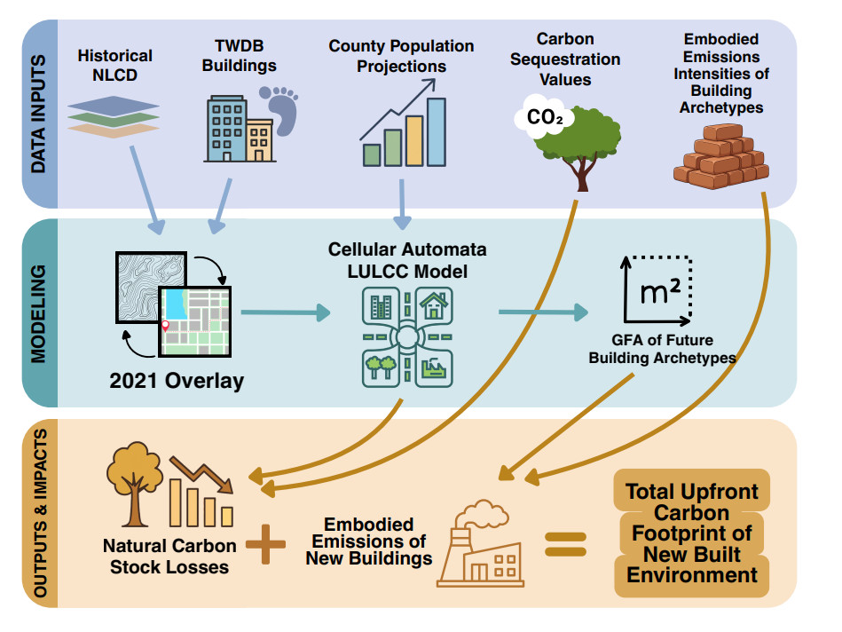
Figure 1. Flow diagram of overall methodology used in this study. national land cover database (NLCD) land cover[33], TWDB buildings[34], and TDC population datasets[28] are combined to produce a novel LULCC model that informs calculation of embodied carbon footprint of the Texas built environment. The diagram was created using Canva, and all icons and graphical elements are from Canva's built-in content library. https://www.canva.com/.
While this approach is robust for depicting overall trends at a large scale, the model has practical limitations at higher spatial resolutions. LULCC projections are reliant on multiple remotely-sensed datasets, each of which contains underlying error. Published estimates of carbon sequestration rates, carbon stocks, and embodied emissions intensities vary across studies, therefore representative coefficients were synthesized from multiple literature sources and applied consistently across scenarios. In spite of these potential limitations, due to the fact that our main goal is to compare different scenarios using the same model and same assumptions, the results are directionally instructive for understanding the relative impacts of different domains of embodied carbon.
Data sources and preprocessing
Analysis of the upfront carbon footprint associated with Texas urbanization began with obtaining, cleaning, and validating high-quality datasets. Many building stock analyses employ survey data, such as the U.S.-based Residential Energy Consumption Survey, but this model primarily uses empirical data obtained through remote sensing[19,35]. This approach provides a level of detail not available through tax records or other formal records of building sizes, which might underestimate total footprints[36]. Three datasets formed the basis of this work, and they are described below. In addition, urban emissions intensity and carbon sequestration coefficients were collected from literature and are displayed below. Collectively, these datasets provided a framework for the creation of density scenarios and a CA LULCC tool that can be used to analyze the effects of urban densification on Texas' upfront carbon footprint.
The United States geological survey (USGS) national land cover database (NLCD)
USGS NLCD provides annual raster data for the United States at 30 m resolution, classified into twelve natural and four developed land-use archetypes[33]. The 2021 NLCD layer was processed and clipped to Texas to establish baseline empirical relationships between land use, buildings, and population. 2021 data was used because the latest corresponding buildings and population datasets are from that time period [Figure 2]. Developed categories are defined by percent imperviousness: open space (OS), 1%-19%; low intensity (LI), 20%-49%; medium intensity (MI), 50%-79%; and high intensity (HI), 80%-100%. Percent imperviousness refers to the fraction of a given area covered by surfaces that prevent or substantially reduce water infiltration, such as roads, rooftops, and parking lots. Interestingly, the processed 2021 NLCD layer showed that most of the imperviousness in Texas exists within the "Texas Triangle, " the area broadly outlined by Dallas-Fort Worth, San Antonio, and Houston [Figure 2]. Due to the coarseness of NLCD resolution, many known rural buildings are misinterpreted as natural land. As such, for buildings-related projections in this study, all natural land use archetypes (0% imperviousness) are combined into one Non-developed (ND) category. Descriptions of representative housing types for each developed category are provided in Supplementary Table 1.
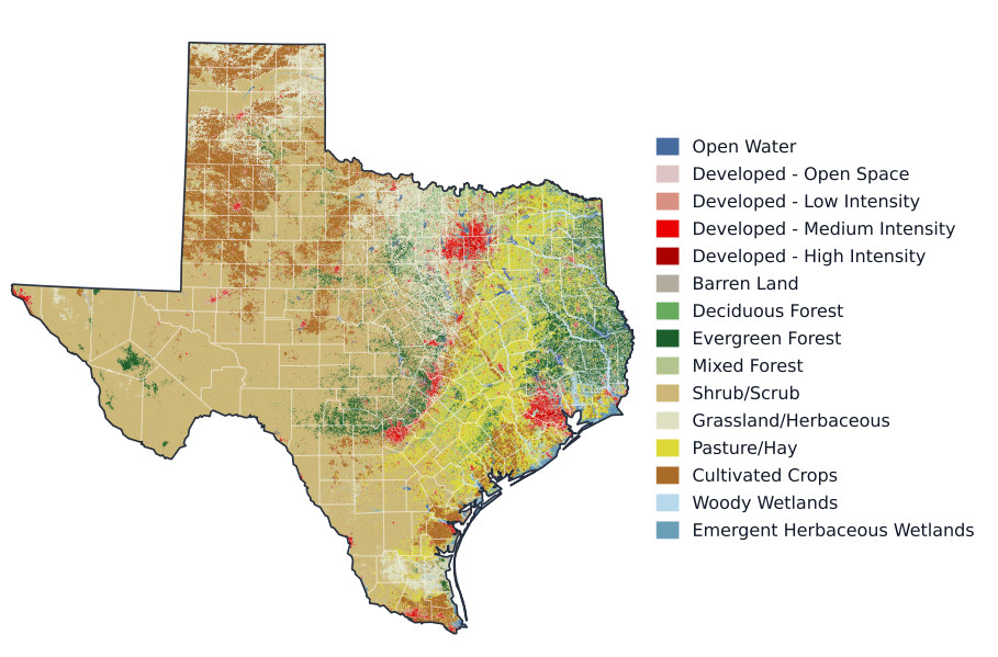
Figure 2. 2021 National Land Cover Database map clipped to Texas–used to develop baseline empirical relationships between land use, buildings, and population that feed the land cover change projections. Red pixels indicate urban settings, and it is clear that most of the current built environment exists within the "Texas Triangle"–the area broadly outlined by Dallas-Fort Worth, San Antonio, and Houston. Projections are driven by population growth and take place at the county level, which are outlined in white. County boundaries from Esri (2014)[37]; Texas state outline derived from the county polygons.
Annual NLCD data were used instead of legacy NLCD products because the annual collection provides a methodologically consistent basis for analyzing historical land-cover change. NLCD data have been widely used in LULCC and urbanization studies[38,39]. Validation of the Annual NLCD Collection indicates a thematic accuracy, how correctly land-use types are identified, of approximately 79%, supported by a modernized deep-learning framework for annual land-cover and impervious-surface monitoring[33,40,41].
2021 Texas Water Development Board (TWDB) buildings dataset
TWDB provides a multi-faceted, Texas-wide buildings dataset that includes estimates for each building of: footprint, building type, day/night population, building height, and gross floor area (GFA)[34]. The approximately 10.9 million building footprints were developed by the Texas Geographic Information Office from a combination of Microsoft Artificial Intelligence Version 2, Open Street Map (July 2021 version), and light detection and ranging (LiDAR) building footprints from 2010 to 2019[42]. The dataset defines six building types: Agricultural, Commercial, Industrial, Public, Residential, and Vacant/Unknown. Validation checks of the dataset revealed limited errors in total floor values impacting a small number of buildings in San Angelo, which were incorrectly labeled as having 120 stories, which is taller than Texas's tallest building. These estimates were removed and treated as missing and were part of the approximately 27% of buildings lacking height data due to incomplete LiDAR coverage and other data errors. Because height is critical for estimating GFA and embodied energy, missing values were imputed using the median height of buildings within the same type and footprint-size decile, derived from the 73% of buildings with known heights. It should also be noted that approximately 0.02% of the population was lost in the night population estimate. Additionally, an indicative analysis of the TWDB dataset in comparison to cadastral data (see the Sensitivity and Uncertainty Analysis section of the Supplementary Materials) found some potential bias in gross floor area estimations derived from the TWDB dataset. Despite these limitations, the TWDB database is among the richest available dataset on Texas buildings.
TDC population growth pathways
County-level population projections were obtained from the TDC Vintage 2024 Population Projections[28]. Three population growth scenarios—low, mid, and high—are defined in this dataset, informed by the U.S. Census Bureau's national projection series. The projections are given in 10-year increments through 2060 and include data-driven estimates of mortality, fertility, and migration. For this research, the projections were clipped to 2050, and 5-year intervals were interpolated. Visualization of these pathways at the state level can be seen in Supplementary Figure 1. Projection assumptions and migration scenarios were interpreted using TDC's accompanying methodology report[43].
Embodied emissions intensity coefficients for buildings
In this study, embodied emissions are defined using a cradle-to-gate boundary, including life-cycle modules A1-A3: raw material supply, transport to manufacturing, and product manufacturing. Construction, use-stage replacement, end-of-life, and later stages are excluded. Embodied emissions coefficients were developed from literature for low-rise, mid-rise, and high-rise buildings for each building type defined in the TWDB buildings dataset and are provided in Supplementary Table 2. Embodied emissions coefficients used in this model range from 0.1-0.6 tCO2e m-2 (metric tons of CO2-equivalent per square meter) and are variably affected by building height. A more in-depth discussion of the methodology used to obtain these coefficients is provided in the Supplementary Materials.
Carbon sequestration coefficients
For this model, aboveground vegetation carbon stock (tC ha-1) (metric tons of carbon per hectare), soil carbon stock (tC ha-1), and aboveground carbon sequestration rate (tC ha-1 yr-1) (metric tons of carbon per hectare per year) were approximated. Coefficients were assigned by land-cover class using values synthesized from published literature. Final values and supporting sources are provided in Supplementary Table 3.
Baseline empirical relationships
This study quantifies the upfront carbon footprint of Texas urban development through 2050 using historical data and scenario-based projection techniques. The framework is driven by a novel overlay of 2021 land cover, building stock, and population data used to derive empirical baseline relationships. Based on this overlay, county-level imperviousness was found to be well described by a linear function of county-level population density [Figure 3]. Therefore, imperviousness was used as a measurable proxy for population density. NLCD data are already organized by five levels of imperviousness, as described in Section "The United States geological survey NLCD", so category names were retained: HI, MI, LI, OS, and ND. These development categories serve as proxies for different tiers of population and urban density.
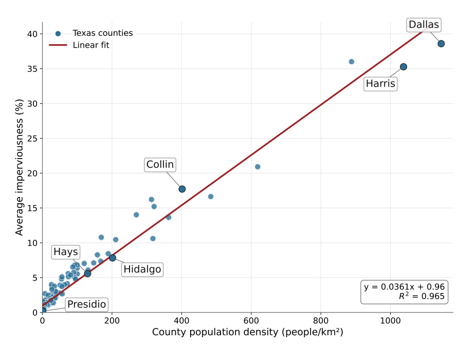
Figure 3. 2021 County Average Imperviousness as a function of population density. Imperviousness increases consistently with population density, furthering the notion that population drives built environment development. As such, imperviousness is used as a proxy for population and urban density in this model. Labeled counties were selected to give a relative understanding for what different levels of population density and imperviousness look like. Dallas and Harris counties represent the urban cores of the Dallas–Fort Worth and Houston metropolitan areas, respectively. Collin, Hidalgo, and Hays counties represent different levels of suburban and exurban land cover, and are located in the DFW, Rio Grande Valley, and San Antonio areas, respectively. Presidio County is located in rural West Texas.
For each development category, population allocation share, defined as the percentage of county population residing in that category, and category population density were plotted as functions of total county population density. As shown in Supplementary Figure 2, fitted log-linear piecewise functions were mapped onto the empirical relationships and used to estimate population allocation share and category population density for future counties based on projected total population density. The methodology for defining Sprawl and Built-Up scenarios is explained in Section "Density scenario implementation". In addition, the 2021 overlay provides reference building statistics for each development category, including GFA and floor area per capita (FAC), which inform the building stock projection model.
As shown in Figure 4, residential FAC decreases with increasing urban density. This inverse relationship is consistent with prior findings by Güneralp et al.[20]. In contrast, FAC for commercial, industrial, and public buildings is extremely low in every developed category except High-Intensity. Despite the observation that average dwelling size decreases with increased urban density, the total amount of floor space attributable to each person grows significantly in response to urban densification. For all numerical values underlying Figure 4, see Supplementary Table 4.
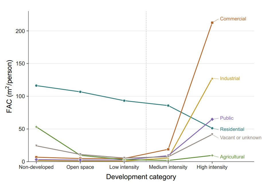
Figure 4. 2021 Texas Floor Area per Capita (FAC) for each building type across NLCD development categories. Residential FAC decreases with development intensity, while commercial, industrial, and public FAC increase sharply in high-intensity developed areas. Numerical values, including total FAC by development category, are provided in Supplementary Table 4.
Land-use/land-cover projection model
Once baseline empirical relationships were established between land cover and population, a LULCC projection tool was developed that mimics NLCD land use archetypes. This tool is driven by county level TDC population projections and starts by allocating new developed land to each county. At each 5-year time step, total predicted county population density is calculated. Using population/land cover relationships derived from the 2021 overlay (see Supplementary Figure 2), category population allocation share and population density are derived. Population allocation share defines the percentage of new population assigned to each development category, and category population density translates the assigned population into new land.
New developed land within each county was allocated using a CA framework constrained by statewide source-class shares derived from observed 2000–2024 land-cover transitions [Supplementary Table 5]. A fixed source-class distribution was applied separately to each developed land-cover category. Within these source quotas, eligible pixels were ranked based on neighborhood effects and subject to a binary exclusion mask[44]. Tied suitability scores were resolved randomly, and unmet source quotas spilled over to other eligible source classes. Pixels were transitioned until the required new land area for each development category was allocated. Land cover projections were seeded with observed 2024 NLCD data as their starting point. An example of the LULCC projections for the Mid-BAU scenario is shown in Figure 5 of Hays county: observed 2024 and projected 2050. With this modeling framework, developed land coverage in Hays County increases from 18.22% to 36.37%. Hays County was selected as a representative fast-growing corridor county because it contains expanding urban and suburban development while retaining substantial non-developed land. The comparison illustrates how the model allocates projected growth across existing developed areas, urban edges, and previously undeveloped land-cover classes.
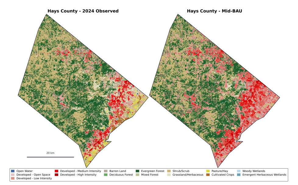
Figure 5. Example LULCC projection for Hays County, Texas, comparing observed 2024 land cover with projected 2050 land cover under the Mid-BAU scenario. With this modeling framework, developed land coverage in Hays County increases from 18.22% to 36.37%. Hays County was selected as a representative fast-growing corridor county because it contains expanding urban and suburban development while retaining substantial non-developed land. The comparison illustrates how the model allocates projected growth across existing developed areas, urban edges, and previously undeveloped land-cover classes. Hays County boundary from Esri (2014)[37].
Many widely used LULCC and urban-growth modeling frameworks require detailed socioeconomic, behavioral, parcel-level, transportation, or exclusion-layer data that can be difficult to assemble consistently across large study areas[45,46,47]. In contrast, this model uses a smaller set of broadly available inputs: historical NLCD land-cover data, population density, and county-level population projections. This simpler model is more reproducible at state or national scales while retaining sufficient spatial structure for comparative scenario analysis. The LULCC model was validated using a similar technique to Zhang et al.[32] : the model was calibrated with NLCD data from 1985–2000, then land use change was projected from 2000–2024 using the calibrated model parameters and driven by historical county population data. For 2000–2024, the model achieved a Figure of Merit of 0.17, which is in the range of values reported for established land-change models[48].
Density scenario implementation
To explore the effects of densification, the model produced land use change and building stock projections for nine different scenarios – three density scenarios at three potential population growth pathways. The three population growth pathways (low, mid, and high) are given by county and are obtained directly from the TDC. The three density scenarios are defined as: Sprawl, BAU, and Built-Up. The sprawl scenario corresponds to a general shift towards less urban densification and more rural dwelling, as compared to BAU. The Built-Up scenario corresponds to increased urban densification and more city dwelling. Scenario names are shown in Table 1.
Scenario naming convention for population-growth and densification scenarios
| Densification scenario | |||
| Population-growth scenario | Sprawl | BAU | Built-Up |
| Low | Low-Sprawl | Low-BAU | Low-Built-Up |
| Mid | Mid-Sprawl | Mid-BAU | Mid-Built-Up |
| High | High-Sprawl | High-BAU | High-Built-Up |
To create the Sprawl and Built-Up density scenarios, new projected population within each county was synthetically shifted towards higher or lower imperviousness as compared to BAU. As explained in Section "Land-use/land-cover projection model", county-level population allocation directly influences urban land development. As shown in Supplementary Figure 2, BAU piecewise population allocation share functions were modified to simulate increased or decreased urban densification. For Sprawl and Built-Up scenarios, the functions were shifted to 90th and 10th percentiles for each development category as presented in Table 2. The choice of these percentiles reflects values towards the upper and lower ends of plausible futures.
Density scenario adjustment factors applied to population allocation across land-use categories
| Density scenario | Non-developed | Open space | Low intensity | Medium intensity | High intensity |
| Sprawl | 90th | 90th | 90th | 10th | 10th |
| BAU | - | - | - | - | - |
| Built-Up | 10th | 10th | 10th | 90th | 90th |
Additional details on the land-use/land-cover change projection workflow, spatial allocation procedure, transition weights, suitability constraints, and land-carbon accounting assumptions are provided in the Supplementary Methods.
Upfront carbon impact accounting
Embodied emissions from buildings
To assess future embodied emissions of Texas buildings, models of future building stock were created for each scenario by combining 2021 building stock per capita values from Figure 4 with population projections. Informed by that synthesis, GFA projections were generated for each development category, building type, and building height category. Projected GFA was converted to embodied GHG emissions using building-type-specific emissions intensities found in Supplementary Table 2. This stock-level approach is consistent with archetype-based embodied carbon modeling, where representative building types are assigned embodied carbon intensities and scaled to the broader building stock[49]. Because higher-density scenarios accommodate the same population within a smaller building footprint, one might expect per-capita embodied carbon to differ from these aggregate totals. However, within each population-growth pathway, all three density scenarios share the same total population, so a per-capita normalization scales every scenario identically and leaves the relative differences between scenarios unchanged.
Carbon stock losses
Once development was projected using the LULCC tool, initial carbon stock losses for the transition from natural to developed land for each period and scenario were estimated using carbon emissions coefficients unique to each ND category, as shown in Supplementary Table 3. For each natural land-use archetype, carbon stocks were calculated for both soil and aboveground vegetation. Sequestered carbon of aboveground vegetation was assumed to be entirely released to the atmosphere, while soil organic carbon (SOC) stocks were considered to release only 30% of their carbon stocks upon disturbance from development. This generalized value is synthesized from a combination of literature sources[50,51], since the fraction released depends on the specific land-use transition and soil depth, and in general there is a large amount of uncertainty and limited data in this field of study[52]. Because soil-carbon loss scales with land conversion, this parameter affects land-intensive scenarios (Sprawl) more than compact ones (Built-Up); nonetheless, varying the SOC loss fraction from 15% to 45% preserved the ranking of scenarios, with the relative differences between them changing by less than 10% [Supplementary Table 6]. To minimize error while maintaining focus on the effects of urban development, intra-category land-use transition for the Non-Developed development category was prohibited in the LULCC calculator. Therefore, potential re-forestation and afforestation efforts are unaccounted for in this study.
In addition to direct losses of accumulated carbon sequestration, our model estimated the reduction in potential future carbon sequestration due to loss of natural land to development. Our study refers to this lost carbon sequestration potential as foregone carbon sequestration. Trees and plants continue to sequester carbon as they age and grow, but urban development of natural land stifles any growth opportunities. Only aboveground carbon sequestration rates were included in this projection, as literature is unclear on the carbon accumulation rate of soil.
Cumulative upfront carbon impact
The upfront carbon footprint of Texas urbanization is defined in this study as the sum of embodied emissions of new buildings, lost natural carbon stocks, and foregone natural carbon sequestration. For each scenario, cumulative upfront carbon footprint is quantified at each time-step from 2030–2050. Because higher-density scenarios accommodate the same population within a smaller building footprint, one might expect per-capita upfront carbon impact to differ from these aggregate totals. However, within each population-growth pathway, all three density scenarios share the same total population, so a per-capita normalization scales every scenario identically and leaves the relative differences between scenarios unchanged.
Key assumptions and limitations
The model designed for this study produces land cover change and upfront carbon footprint projections that are robust at the aggregate, state-level, but certain assumptions and limitations reduce their effectiveness at higher spatial resolution. First, the 30 m NLCD resolution is coarse enough that neighborhood-scale development transitions are low-fidelity. Additionally, the four broad divisions of developed land defined by NLCD lose some detail and granularity. However, due to the sheer size of land area modeled—Texas covers some 268, 596 square miles—and the systems-level reporting adopted, these limitations were deemed acceptable.
Another potential limitation to this work is that the TWDB buildings dataset remains unvalidated at the individual building level, due to its size (~10.9 million buildings). However, low-rise residential buildings account for approximately 78% of buildings in the processed TWDB dataset, which is consistent with external housing-stock summaries showing that single-family residential units dominate Texas housing[53]. Because this dominant category is assigned a consistent embodied emissions intensity statewide, isolated building-type or height classification errors are unlikely to substantially alter aggregate embodied emissions trends. Absent a radical improvement in building codes with respect to carbon intensity or dramatic improvements in building materials carbon efficiency, it is expected that these intensities will hold for the duration of the time period under consideration.
In addition, the model is limited to the embodied carbon footprint of buildings. In-use and transportation emissions play large roles in overall carbon footprint and are expected to be significantly affected by urban densification. However, the goal of this study is to isolate the impact of static, embodied emissions. Further work should be done to gain a more holistic view of how urban densification affects Texas' carbon footprint.
Finally, this model excludes the possibility of infill development, where existing infrastructure and developed land is used to place new population. Excluding infill development could overestimate the amount of developed land needed to house the same population. This limitation is driven by the lack of a reliable, time-varying buildings dataset for Texas. The 2000-2024 backcast using historical population data revealed an overestimation of 30.4% when comparing the projected 2024 developed land area to actual 2024 NLCD data. Higher fidelity projections will only be possible with temporally explicit buildings datasets.
The robustness of the scenario rankings results found in Section "RESULTS AND DISCUSSION" with relation to key input parameters—including embodied emissions coefficients and soil carbon release fraction—is assessed in the sensitivity analysis section of the Supplementary Materials [Supplementary Tables 6 and 7]. The relative differences between scenarios within each population growth pathway are preserved across all tested ranges.
Together, these methods define a population growth-driven cellular CA for projecting land-cover change in Texas through 2050. The resulting land-use projections are used to estimate embodied emissions from new building stock, natural carbon stock reductions, and foregone carbon sequestration across the nine scenarios.
RESULTS AND DISCUSSION
Quantifying the total upfront carbon impact of the three different density scenarios (Sprawl, BAU, and Built-Up) gives direct insight into whether urban densification will have an impact on the carbon footprint of Texas. While the findings in this research—embodied emissions of the building stock and loss of natural carbon sequestration—only represent pieces of the puzzle (for example, as noted before, operational emissions are not included in this analysis), they define key factors that contribute to urban densification's carbon footprint.
Urban densification leads to a higher upfront carbon footprint
As shown in Figure 6, the Built-Up density scenario produces the highest cumulative upfront carbon impact within each population growth pathway, followed by Sprawl, then BAU. Built-Up scenarios show upfront carbon impact values around 22% higher than Sprawl scenarios and 30% higher than BAU scenarios (see Supplementary Table 8). This result suggests that urban densification carries a larger upfront carbon footprint cost than other pathways for accommodating future population growth in Texas. The results indicate that the relative influence of each factor—embodied emissions from new buildings, initial land carbon loss, and foregone carbon sequestration due to the loss of carbon-fixing land-types—varies across scenarios.
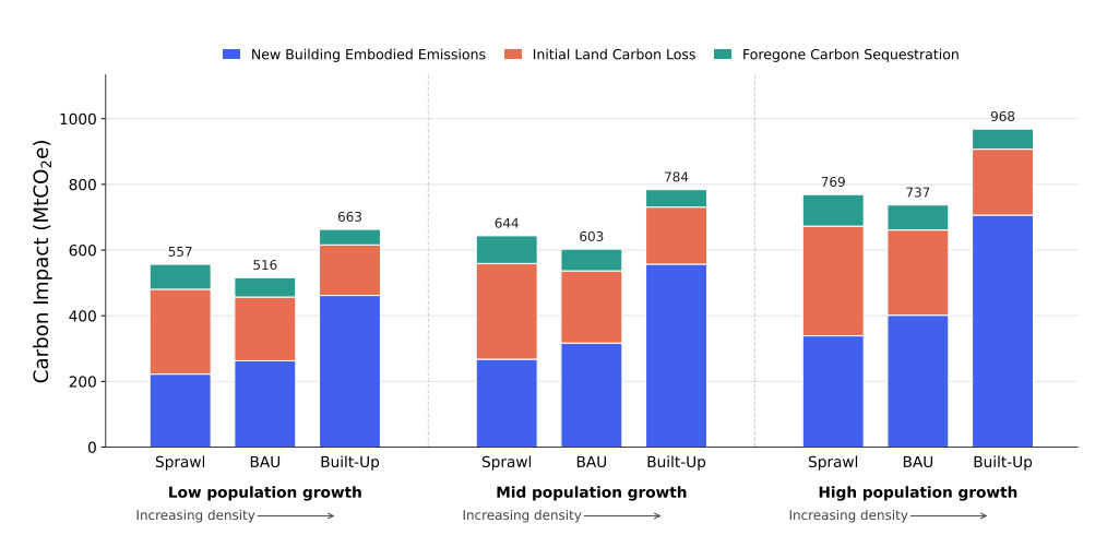
Figure 6. Cumulative upfront carbon impact of all nine scenarios by 2050. Upfront carbon footprint is largest in Built-Up scenarios, showing that while dense urban cores use less land for new buildings, the extra materials required for this densification offset the gains achieved through more efficient use of land. Upfront carbon footprint in Sprawl scenarios is conversely much more affected by loss of natural land and associated carbon stocks. Values are rounded; see Supplementary Table 8 for full precision.
The most significant cumulative contributor to upfront carbon footprint is embodied buildings emissions, followed by initial natural land carbon loss, then foregone carbon sequestration. However, with decreasing urban densification carbon sequestration impacts start to become more comparable to buildings effects. In the Low-Sprawl and Mid-Sprawl scenarios, Initial Land Carbon Loss accounts for a larger share of total upfront carbon impact than New Building Embodied Emissions, by 6.5 and 3.7 percentage points, respectively. Additionally, because initial carbon losses and foregone carbon sequestration are inherently coupled, it is instructive to compare their sum with embodied building emissions. In all Sprawl scenarios, initial carbon losses plus foregone carbon sequestration amount to more than new building embodied emissions.
Increased urban densification is directly correlated with increased GFA of the statewide building stock. In the Built-Up scenario, more tall buildings are constructed in less space, and the resulting increase in gross floor area amounts to more embodied building emissions. Conversely, decreased urban densification (Sprawl scenario) results in the development of more natural land, which directly impacts loss of carbon sequestration. The BAU scenario produces the lowest cumulative upfront carbon footprint due to medium effects from both buildings and loss of natural land.
Additionally, upfront carbon impact effects scale proportionally with population growth, which is expected because the model is inherently driven by population growth projections. As shown in Figure 7, the model projects that upfront carbon footprint effects will rise steadily through 2050 for every scenario, which is consistent with Friedlingstein et al. and their claim that total anthropogenic CO2 emissions are on the rise year to year[15].
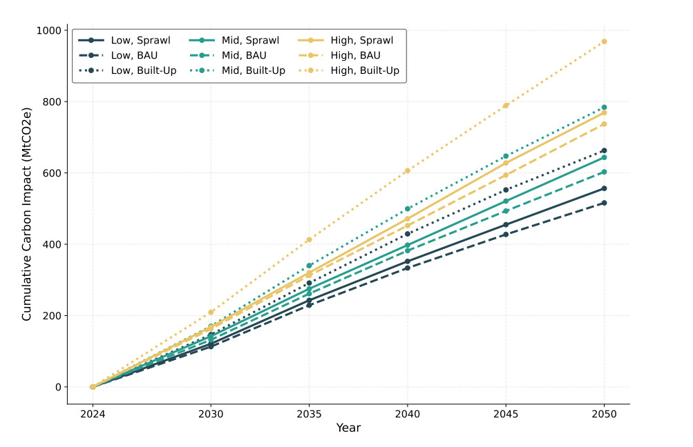
Figure 7. Cumulative upfront carbon impact of all nine scenarios through 2050. Carbon impacts scale proportionally with population growth and are expected to grow through 2050. The average annual carbon impact across all projected scenarios is 26.67 MtCO2e/yr, which is less than 4% of the 2022 Texas GHG emissions total of 727.96 MtCO2e[30].
Annual total upfront carbon impact from the built environment only makes up a small percentage of Texas' total annual GHG emissions. The Greenhouse Gas Inventory for Texas reports 727.96 MtCO2e in total GHG emissions for 2022[30]. This model projects average annual upfront carbon impact values of 21.41–29.57 MtCO2e/yr for Sprawl scenarios, 19.84–28.35 MtCO2e/yr for BAU scenarios, and 25.49-37.25 MtCO2e/yr for Built-Up scenarios, depending on the population growth pathway. These values represent approximately 3%-5% of total annual Texas GHG emissions, which is lower than global averages for the percent of total GHG emissions attributed to embodied emissions from the built environment[11]. This difference is likely due to the much higher contribution of electric power generation and transportation in Texas. For example, in 2024, the Energy Information Administration reported that Texas CO2 emissions were 185.0 MtCO2 for the electric power sector and 227.4 MtCO2 for the transportation sector[54,55], which is substantially higher than the annualized embodied emissions from even the most impactful scenario (High-Built-Up). Intentional patterns of built-environment growth can have long-term effects that extend well beyond initial embodied and land-carbon impacts. By shaping infrastructure, land-use patterns, and everyday travel behavior, development decisions can either lock in high-emissions trajectories or support lower operational and transportation emissions over time.
The following sections explore the individual contributions of each upfront carbon footprint factor.
Effects from embodied building emissions increase with urban densification
At high levels of urban densification (i.e., Built-Up scenarios), embodied building emissions make up approximately 71% of the cumulative upfront carbon footprint. As explained in Section "Embodied eissions intensity coefficients for buildings", embodied building emissions in this study includes raw material supply, transport to manufacturing, and product manufacturing. This model calculates embodied emissions from buildings as a function of building floor area, with individual emissions intensity coefficients for each building type and height envelope (see Supplementary Table 2). Figure 8 shows a breakdown of embodied emissions contributions by building type, for each scenario.
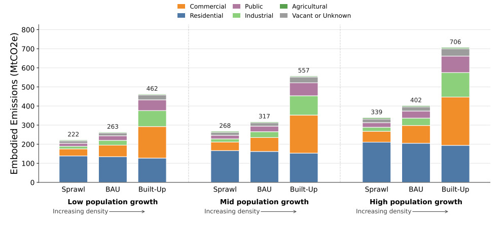
Figure 8. Total cumulative embodied emissions of projected Texas building stock through 2050. Although residential FAC decreases with increasing density, residential embodied emissions remain relatively similar across scenarios because denser residential development shifts more floor area into taller, multi-family buildings with higher embodied emissions intensities. In Built-Up scenarios, commercial, industrial, and public buildings account for a larger share of total embodied emissions, consistent with literature suggesting that higher-density urban environments can be associated with greater non-residential activity and consumption-related demand. Values are rounded; see Supplementary Table 9 for full precision.
Figure 8 shows that contributions from Residential buildings decrease slightly with increased urban densification, and for BAU and Sprawl scenarios they make up more than half of the total embodied emissions. With increased urban densification, more of the population lives in high-density cities, which is associated with smaller residential FAC. Residential embodied emissions remain similar across density scenarios because lower residential FAC in Built-Up scenarios is partially offset by a shift toward taller, multi-family residential buildings, which are assigned higher embodied emissions intensities. This finding is consistent with prior research showing that, in the United States, multifamily buildings can have embodied emissions per square meter that are five to ten times higher than those of single-family detached homes[49].
Additionally, embodied emissions from commercial, industrial, and public buildings rise significantly with increasing urban densification. Effects from commercial buildings alone see an approximately 340% increase in nominal embodied emissions from Sprawl to Built-Up scenarios within each population growth pathway (see Supplementary Table 9). This analysis shows that urban living is associated with much more total FAC across all building types. People in cities have easier access to more commercial, industrial, and public amenities, and in addition these buildings tend to be taller than in more rural areas. Both of these factors contribute to high embodied emissions from buildings in Built-Up scenarios. These results are supported by findings from Gill et al. that urban living is associated with far higher consumer and leisure activity than rural living[21].
These results should not be interpreted as an inherent carbon penalty of densification, but rather as a consequence of the building-type and embodied emissions assumptions used in this scenario framework. Prior work has identified timber and other low-carbon structural systems as potential pathways for reducing the embodied emissions of taller buildings, with engineered timber assemblies capable of substituting for some steel and reinforced-concrete applications while also storing biogenic carbon[56,57]. Additionally, more than half of the state and national residential building stock was built in the 1980s. Many of these buildings are therefore are reaching the end of their plausible lifetime of around 50 years, which provides a unique opportunity for emissions-reduction policy in embodied carbon over the next 10 years to mitigate effects of this expected turnover[49]. Furthermore, the operational-energy and transportation emission reductions associated with urban densification are substantial[20,23] but were not included in this analysis, which focused on the embodied aspects only. A full accounting of the net climate effect of densification would require integrating these operational savings against the embodied penalty identified here.
Carbon stock loss increases with sprawl
The upfront impact of natural carbon stock losses scales with sprawl. Moving from Built-Up to {BAU} to Sprawl scenarios, the model allocates a progressively larger share of population growth and new developed land to previously undeveloped natural land-cover classes. More development of natural land results in more loss of carbon stock to the atmosphere, whether that be from the conversion of grassland, farmland, or forest.
As shown in Figure 9, grassland, pasture, shrubland, and evergreen forest land type conversions have the biggest carbon stock impacts, but for a variety of reasons. Supplementary Figure 3 shows that, depending on the scenario, evergreen forests make up only 6%-8% of converted natural area (see Supplementary Table 10), but their overall carbon impact is substantially higher due to high carbon stock coefficients (see Supplementary Table 3). Conversely, grassland, pasture, and shrubland all have extremely low carbon stock coefficients, yet their share of carbon impact is substantial because of their large shares of converted natural land. As scenarios tend more towards Sprawl, the share of lost carbon stocks from forested lands, combining all three forest types, approximately doubles because urbanization expands past easier-to-access grasslands and pastures that are in the close periphery of metro centers. Specific primary forest protection policy would mitigate some of this effect, even under a sprawl scenario. Additional biodiversity benefits of such protections are not quantified in this paper, but are substantial.
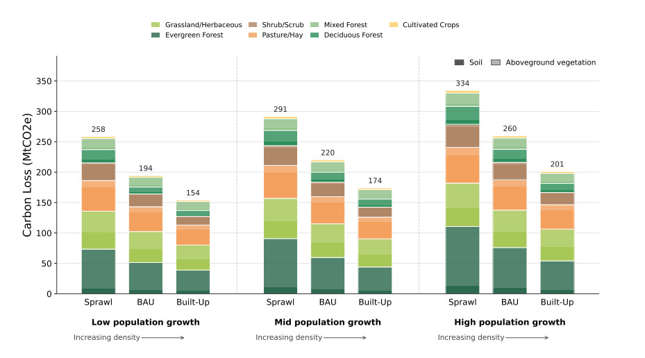
Figure 9. Carbon stock loss through 2050 by scenario and natural land type. Values represent the amount of sequestered CO2 that will be removed upon development of different types of natural land. Contributions from aboveground vegetation vs. soil are shaded light and dark, respectively. Carbon stock losses decrease approximately linearly with increasing urban density, since land is used more efficiently in scenarios with higher urban densification. Soil carbon-stock loss accounts for approximately 41%-44% of total carbon-stock loss, depending on the scenario. Values are rounded; see Supplementary Table 11 for full precision.
As explained in Section "Carbon stock losses", carbon stock loss is defined as the sum of aboveground vegetation carbon stocks and 30% of soil carbon stocks. In Figure 9 aboveground stocks are shown in a lighter shade, while soil stocks are shown in a darker shade for each land-use category. While soil carbon stocks house a significant portion of worldwide terrestrial carbon[58], literature suggests that soil disturbance due to development only releases approximately 30% of the soil carbon stocks to the atmosphere[59]. This 30% is a loss factor applied to the original soil stock, rather than the expected soil share of total modeled carbon loss. Because the soil carbon reservoir on converted land is larger than the corresponding aboveground reservoir, soil losses account for approximately 41%-44% of the combined carbon stock loss across the modeled scenarios.
While other types of land-use conversion (i.e. forest to cropland) induce significant reduction in global carbon stock, the effects of urbanization are likely to be longer-lasting and more difficult to reverse[18]. Zhang et al. suggest that urban forests have approximately 27% of the carbon sequestration capability of natural forests covering the same land area[60]. While an important step for mitigation, efforts to replace natural forests after development cannot be viewed as a one-to-one replacement of natural forests.
Overall, the loss of natural carbon stocks through land use conversion is a major factor in quantifying urban carbon footprint. However, as suggested by Quesada et al, many carbon emissions studies do not account for LULCC and therefore overestimate carbon sequestration potential[16].
Foregone carbon sequestration plays a consistent role in cumulative upfront carbon impact
As shown in Figure 6, foregone carbon sequestration makes up a small, but effectual, portion of the overall upfront carbon impact (6%-14%). Foregone carbon sequestration represents the cumulative carbon that would have been sequestered by natural land if it had remained undeveloped, but is no longer captured after conversion to developed land. Figure 10 outlines the breakdown of foregone sequestration potential by land-use archetype.
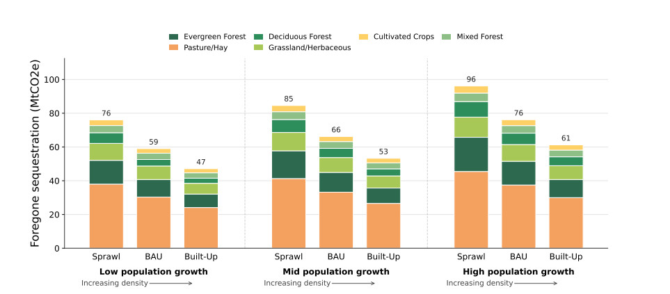
Figure 10. Foregone potential for carbon sequestration through 2050 by scenario and natural land type. Aggregate values represent the predicted accumulation of sequestered CO2 if no new natural land was converted into developed land. Foregone carbon sequestration decreases proportional to increasing urban densification as less natural land is developed and more carbon stock sites continue to sequester carbon. While still significant in the long term, foregone potential for carbon sequestration only makes up approximately 6%-14% of the total built environment upfront carbon impact through 2050. Values are rounded; see Supplementary Table 12 for full precision.
As shown in Figure 10, formerly pastured lands have the highest share of foregone carbon sequestration potential for all nine scenarios. The range of carbon sequestration rates across all natural land categories is small (0.3-2.6 tC ha-1 yr-1; see Supplementary Table 3); therefore, foregone carbon sequestration is heavily influenced by the nominal area of each category converted into developed land. As shown in Supplementary Figure 3, pasture/hay and grassland/herbaceous have the two highest amounts of total land conversion and correlate to two of the three highest contributors to foregone carbon sequestration.
Upfront carbon impact will cluster around existing metro hubs
As shown in Figure 11 (representing the Mid-BAU Scenario), cumulative upfront carbon impact through 2050 will be largely concentrated around existing metro hubs in the central, eastern section of the state. This area, broadly outlined by Dallas/Fort Worth, San Antonio, and Houston, is colloquially termed the "Texas Triangle". The Texas Triangle is host to about 75% of the state's population, much of its arable land, and 73% of its GDP[29]. It should be noted that the land-carbon effects modeled in this study occur on-site through vegetation and soil carbon changes, whereas building embodied emissions are largely indirect impacts associated with off-site material extraction, manufacturing, transportation, and construction supply chains. Because these emissions are less visible at the point of final building use, they may be more difficult for residents and decision-makers to perceive than local land-cover changes[12,13].
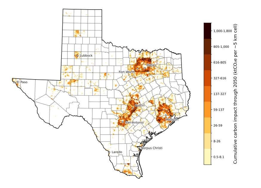
Figure 11. Cumulative upfront carbon impact of the projected Texas building stock growth for the BAU scenario and Mid population growth pathway from 2024 to 2050, using the methodology described in this study. The vast majority of upfront emissions are projected to occur within the highly populous "Texas Triangle" segment of the state. While the loss of carbon sequestration is felt and seen directly by residents and stakeholders, embodied building emissions are harder to visualize, as they are incurred largely indirectly and off-site of the end use. County boundaries from Esri (2014)[37]; Texas state outline derived from the county polygons.
A close inspection of the major cities reveals that very little additional upfront carbon footprint is attributed to the actual city centers, primarily because those areas are already at the highest intensity of urban densification, and our model framework does not allow for increased densification within these areas. In an examination of Texas urban development from 2001-2016, Guo et al. support this finding with the discovery that expansion of high urban intensity in the Texas Triangle occurred primarily in the periphery of major cities[61]. However, recent policy changes in 2023 and 2024 that reduced minimum lot sizes in Houston[62] and Austin[63] respectively, whilst designed primarily to improve affordability, could promote urban infill and facilitate consequent carbon impacts in already relatively high-intensity urban cores[64].
Future work
Upfront emissions represent only one component of the total urban carbon footprint. Future work should build on this framework to evaluate operational emissions (for the buildings directly but also for transportation impacts including reduced daily commutes, etc.), as well as engaging directly with other sectoral drivers of land-use change such as agriculture, energy production, and transportation.
CONCLUSIONS
This study seeks to understand the plausible upfront carbon impact of the Texas built environment, including land-use change contributions, through 2050 under three densification scenarios– Sprawl, {BAU}, and Built-Up. The central finding is that while dense urban cores use less land for new buildings, the extra materials required for this densification offsets the carbon emissions improvements achieved through more efficient use of land. More specifically, the Built-Up scenario increases upfront carbon footprint of the built environment by approximately 19%-26% as compared to the Sprawl scenario, depending on the population growth pathway. Higher-density development increases the relative contribution of building embodied emissions, while lower-density development increases the relative contribution of natural carbon stock reductions from land conversion.
As building emissions intensities become more efficient, carbon losses from land cover change will contribute an increasingly greater share of the total upfront carbon footprint of urbanization. More and more manufacturing and transportation processes are becoming electrified and increasingly efficient, which will drive down up-front embodied emissions costs of buildings themselves. However, carbon stock losses from development of natural land cannot be made more efficient beyond simply decreasing the amount of new developed land. The importance of considering LULCC in embodied emissions accounting is further amplified as improvements in building operational efficiency make embodied emissions an increasingly large share of the lifetime emissions associated with urbanization. Therefore, even though in this study Sprawl scenarios are attributed a lower upfront carbon footprint than Built-Up scenarios, it is plausible that over time increased efficiency in the embodied processes for construction will reverse that assessment.
Since embodied building emissions occur largely through supply chains rather than at the point of final use, they are often described as a hidden carbon impact of buildings and construction[65]. This study helps quantify those hidden carbon impacts in Texas and make their effects clearer for commercial, governmental, and private stakeholders alike. Findings from this research can be used to shape state policy regarding housing, construction, and building emissions standards. However, this analysis of urban densification excluded the consideration of operational-energy and transportation emissions, which typically account for an order of magnitude more CO2 emissions than embodied impacts[54,55]. Therefore, this study should only be viewed in the context of comparing different densification scenarios with respect to their embodied emissions alone. The methodology presented here can be applied to any state or nation with available buildings and land-use data, and results of those projections will allow others to plan for a realistic range of possible urban development outcomes.
Land-use policy development is a multidimensional decision problem, for which consideration of upfront carbon impact is a single, albeit complex, component. Despite limited state and federal attention to carbon emissions, Texas's largest cities–Houston, Dallas, San Antonio, and Austin-have climate plans in place. Austin's plan is among the most ambitious, as it includes a goal of achieving net-zero emissions by 2040 along with a Low-Embodied Carbon Concrete Initiative and Sustainable Material Tracking[66]. A fuller picture would include consideration of land-use changes outlined in this study, which goes some way to understanding central aspects of the tensions and trade-offs between urban development, embodied emissions and land-use change.
DECLARATIONS
Acknowledgments
The authors gratefully acknowledge the valuable guidance provided by Kara Kockelman and Lewen Bao on the application of the method to quantify upfront carbon footprints under different plausible urbanization scenarios, as well as Sydney Bons for graphic design consultation.
Authors' contributions
Conceptualization, methodology, software, formal analysis, data curation, writing - original draft, review and editing: Bons, K. L.
Conceptualization, data validation, writing - review and editing: Scarborough, G. C.
Conceptualization, methodology, supervision, writing - review and editing: Kennard, H. R.
Supervision, writing - review and editing: Webber, M. E.
Availability of data and materials
Supplementary data and materials can be viewed in the Supplementary Materials. The analysis code and compiled result summaries are openly available on GitHub at https://github.com/lbons99/texas-lulcc (release v1.1-lulcc, commit 6d8d80e); full scenario outputs are not stored but can be regenerated from the code. The analysis draws on the following public-domain resources, which are not redistributed here: USGS Annual NLCD Collection 1 Science Products[33], the TWDB 2025 Buildings with Population dataset[34], the TDC Vintage 2024 Population Projections[28], and USGS PAD-US 4.1[44]. Building embodied-emission and carbon-stock coefficients are from the published sources cited in the manuscript and Supplementary Materials.
AI and AI-assisted tools statement
During the preparation of this manuscript, OpenAI Codex, a cloud-based software engineering agent publicly released on October 6, 2025, was used as an aid to the timely development of the Python code underlying the LULCC and buildings projection model, including error tracing and debugging. Because Codex is a continuously updated cloud service, the specific model releases used included GPT-5.2-Codex (released December 18, 2025), GPT-5.3-Codex (released February 5, 2026), and GPT-5.4 (released March 5, 2026). All outputs were rigorously validated manually. AI was also used to streamline composition of the Supplementary Materials. All primary content, analysis, and conclusions were made by the authors, independent of AI. All authors take full responsibility for the accuracy, integrity, and final content of the manuscript.
Financial support and sponsorship
This research was funded through the Texas Department of Transportation (TxDOT) project #0-7255. TxDOT was not directly involved in the experiment design, collection, analysis and interpretation of data, or writing of the manuscript.
Conflicts of interest
All authors declared that there are no conflicts of interest.
Ethical approval and consent to participate
Not applicable.
Consent for publication
Not applicable.
Copyright
© The Author(s) 2026.
Supplementary Materials
REFERENCES
2. World Health Organization. Fact sheet. Climate change and health; 2023. Available from: https://www.who.int/news-room/fact-sheets/detail/climate-change-and-health [Last accessed on 22 Oct 2026].
3. United Nations Framework Convention on Climate Change. Paris agreement; In: Adopted at the twenty-first session of the Conference of the Parties, Paris, 30 November-13 December 2015. Available from: https://unfccc.int/sites/default/files/resource/parisagreement_publication.pdf [Last accessed on 22 Oct 2026].
4. United Nations Environment Programme. Global Status Report for Buildings and Construction 2024/2025; Available from: https://www.unep.org/resources/report/global-status-report-buildings-and-construction-20242025 [Last accessed on 22 Oct 2026].
5. United Nations Sustainable Development Goals. Goal 11: Sustainable Cities and Communities; 2026. Available from: https://www.un.org/sustainabledevelopment/cities/ [Last accessed on 22 Oct 2026].
6. United Nations. World urbanization prospects: the 2018 revision; 2019. Available from: https://population.un.org/wup/ [Last accessed on 22 Oct 2026].
7. Intergovernmental Panel On Climate Change. 8 - Urban systems and other settlements. Cambridge University Press; 2023. pp. 861-952.
8. International Energy Agency. Buildings; 2025. Available from: https://www.iea.org/energy-system/buildings [Last accessed on 22 Oct 2026].
9. Röck, M.; Saade, M. R. M.; Balouktsi, M.; et al. Embodied GHG emissions of buildings – The hidden challenge for effective climate change mitigation. Appl. Energy 2020, 258, 114107.
10. Lützkendorf, T.; Balouktsi, M. Embodied carbon emissions in buildings: explanations, interpretations, recommendations. Build. Cities 2022, 3, 964-73.
11. United Nations Environment Programme. Global status report for buildings and construction 2025-2026; 2026. Available from: https://www.unep.org/resources/report/global-status-report-buildings-and-construction-2025-2026 [Last accessed on 22 Oct 2026].
12. Winterich, K. P.; Reczek, R. W.; Makov, T. How lack of knowledge on emissions and psychological biases deter consumers from taking effective action to mitigate climate change. J. Acad. Mark. Sci. 2024, 52, 1475-94.
13. Spence, A.; Poortinga, W.; Pidgeon, N. The psychological distance of climate change. Risk Anal. 2012, 32, 957-72.
14. United Nations Environment Programme. 2021 global status report for buildings and construction: towards a zero-emission, efficient and resilient buildings and construction sector. Nairobi; 2021. Available from: https://globalabc.org/resources/publications/2021-global-status-report-buildings-and-construction [Last accessed on 22 Oct 2026].
15. Friedlingstein, P.; O'sullivan, M.; Jones, M. W.; et al. Global carbon budget 2024. Earth Syst. Sci. Data 2025, 17, 965-1039.
16. Quesada, B.; Arneth, A.; Robertson, E.; De Noblet-Ducoudré, N. Potential strong contribution of future anthropogenic land-use and land-cover change to the terrestrial carbon cycle. Environ. Res. Lett. 2018, 13, 064023.
17. Waleed, M.; Sajjad, M.; Shazil, M. S. Urbanization-led land cover change impacts terrestrial carbon storage capacity: a high-resolution remote sensing-based nation-wide assessment in Pakistan (1990-2020). Environ. Impact Assess. Rev. 2024, 105, 107396.
19. Timmons, D.; Zirogiannis, N.; Lutz, M. Location matters: population density and carbon emissions from residential building energy use in the United States. Energy Res. Soc. Sci. 2016, 22, 137-46.
20. Güneralp, B.; Zhou, Y.; Ürge Vorsatz, D.; et al. Global scenarios of urban density and its impacts on building energy use through 2050. Proc. Natl. Acad. Sci. USA 2017, 114, 8945-50.
21. Gill, B.; Moeller, S.; GHG Emissions and the rural-urban divide. A Carbon footprint analysis based on the German official income and expenditure survey. Ecol. Econ. 2018, 145, 160-9.
22. Glaeser, E. L.; Kahn, M. E. The greenness of cities: carbon dioxide emissions and urban development. J. Urban Econ. 2010, 67, 404-18.
23. Cervero, R.; Kockelman, K. Travel demand and the 3Ds: density, diversity, and design. Transp. Res. D Transp. Environ. 1997, 2, 199-219.
24. Chen, C.; Liu, G.; Meng, F.; Hao, Y.; Zhang, Y.; Casazza, M. Energy consumption and carbon footprint accounting of urban and rural residents in Beijing through consumer lifestyle approach. Ecol. Ind. 2019, 98, 575-86.
25. Ribeiro, H. V.; Rybski, D.; Kropp, J. P. Effects of changing population or density on urban carbon dioxide emissions. Nat. Commun. 2019, 10, 3204.
26. Acheampong, R. A.; Silva, E. A. Land use-transport interaction modeling: a review of the literature and future research directions. J. Trans. Land Use 2015, 8, 11-38.
27. Kakaraparthi, S. K.; Kockelman, K. M. Application of urbansim to the Austin, Texas, region: integrated-model forecasts for the year 2030. J. Urban Plann. Dev. 2011, 137, 238-47.
28. Texas Demographic Center. Vintage 2024 population projections for Texas counties, 2020-2060; 2025. Available from: https://demographics.texas.gov/Projections/ [Last accessed on 22 Oct 2026].
29. U S Bureau of Economic Analysis. Regional economic accounts; 2026. Available from: https://www.bea.gov/data/economic-accounts/regional [Last accessed on 22 Oct 2026].
30. Allen, D. T.; Tullos, E.; Chen, Q.; et al. Greenhouse gas inventory for Texas. Austin, Texas: Texas Commission on Environmental Quality; 2025. Available from: https://www.tceq.texas.gov/downloads/agency/climate-pollution-reduction-grants/2022-texas-greenhouse-gas-inventory.pdf [Last accessed on 22 Oct 2026].
31. U S Environmental Protection Agency. State GHG emissions and removals; 2025. Available from: https://www.epa.gov/ghgemissions/state-ghg-emissions-and-removals [Last accessed on 22 Oct 2026].
32. Zhang, M.; Chen, E.; Zhang, C.; Liu, C.; Li, J. Multi-scenario simulation of land use change and ecosystem service value based on the Markov-FLUS model in Ezhou City, China. Sustainability 2024, 16, 6237.
34. Texas Water Development Board. 2025 buildings with population datasets; 2025. Available from: https://twdb-flood-planning-resources-twdb.hub.arcgis.com/pages/buildings-feb2025 [Last accessed on 22 Oct 2026].
35. Goldstein, B.; Gounaridis, D.; Newell, J. P. The carbon footprint of household energy use in the United States. Proc. Natl. Acad. Sci. USA 2020, 117, 19122-30.
36. Arehart, J. H.; Pomponi, F.; D'amico, B.; Srubar, W. V. A New estimate of building floor space in North America. Environ. Sci. Technol. 2021, 55, 5161-70.
37. Esri. U.S. Counties (Generalized). Esri; 2014. Available from: https://services1.arcgis.com/Hi6kEmQzn9cl2oYk/arcgis/rest/services/counties_polygon__2_Dunn/FeatureServer/0/metadata?f=html&format=default [Last accessed on 22 Oct 2026].
38. TTerando, A. J.; Costanza, J.; Belyea, C.; Dunn, R. R.; Mckerrow, A.; Collazo, J. A. The Southern megalopolis: using the past to predict the future of urban sprawl in the southeast U.S. PLOS ONE 2014, 9, e102261.
39. Vargo, J.; Habeeb, D.; Stone, B. The importance of land cover change across urban–rural typologies for climate modeling. J. Environ. Manag. 2013, 114, 243-52.
40. Fleckenstein, R.; Wellington, D.; Jin, S.; et al. A framework for integrating spatiotemporal deep learning methods with landsat for annual land cover and impervious surface mapping. Remote Sens. Environ. 2026, 338, 115347.
41. Jin, S.; Robinson, T.; Dewitz, J.; Smith, K.; Danielson, P.; Postma, K. An automated compositing method for producing annual clear images from Landsat Collection 2 for annual NLCD production. Int. J. Appl. Earth Obs. Geoinf. 2025, 144, 104920.
42. Texas Water Development Board. About the TWDB flood planning building dataset; 2021. Available from: https://www.twdb.texas.gov/flood/planning/doc/BuildingsDocumentation_June2021.pdf [Last accessed on 22 Oct 2026].
43. Texas Demographic Center. Projections of the total population of Texas and its counties, 2020-2060: methodology for the vintage 2024 population projections; 2025. Available from: https://demographics.texas.gov/Resources/TPEPP/Projections/2024/2024_Methodology.pdf [Last accessed on 22 Oct 2026].
44. U S Geological Survey (USGS) Gap Analysis Project. Protected areas database of the United States (PAD-US) 4.1; 2024.
45. Waddell, P. UrbanSim: modeling urban development for land use, transportation, and environmental planning. J. Am. Plann. Assoc. 2002, 68, 297-314.
46. Clarke, K. C.; Hoppen, S.; Gaydos, L. A self-modifying cellular automaton model of historical urbanization in the San Francisco Bay area. Environ. Plann. B Plann. Des. 1997, 24, 247-61.
47. Guan, Q. Getting started with pSLEUTH. Papers in Natural Resources. 2008. Available from: https://digitalcommons.unl.edu/cgi/viewcontent.cgi?article=1220&context=natrespapers [Last accessed on 22 Oct 2026].
48. PPontius, R. G.; Boersma, W.; Castella, J.; et al. Comparing the input, output, and validation maps for several models of land change. Ann. Reg. Sci. 2008, 42, 11-37.
49. Hu, M. Embodied carbon emissions of the residential building stock in the United States and the effectiveness of mitigation strategies. Climate 2022, 10, 135.
50. Ding, Q.; Shao, H.; Chen, X.; Zhang, C. Urban land conversion reduces soil organic carbon density under impervious surfaces. Global Biogeochem. Cycles 2022, 36, e2021GB007293.
51. Wei, Z.; Wu, S.; Yan, X.; Zhou, S. Density and stability of soil organic carbon beneath impervious surfaces in urban areas. PLOS ONE 2014, 9, e109380.
52. Yan, Y.; Kuang, W.; Zhang, C.; Chen, C. Impacts of impervious surface expansion on soil organic carbon - a spatially explicit study. Sci. Rep. 2015, 5, 17905.
53. U S Energy Information Administration. Highlights for structural characteristics of U.S. homes by state, 2020; 2023. Available from: https://www.eia.gov/consumption/residential/data/2020/state/pdf/State%20Structural%20Characteristics.pdf [Last accessed on 22 Oct 2026].
54. U S Energy Information Administration. Table CO2.6: electric power sector CO2 emissions estimates from energy consumption, 2024.; 2026. Available from: https://www.eia.gov/state/seds/sep_sum/html/pdf/sum_co2_eu.pdf [Last accessed on 22 Oct 2026].
55. U S Energy Information Administration. Table CO2.5: transportation sector CO2 emissions estimates from energy consumption, 2024; 2026. Available from: https://www.eia.gov/state/seds/sep_sum/html/pdf/sum_co2_eu.pdf [Last accessed on 22 Oct 2026].
56. Ramage, M. H.; Burridge, H.; Busse-wicher, M.; et al. The wood from the trees: the use of timber in construction. Renew. Sustain. Energy Rev. 2017, 68, 333-59.
58. Dixon, R. K.; Solomon, A. M.; Brown, S.; Houghton, R. A.; Trexier, M. C.; Wisniewski, J. Carbon pools and flux of global forest ecosystems. Science 1994, 263, 185-90.
59. Davidson, E. A.; Ackerman, I. L. Changes in soil carbon inventories following cultivation of previously untilled soils. Biogeochemistry 1993, 20, 161-93.
60. Zhang, W.; Ma, J.; Liu, M.; Li, C. Impact of urban expansion on forest carbonsequestration: a study in Northeastern China. Pol. J. Environ. Stud. 2019, 29, 451-61.
61. Guo, J.; Zhang, M. Exploring the patterns and drivers of urban expansion in the Texas triangle megaregion. Land 2021, 10, 1244.
62. City of Houston Planning & Development Department. Livable Places chapter 42 & 26 development incentives; 2023. Available from: https://www.houstontx.gov/planning/livable_42_26.html [Last accessed on 22 Oct 2026].
63. Fechter, J. Austin enacts sweeping reforms to cut down housing costs. Available from: https://www.texastribune.org/2024/05/17/austin-lot-size-housing-affordability/ [Last accessed on 22 Oct 2026].
64. Decker, N.; Galante, C.; Chapple, K.; Martin, A.; Elkind, E. N.; Hanson, M. Right type, right place: assessing the environmental and economic impacts of infill residential development through 2030. Available from: https://ternercenter.berkeley.edu/research-and-policy/right-type-right-place/ [Last accessed on 22 Oct 2026].
65. International Code Council. Embodied carbon; 2021. Available from: https://www.iccsafe.org/advocacy/embodied-carbon/ [Last accessed on 22 Oct 2026].
66. City of Austin. Austin climate equity plan; 2021. Available from: https://www.austintexas.gov/climate/austin-climate-equity-plan [Last accessed on 22 Oct 2026].
Cite This Article
 Open Access
How to Cite
Lucas Bons, K.; Scarborough, G. C.; Kennard, H. R.; Webber, M. E. A method for quantifying the upfront carbon footprint of urban densification in Texas through 2050. Carbon Footprints 2026, 5, 58. https://dx.doi.org/10.20517/cf.2026.76
Download Citation
If you have the appropriate software installed, you can download article citation data to the citation manager of your choice. Simply select your manager software from the list below and click on download.
Export Citation File
Type of Import
Tips on Downloading Citation
Citation Manager File Format
Type of Import
Direct Import: When the Direct Import option is selected (the default state), a dialogue box will give you the option to Save or Open the downloaded citation data. Choosing Open will either launch your citation manager or give you a choice of applications with which to use the metadata. The Save option saves the file locally for later use.
Indirect Import: When the Indirect Import option is selected, the metadata is displayed and may be copied and pasted as needed.
About This Article
Special Topic
Copyright

Data & Comments
Data
0












Comments
Comments must be written in English. Spam, offensive content, impersonation, and private information will not be permitted. If any comment is reported and identified as inappropriate content by OAE staff, the comment will be removed without notice. If you have any queries or need any help, please contact us at [email protected].