

Enhancing regional ecological resilience through blue and green spaces in China
 0
Graphical Abstract
Abstract
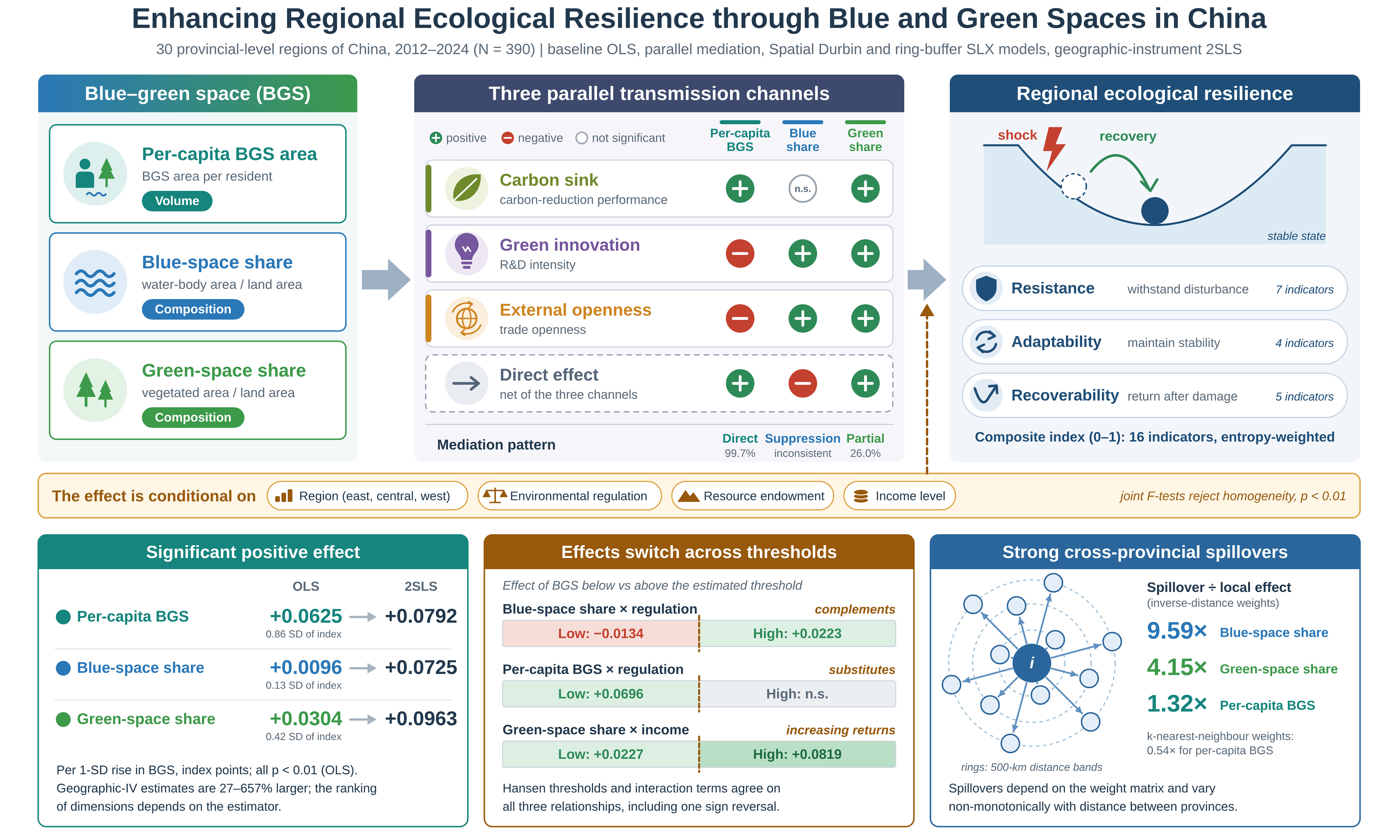
Blue-green spaces (BGSs) are key material carriers for regional ecological resilience under accelerating climate change. Using panel data for 30 Chinese provincial-level regions over 2012-2024, this study constructs a three-dimensional ecological resilience index (resistance, adaptability and recoverability) and applies spatiotemporal econometric models to examine how BGSs affect ecological resilience, through which mechanisms, and with what spatial features. (1) BGSs significantly enhance ecological resilience. With the three BGS indicators standardized to z-scores, one-standard-deviation increases in per capita BGS area, blue-space share and green-space share raise the composite resilience score (0-1 scale) by 0.0625, 0.0096 and 0.0304 index points, equivalent to 0.86, 0.13 and 0.42 standard deviations of resilience (SD = 0.0724). The effect varies across geographic, institutional, resource-based and economic dimensions and follows a nonlinear, threshold-dependent pattern. (2) BGSs work through three parallel channels: carbon sinks, green technological innovation and external openness. For blue space, the indirect effect (+0.0178) is significantly positive while the direct effect (-0.0083) is significantly negative, a suppression configuration in which the indirect-to-total ratio (186.3%) is not a conventional mediation share; green space shows partial mediation (26.0%). (3) Under the inverse-distance matrix, spillover effects exceed local effects, with indirect-to-direct ratios of 9.59, 4.15 and 1.32 for blue space, green space and per capita BGS area; this ranking is matrix-dependent (the per capita BGS ratio falls to 0.54 under the K-nearest-neighbor matrix), and spillovers vary nonmonotonically with distance. The findings inform differentiated ecological governance and coordinated cross-regional protection.
Keywords


 Download PDF
INTRODUCTION
With the acceleration of urbanization, cities worldwide are confronting a cascade of compounded risks. Under a high-emission pathway, more than two billion current urban residents are projected to experience an additional temperature increase of at least 0.5 °C by 2040, and as much as 36% of the global urban population could face mean annual temperatures of 29 °C or above; only approximately 1% would be spared any warming at all. At least 517 million urban residents - 14% of the world’s city dwellers - will be exposed to 100-year riverine flooding by 2030, and urban flood exposure has increased 3.5 times faster than rural flood exposure since 1975. At least 600 cities are projected to shift to drier climate types by 2040, exposing an additional 180 million people to water scarcity. Moreover, the ecological space that buffers these pressures is itself contracting: the average share of green area in the world’s cities fell from 19.5% in 1990 to 13.9% in 2020, over a period during which the literature came to identify networks of blue-green infrastructure as a principal instrument of equitably distributed urban climate adaptation[1]. Traditional passive restoration approaches can no longer adequately respond to the shocks generated by extreme weather and sudden environmental events. As a critical dimension of urban sustainability, ecological resilience plays a pivotal role in safeguarding ecological security, improving living environments, and advancing ecological restoration and governance[2]. The International Union for Conservation of Nature (IUCN) has issued a global standard for nature-based solutions, first published in 2020 and revised in a second edition in 2026, underscoring the need for integrative and holistic responses to such challenges and highlighting the central role of ecological resilience in climate change adaptation[3,4]. China is among the fastest-urbanizing countries in the world; its urbanization rate increased from 17.9% in 1978 to 67% in 2024[5]. This pace has resulted in a series of environmental problems, including resource depletion, air pollution, soil erosion, and biodiversity loss, and it has reshaped the regional climate[6]. The Sendai Framework for Disaster Risk Reduction 2015-2030 was the first global disaster-risk instrument to recognize ecosystem degradation as a driver of risk and ecosystem-based approaches as a means of reducing it[7]; the Political Declaration adopted at the 2023 midterm review of the Framework went further, explicitly calling on states to promote nature-based solutions and ecosystem-based approaches across all phases of disaster risk management[8]. How to draw on nature to bolster ecological resilience amid pervasive uncertainty and risk has therefore become a central research goal across ecology, urban planning, and related fields. Unlike earlier studies that focused on the quantity of single elements, research on Blue-green spaces (BGSs) integrates hydrological functions with vegetative landscapes, thereby treating the ecosystem as a whole and playing an indispensable role in enriching biodiversity and improving climate adaptive capacity[9]. Because BGSs form the material foundation for ecological resilience, optimizing their configuration is critical for enhancing the stability, disturbance resistance, and recoverability of ecosystems. Therefore, studying how BGSs enhance ecological resilience is necessary for both implementing the United Nations Sustainable Development Goals (SDGs) and for providing an urgent response to the compounded ecological risks that global climate change can cause.
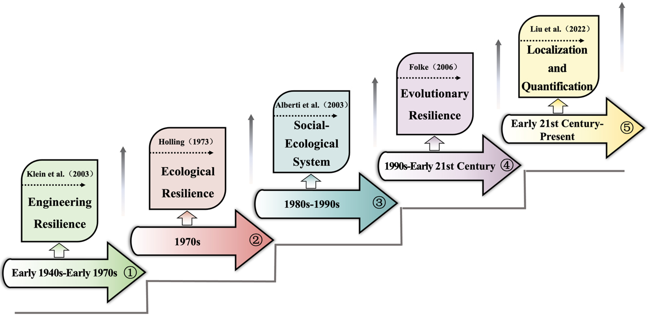
The word “resilience” comes from the Latin resilio. It originally described how quickly a system returns to equilibrium, and it covers the capacity to withstand crises, recover from them, and adapt to new conditions[10]. The concept developed in stages: engineering resilience[11], ecological resilience[10], social-ecological systems resilience[12], and evolutionary resilience[13] [Figure 1]. Through this process of conceptual evolution, it has since grown into a composite attribute that spans the social, economic, engineering, and ecological domains[14]. Ecological resilience, one of its key dimensions, was first introduced by Holling, who defined it as an ecosystem's ability to return to a stable state after a disturbance and stressed the resistance and recovery properties of natural systems[10].
Existing studies of ecological resilience have primarily examined how systemic functions are maintained and restored across spatial and temporal scales, with particular attention given to BGSs as spatial carriers that strengthen ecosystem disturbance resistance and self-regulatory capacity through natural mechanisms such as hydrological regulation and climate moderation[15,16]. The literature is also expanding from a single “BGS-carbon sink-ecological outcome” service channel internal to the ecosystem[17] to investigations of how BGSs enhance ecological resilience via economic and social factors[18] and it increasingly emphasizes the spatial differentiation and heterogeneity of ecological resilience at national or regional scales[19].
Despite these contributions, several gaps remain. First, prior research has tended to examine the influence of blue space or green space on ecological resilience in isolation[20,21], with limited attention given to BGSs from a holistic perspective. Second, in spatial terms, existing studies tend to focus on individual regions and lack systematic national-scale comparisons; the spatial spillover effects of BGSs have likewise received insufficient attention. Third, although prior work has explored the direct effect of innovation inputs on ecological performance, the indirect pathway whereby BGSs act on ecological resilience by stimulating innovation inputs has been largely overlooked, and this underlying mediation mechanism remains to be empirically substantiated.
Building on these gaps, this study utilizes panel data on 30 Chinese provincial-level administrative regions for the period 2012-2024 and applies the entropy weight method to construct a three-dimensional composite ecological resilience index encompassing resistance, adaptability, and recoverability. The first part of the analysis focuses on baseline driving effects and employs ordinary least squares (OLS) regression to identify the direct effect of BGSs on ecological resilience. The second part addresses internal mechanisms and uses a mediation model to decompose three parallel transmission channels: carbon sinks, research and development (R&D) investment, and import-export trade. The third part adopts spatial and heterogeneity perspectives, applying the spatial Durbin model and a ring-buffer spatially lagged X (SLX) model to characterize the spatial spillovers and regional differentiation of these effects. The paper concludes with policy implications for enhancing ecological resilience.
LITERATURE REVIEW AND HYPOTHESES
Influence of blue-green spaces on ecological resilience
Ecological resilience is fundamentally about maintaining and restoring systemic function, and this function in turn hinges on how the underlying material landscape is configured. As key spatial carriers of regional ecosystems, BGSs help optimize regional landscape patterns, ease environmental pressures, and reinforce both disturbance resistance and self-regulation. The earliest planning approach to incorporate BGSs is usually traced to F. L. Olmsted’s park systems, which were built in the late nineteenth century around urban water networks[22]. Blue space covers rivers, lakes, reservoirs, wetlands, and other natural or constructed water bodies, whereas green space refers to all vegetation-covered areas, such as mountainous terrain, forests, grasslands, and nature reserves[23-25]. Panarchy theory holds that ecosystems are organized as nested adaptive cycles, in which resistance, adaptability, and recoverability operate across several spatiotemporal scales and together shape the resilience profile at each hierarchical level[26]. Resistance is an urban ecosystem’s ability to withstand external disturbance[27]; it forms the foundation of ecological resilience. Adaptability is the ecosystem’s ability to maintain stability[27], and it is central to transformative development. Recoverability is the system’s ability to return to a predisturbance state after damage[27]; it underpins the restoration and enhancement of systemic function.
Consider resistance first. By acting as natural buffers inside urban ecosystems, BGSs regulate regional hydrological cycles through vegetation interception, soil infiltration, wetland retention, and channel storage. This dampens flood shocks from extreme precipitation and eases water scarcity during dry spells[15,28]. Green spaces such as grasslands and forests can also blunt the destructive forces of typhoons and geological hazards and limit anthropogenic disturbance to ecosystems[16]. The magnitude of this buffering is measurable and bounded. By fitting surface models to 53 green patches and 28 water bodies in Changsha using Landsat imagery, Qiu et al.[29] reported that the cooling effect of blue-green space increases with increasing patch size and then saturates: the cooling distance stabilizes beyond approximately 2.98 ha for blue space and 3.15 ha for green space, and the cooling magnitude saturates beyond about 4.84 ha and 4.92 ha, respectively, with the best-performing configurations delivering a cooling distance of 413.46 m for green space and a cooling magnitude of 5.17 °C for blue space. By buffering against acute shocks in this way, BGSs reduce how much an ecosystem is damaged and thus strengthen the resistance of the urban environment - although the saturation thresholds also indicate that the returns to additional areas are not unbounded, a point to which the threshold analysis in Section Hansen threshold regression returns at the provincial scale.
Adaptability comes next. On the one hand, evapotranspiration cooling, cool-island effects, and ventilation corridors allow BGSs to improve regional thermal environments, ease urban heat-island effects, and reduce the ecosystem stress associated with extreme heat and climatic variability[30]. In addition, networked BGS configurations move material and energy through corridor connectivity, agglomeration, and redundancy. This allows ecosystems to keep adjusting their structure and function under sustained urban pressure, maintain a steady state, and develop long-term adaptability[31,32].
Recoverability is the third dimension. By drawing on intact ecological structures and natural restoration processes, BGSs support biodiversity gains, better ecosystem services, and improved land quality[33]. This helps damaged ecosystems reorganize themselves and recover function after their structure or function has been impaired. The structural redundancy of BGS networks also guards against the cascading failures that disaster shocks can trigger, offering alternative pathways and buffer space for repair[34] and speeding the return of ecosystems to a healthy state.
Taken together, BGSs strengthen the resistance, adaptability, and recoverability of ecosystems and, in doing so, reinforce regional ecological resilience. We therefore propose the following:
H1. Blue-green spaces have a significant positive effect on regional ecological resilience.
Regional heterogeneity and spatial spillovers
The three sources on which this definition is drawn do not adopt identical boundaries, and the differences are borne on the measure used here. Zhang defined blue space as linear water bodies - rivers and canals - together with areal spaces such as lakes, reservoirs, wetlands, and ponds and defined green space broadly to include farmland, ecological corridors, and public open space alongside parks and protective belts at the scale of an entire municipality[23]. Xie et al. adopt a narrower green space boundary confined to vegetated land inside the developed-up district - parks, residential and roadside greenery, woodland, and nature reserves - and exclude farmland[24]. Jiao et al. share the wider conceptual boundary but operationalize it differently again: their unit of observation is a 100 m2 sampling plot scored on twelve indicators of blue-green integration rather than an area share[25]. We follow the wider, municipality-scale boundary of Zhang because the unit of analysis here is the province, and the relevant quantity is the total ecological land endowment available to the resident population, not the greenery inside a built-up perimeter. Our blue space and green space shares are accordingly area shares of total provincial territory and are therefore not directly comparable with the integration scores reported by Jiao et al.[25].
Existing studies have documented pronounced spatial differentiation in ecological resilience and in the ecological effects of blue-green space, although they do so on different objects and at different scales. Wang and Li[27] reported substantial interprovincial divergence in urban ecological resilience across China and reported that its drivers differ by region. Li et al.[35], who estimated geographically and temporally weighted regressions for prefecture-level cities in the Yangtze River Delta, reported that the contribution of blue-green space to surface cooling is unequally distributed across cities rather than uniform[27,28,30]. The underlying driving mechanisms also differ markedly across regions. In ecologically vulnerable areas, conventional economic and scientific-technological factors may even have suppressive effects on ecological resilience[31]. Furthermore, the ecological effects of BGSs themselves exhibit substantial regional dependence[35]. On the one hand, differences in natural endowments and water resource constraints across regions give rise to divergent BGS construction modes[33]; on the other hand, different types of BGSs differ in their ecosystem service provisions and thus exert uneven influences on ecosystem stability[18]. Linkages among regional systems - through population mobility and related channels - generate marked spatial associations in ecological resilience. For example, Li et al.[36] emphasized pronounced network linkages between regions in research on ecological resilience. This pattern is not confined to China’s provincial scale. Zhou et al.[37] compared ecosystem-service supply-demand relationships across four spatial scales in the Yangtze River midstream urban agglomeration and reported that their conclusion on the scale at which coupling is strongest contrasts with findings obtained for northeastern China, attributing the divergence to region-specific ecological pressure dynamics; Han et al.[38] quantified four services at six spatial scales on the Loess Plateau and reported that both the supply-demand mismatch and its dominant drivers were scale-dependent. Yang et al.[39] reported that geographical position, population distribution, economic conditions and planning policy jointly produce an uneven urban-rural development gradient that complicates relationships among ecosystem services; An et al.[40] documented systematic spatial heterogeneity in ecosystem services and their drivers at the individual, pair and bundle levels for northeastern China; and Chen et al.[41] reported that the drivers of ecosystem-service supply exhibit threshold effects rather than uniform gradients. Taken together, this evidence indicates that the ecological returns to a given natural endowment are conditioned by the regional context in which that endowment sits. Nevertheless, with respect to BGSs as an ecological element, the literature still lacks systematic national-scale empirical evidence on regional heterogeneity and spatial mechanisms.
The above considerations suggest that the impact of BGSs on ecological resilience is unlikely to be uniform; rather, it is jointly conditioned by regional developmental stage, resource endowment, and spatial structure. We therefore propose the following:
H2. The impact of blue-green spaces on ecological resilience exhibits significant regional heterogeneity.
Carbon sinks, R&D, and trade openness as mediating channels
The most direct ecological functions of BGSs are carbon sequestration and climate regulation. By absorbing CO2 and moderating microclimates, BGSs improve regional decarbonization outcomes and, in turn, reinforce ecosystem recoverability and stability - an important ecosystem service channel. As global warming intensifies, the carbon sink functions of urban green spaces have drawn increasing amounts of scholarly attention[42,43]. As nature-based solutions (NbS) have been progressively integrated into urban ecological planning[44], BGSs are being upgraded from dispersed ecological nodes to climate-adaptive infrastructure, and their carbon management functions have acquired new strategic significance[45]. Current research on the carbon sink performance of urban green spaces spans three scales: macrolevel studies of city-wide green space carbon benefits[46,47], meso-level studies of carbon performance in public green spaces[48-50], and microlevel studies of the carbon benefits of individual plant species[34,51]. Comparative accounting across ecosystem types revealed that the carbon pool was very unevenly distributed: In a study that measured subtropical forests, urban green spaces and wetlands separately within a single city, forests accounted for 72% of the total pool, whereas green spaces and wetlands accounted for 14% each[52], while urban green spaces and parks played a more important role in active carbon sequestration[45,47]. In a study of the Nanyuan waterfront green belt in Shanghai, for example, Jiang et al. reported that urban green spaces contribute positively to carbon benefits, and they reported that green space connectivity is a factor that strengthens this contribution[17]. Much of the literature treats carbon sinks as key mediating variables between BGSs and ecological outcomes, yielding the single “BGS-carbon sink-ecological outcome” pathway.
As research has advanced, scholars have recognized that the functions of BGSs extend beyond the internal ecosystem and shape regional development indirectly through their effects on economic activity and social behavior[53]. With the push for regional high-quality development, green technological innovation has gradually become a critical determinant of ecosystem stability and adaptive capacity[54].
Turning to technological innovation as a mediating channel, digital economic development can markedly increase innovation efficiency: it eases information access and management on the information side, and it allows R&D demand to be identified in good time on the market side, both of which drive green development indirectly[55]. Two recent studies establish the same conditionality at the firm level. Yi et al.[56] reported that the emission-reducing returns to green technological innovation in China’s high-end manufacturing sector depend on the environmental, social and governance (ESG) governance and digital capabilities that accompany it such that innovation alone is not sufficient; Saiyed et al.[57] reported a comparable pattern for Taiwan’s manufacturing sector, where artificial intelligence increases green innovation capacity only where absorptive capacity is already in place. Both results hold directly on the channel examined here, since they imply that the resilience returns to a green-innovation channel should be expected to vary with the institutional and technological conditions of the region rather than to be constant. Regional development quality and ecosystem conditions are also closely linked, with innovation capacity bridging the two[31]. Innovation inputs therefore accelerate technological progress and efficiency gains, and in this way, they supply the basic conditions for ecological resilience to form.
Furthermore, the relationship between ecological conditions and innovation activity has attracted increasing attention. Existing research suggests that strong ecological foundations and livable environments help attract high-caliber talent and high-end factor agglomeration, thereby supporting innovation activity[18]. As critical carriers of urban ecosystems, BGSs not only increase regional livability by improving air quality and ecological landscapes but also strengthen overall urban attractiveness and factor-agglomeration capacity. In this process, talent agglomeration and factor inflows foster knowledge exchange and technological spillover, which in turn promote R&D investment and intensify innovation activity. Accordingly, BGSs do not act directly on ecological resilience alone; rather, they indirectly influence the regulatory and risk-response capacity of regional ecosystems through innovation inputs as a mediating variable. Within this mechanism, innovation constitutes an important driving channel, prompting local governments and firms to scale up their investment in green technology R&D and to enhance ecological resilience through technological progress.
A growing body of emerging research has begun to examine the linkage between BGSs and open economic activity at the urban scale. Existing evidence suggests that high-quality ecological environments help enhance a city’s image and investment attractiveness, thereby promoting international capital inflows and the development of foreign trade[58]. Amid intensifying global urban competition, ecological livability has become an important factor influencing firms’ location decisions and cross-border investment[59]. Regions endowed with abundant BGSs often possess locational advantages along rivers, coasts, or lakeshores[31,33]; such spaces serve simultaneously as carriers of ecological resources and as nodes of external openness. Within the framework of an open economy, BGSs strengthen a city’s attractiveness within global factor flows by improving regional environmental quality and spatial amenities, thereby promoting the agglomeration of foreign direct investment[60] and the expansion of import-export trade[61].
Accordingly, we propose the following:
H3. Blue-green spaces act on regional ecological resilience through three parallel channels: (i) the enhancement of ecosystem service functions, (ii) the stimulation of green technological innovation, and (iii) the strengthening of external openness. The relative weight of these channels is expected to differ between volume-type and composition-type BGS measures.
METHODOLOGY
Indicator system
Building on the three-dimensional structure of ecological resilience, this study decomposes regional ecological resilience into resistance, adaptability, and recoverability[62-66] and constructs the corresponding evaluation indicator system. Alongside the ecological resilience indicators, BGS indicators are introduced as the core explanatory variables, capturing regional ecological-space characteristics and their influence on ecological resilience.
Dependent variable
In this paper, ecological resilience is defined as the capacity of an ecosystem to absorb disturbance, adapt to change, and rapidly recover in the face of acute shocks and chronic stress. Drawing on the existing literature[67-72], we construct a composite ecological resilience evaluation system [Table 1]. Indicators were retained according to three criteria: use in more than one of these studies, a consistent definition across all 30 provinces over 2012-2024, and no near-duplication of another indicator within the same dimension. All sixteen indicators are min-max normalized according to their direction, weighted via the entropy method, and aggregated into a composite ecological resilience score on a 0-1 scale; the composite score itself is not further standardized in the regressions.
Composite ecological resilience evaluation indicator system
| Criterion | Indicator | Direction |
| Resistance | GDP per capita (CNY/person) | − |
| Population density (persons/km2) | − | |
| Industrial wastewater discharge per unit GDP (tons per 10,000 CNY) | − | |
| SO2 emissions per km2 (tons/km2) | − | |
| Industrial soot emissions per unit GDP (tons/100 million CNY) | − | |
| Share of built-up area | − | |
| Mean PM2.5 concentration (μg/m3) | − | |
| Adaptability | Harmless treatment rate of domestic waste (%) | + |
| Urban sewage treatment rate (%) | + | |
| Volume of domestic waste removed (104 tons) | + | |
| Comprehensive utilization rate of general industrial solid waste (%) | + | |
| Recoverability | Per-capita public green-space area (m2/person) | + |
| Per-capita water resources (m3/person) | + | |
| Share of nature reserves in jurisdictional area (%) | + | |
| Forest coverage rate (%) | + | |
| Share of environmental protection in fiscal expenditure (%) | + |
Explanatory variables
The explanatory variable in this study is blue-green space, defined as the integrated material space comprising all natural and constructed open spaces and composite water bodies - a hybrid ecological space that transcends the independent states of its blue and green components. Following the existing literature[73-75], we construct the BGS indicator system along two dimensions - total scale and structure - comprising per-capita BGS area, share of blue space, and share of green space. Per-capita BGS area is measured as the ratio of total regional BGS area to end-of-year total population, reflecting per-capita BGS provision and the adequacy of aggregate supply. The share of blue space is calculated as the proportion of total natural and constructed water-body area (rivers, lakes, reservoirs, ponds, etc.) within jurisdictional land area, capturing the coverage of regional blue ecological space. The share of green space is calculated as the proportion of total vegetated area (cropland, forest, shrubland and grassland) within jurisdictional land area, capturing the coverage of regional green ecological space. All three BGS indicators are standardized to z-scores (mean 0, standard deviation 1) before they enter the regressions (Section Baseline OLS regression).
Mediating variables
Drawing on the existing literature, we select three mediating variables that correspond to the three transmission channels: carbon-reduction performance, R&D intensity, and trade openness. We measure carbon-reduction performance[76,77] as one minus the min-max normalized provincial CO2 emissions, so that higher values indicate lower emissions; it reflects regional decarbonization outcomes and ecosystem service function. We measure R&D intensity[78,79] as R&D expenditure divided by GDP, a proxy for regional green technological innovation. We measure trade openness[80] as the total value of imports and exports (104 USD), which captures the scale of external openness and factor mobility. Carbon-reduction performance enters the mediation models on its 0-1 scale, whereas R&D intensity and trade openness enter as z-scores.
Control variables
To net out confounding factors, we follow the existing literature[81] and include two control variables: economic development level (measured by per-capita disposable income) and urbanization level (measured by the share of urban population in total population), both standardized to z-scores.
Instrumental variables
For each core explanatory variable, we select a theoretically defensible instrument satisfying the exclusion restriction. For per-capita BGS area, we use topographic relief[82]: rugged terrain limits the availability of constructible and arable land and thus tends to preserve more natural BGS, while terrain - as a long-run product of geological evolution - can be regarded as approximately exogenous to short-run socioeconomic variables. For the share of blue space, we use the multi-year average precipitation over 1990-2020[83]: precipitation is the fundamental physical basis for water-body formation, and its long-run average - jointly determined by the monsoon system, topography, and latitude - is essentially a time-invariant climatic attribute. For the share of green space, we use mean slope[84]: steep terrain precludes large-scale cultivation or construction and necessitates the maintenance of vegetative cover, while slope, as a geomorphological feature, lacks a direct channel to provincial economic development.
Empirical models
Baseline OLS regression
To examine the overall effect of BGS on regional ecological resilience, the baseline specification is:
where erit is the composite ecological resilience score of province i in year t, kept on its original 0-1 scale; bgsj,it (j = 1,2,3) denote per-capita BGS area, the share of blue space and the share of green space, which enter the regression jointly; Xit is the vector of control variables (per-capita disposable income and urbanization rate); ζt denotes year fixed effects; and εit is the random error. Before estimation, the three BGS variables and the two control variables are standardized to z-scores (mean 0, standard deviation 1) over the 390 province-year observations, whereas erit is not standardized. Each αj therefore measures the change in the composite resilience score, in index points on the 0-1 scale, associated with a one-standard-deviation increase in the corresponding BGS variable, holding the other two BGS variables and the controls constant; dividing αj by the standard deviation of erit (0.0724) expresses the same effect in standard deviations of the resilience distribution. All standard deviations are computed over the 390 observations with divisor N. The model is estimated with heteroskedasticity and autocorrelation consistent (HAC; Newey-West, max-lag = 2) robust standard errors.
Multi-channel parallel mediation model
To examine the transmission mechanisms through which BGS affect ecological resilience, we follow the three-step procedure proposed[85] and construct a three-channel parallel multi-mediation system of structural equations.
Step 1: test the total effect of BGS on ecological resilience [Equation 1].
Step 2: test the effect of BGS on each mediating variable:
Step 3: test the joint effects of BGS and the mediators on ecological resilience:
where bgsit is the focal BGS variable;
Spatial econometric models
To characterize the spatial spillovers of BGS, three spatial weight matrices are constructed. The inverse-distance weight matrix (W1) uses the geodesic distance between provincial capitals, with weights equal to the inverse of distance:
where dij is the geodesic distance between provinces i and j. The K-nearest-neighbor weight matrix (W2) assigns weight 1 to each province’s four nearest neighbors and zero otherwise. The ring-buffer weight matrix (Ws) uses a 500-km step size to group neighboring provinces into five distance bands (0-500 km, 500-1,000 km, 1,000-1,500 km, 1,500-2,000 km, ≥ 2,000 km), with a separate 0/1 binary adjacency matrix constructed for each band. All matrices are row-standardized. To assess whether spatial dependence remains after conditioning on the covariates, the global Moran’s I statistic is computed on the residuals of the pooled OLS regression rather than on the resilience index itself:
where ei is the residual of observation i from the pooled OLS regression, e is the mean residual, N = 390 is the number of province-year observations, and wij are the elements of the block-diagonal matrix IT⊗W, which links provinces only within the same year (W = W1 or W2); for a row-standardized matrix S0 = N. Values above the expectation -1/(N - 1) indicate positive spatial autocorrelation, values below it indicate negative spatial autocorrelation, and values close to it indicate no spatial association.
Given that BGS and ecological resilience may both exhibit spatial spillovers, we estimate a Spatial Durbin Model (SDM):
where ρ is the spatial autoregressive coefficient and θ1 is the spatial lag coefficient for BGS. The model is estimated via maximum likelihood, with coefficients decomposed into direct, indirect, and total effects[86].
To examine distance-related heterogeneity in spatial spillovers, we further estimate a Ring-Buffer Spatially Lagged X (SLX) model:
where θs is the spatial spillover coefficient for distance band s.
Instrumental variable model
To mitigate endogeneity arising from reverse causality and omitted variables, geographic instruments are introduced in a two-stage least squares (2SLS) framework. The first-stage regression is specified as:
where bgsit is the endogenous BGS variable being instrumented; IVi denotes its time-invariant instrument (topographic relief, multi-year average precipitation, and mean slope, respectively); and
Data
The sample covers 30 provincial-level administrative units in mainland China (Tibet, Taiwan, Hong Kong, and Macau are left out because of data limitations) for 2012-2024, giving a balanced panel of 390 observations. The data come mainly from the China Statistical Yearbook, China Environment Statistical Yearbook, China Urban Construction Statistical Yearbook, together with the statistical yearbooks and environmental bulletins of the individual provinces. Blue- and green-space areas are derived from the annual 30 m China Land Cover Dataset (CLCD)[87]; the water class is classified as blue space and the cropland, forest, shrubland and grassland classes as green space, and their areas are summed by province and year to calculate the three BGS indicators.
RESULTS
Spatio-temporal evolution of regional ecological resilience in China
National-level temporal evolution
Over the sample period, the mean composite ecological resilience score climbed from 0.2897 to 0.3239, a compound annual growth rate (CAGR) of 0.93% and a cumulative gain of 11.8%. The path moved through three phases. It expanded quickly in 2012-2016, plateaued with some fluctuation in 2017-2022, and recovered again in 2023-2024, when year-on-year growth of 1.89% in 2024 marked a five-year high. Two forces drove the rebound: faster build-out of the ecological civilization institutional framework and stronger green technological innovation capacity[88,89]. The three dimensions grew at very different rates. Adaptability rose fastest at 1.92%, because it ties directly to socioeconomic systems such as industrial-structure optimization and environmental regulation[27,88]. Recoverability came next at 0.81%, since it leans mainly on the ecological baseline and natural restoration, which is slower[63]. Resistance grew slowest at 0.45%, held back by its density and land-use indicators (population density and the share of built-up area), which change slowly and in several provinces moved against resilience. The composite score is markedly right-skewed, and the recoverability dimension dominates it because its five indicators carry 64.8% of the total entropy weight [Table 1] and vary strongly across provinces. Provinces with superior ecological baselines, including Qinghai and Yunnan, sit in the long tail of the distribution, helped by high vegetation cover and biodiversity advantages [Figure 2].
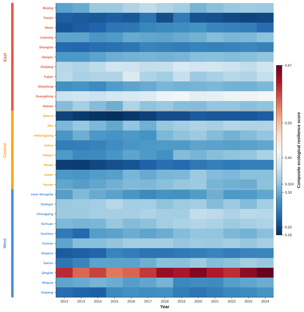
Figure 2. Spatio-temporal heat map of composite ecological resilience scores across 30 Chinese provinces (N = 390 province-year observations from 30 provinces over 2012–2024).
Regional-level temporal evolution
The gaps between provinces in 2024 are large. Qinghai ranks first at 0.6661, where recoverability dominates and supplies 75.4% of the composite score, thanks to the strong ecological baseline of high-vegetation areas such as the Three Rivers Source Area[89]. Guangdong comes second at 0.4161 and follows an “adaptability-driven” pattern: it posts the highest adaptability score in the country, a sign of its advanced economy, environmental technology, and industrial-structure optimization[90]. Zhejiang stands out as the only province whose three dimensions stay fairly balanced, which reflects strong coupling and coordination across its economic, social, and ecological system[91]. At the other end, Tianjin ranks last at 0.1997 and is the only province with negative growth, as rising population density and built-up share eroded its resistance while declines in its nature-reserve share, per-capita water resources and environmental-expenditure share eroded its recoverability; urbanization-driven contraction and fragmentation of green space of this kind has been documented for China’s large cities[92]. The growth figures show a clear late-mover catch-up effect. Gansu records the highest CAGR at 2.44%, driven by both recoverability (its nature-reserve share rose from 10.8% to 16.0% and per-capita public green space from 9.5 to 15.4 m2) and resistance (sharp falls in SO2 and industrial-soot intensity), consistent with evidence that sustained ecological restoration strengthens key regulating services[93]. Central and western provinces generally grow faster than the high-baseline eastern coastal provinces, which points to a technological-diffusion dividend and to the catch-up advantage that latecomer regions enjoy from a low base[94] [Table 2].
Top-5 and bottom-5 provinces by CAGR
| Rank | Fastest-growing | CAGR | Rank | Slowest-growing | CAGR |
| 1 | Gansu | 2.44% | 26 | Ningxia Hui Autonomous Region | 0.22% |
| 2 | Henan | 2.38% | 27 | Hainan | 0.21% |
| 3 | Guizhou | 2.11% | 28 | Guangxi Zhuang Autonomous Region | 0.21% |
| 4 | Jiangxi | 1.62% | 29 | Fujian | 0.19% |
| 5 | Shaanxi | 1.57% | 30 | Tianjin | −0.87% |
Regional convergence of ecological resilience
The three macro-regions display markedly different resilience structures. The western region attains the highest composite score but exhibits a clear adaptability shortfall, owing to its strong recoverability - rooted in high vegetative cover - being undermined by lagging industrial restructuring[36,95]. The eastern region leads in adaptability but trails in recoverability, reflecting its environmental-technology advantages alongside the squeezing of its ecological baseline by urbanization[36,95]. The eastern region is the most balanced across the three dimensions, with a dimensional coefficient of variation of 0.049 against 0.291 for the central region, while the central region records the lowest composite score, indicating moderate but uneven coupling among its economic, social, and ecological subsystems[36,94]. Temporally, the central region grows fastest (CAGR 1.258%) and the eastern region slowest (CAGR 0.655%), with the western region intermediate (CAGR 0.991%). Here, macro-regional scores are calculated as unweighted means of the underlying provincial scores across the 11 eastern, 8 central, and 11 western provinces; the regional balance coefficient is defined as the population standard deviation of a region’s three mean dimension scores (resistance, adaptability, and recoverability) in 2024 divided by their mean; and the regional CAGR is computed as [(mean regional score in 2024 / mean regional score in 2012)1/12 − 1] × 100%, whereas Figure 3 reports nationwide inter-provincial dispersion. Inter-provincial convergence follows a U-shaped trajectory in the dispersion measures: slow convergence during 2012-2021 gives way to mild divergence during 2022-2024, with the turning point in 2021 (Gini trough = 0.1018) and the range ratio rising to 3.34 in 2024, indicating that extreme disparities have not fundamentally narrowed. The early convergence is driven by the rapid catch-up of low-base western provinces[36,96], whereas the subsequent divergence reflects the increasing differentiation between resource-based and governance-driven resilience pathways across provinces[36,96] [Figure 3].
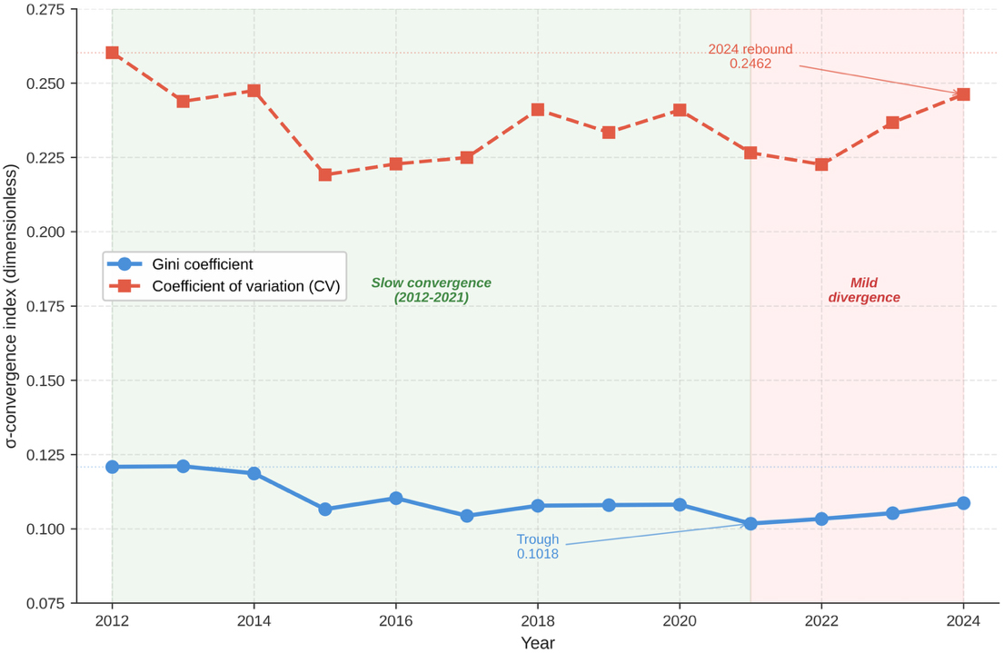
Figure 3. σ-convergence analysis. Each annual dispersion measure is calculated across 30 provinces over 13 years (N = 390 province-year observations, 2012–2024).
National-level spatial evolution
To provide a more intuitive characterization of the spatial pattern and dynamic evolution of provincial ecological resilience, we map the classified composite indices for four reference years (2012, 2016, 2020, and 2024; Figure 4). Provincial ecological resilience in China displays a persistent baseline pattern of “higher in the west and lower in the east; higher in the south and lower in the north”, accompanied by a structural shift characterized by “the rise of the east and the entrenchment of the north”. By 2024, a tripartite configuration has emerged, with a polar core in the northwest, hotspots in eastern China, and cold spots in northern China, confirming the dual logic of “natural-baseline dominance and innovation-driven differentiation” in the evolution of provincial ecological resilience. The west-high pattern should be read with one qualification: Qinghai records the highest composite score in every reference year, so the western average is shaped disproportionately by a single province[36].
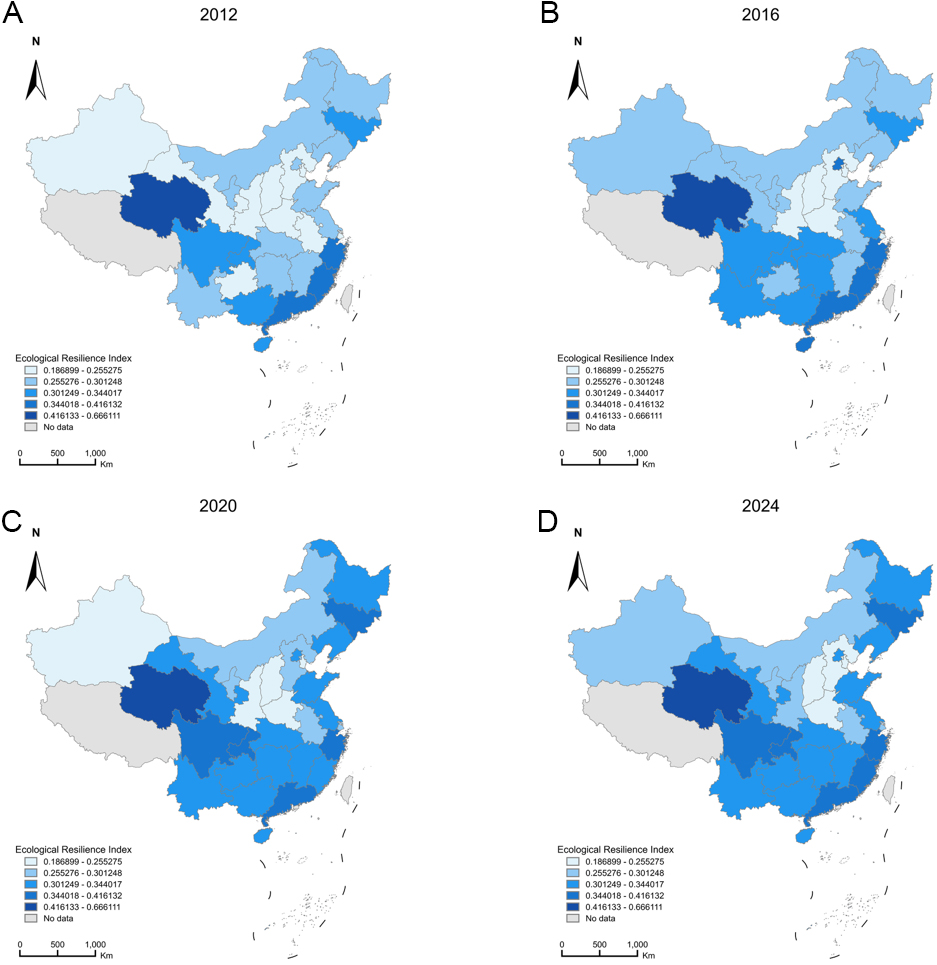
Figure 4. Spatial evolution of the composite provincial ecological resilience index in China, 2012–2024. Provinces for which the index could not be computed (Tibet, Taiwan, Hong Kong and Macao) are shown in grey. Each mapped year includes n = 30 provinces with available scores (N = 390 province-year observations over 2012–2024). Administrative boundaries, including the national boundary and the dashed-line boundary in the South China Sea, follow the standard map of China issued by the Ministry of Natural Resources of China under approval number GS(2023)2765, obtained from the Standard Map Service at http://bzdt.ch.mnr.gov.cn/ (accessed 6 September 2026); the boundaries were not modified. Map lines do not necessarily depict accepted national boundaries.
Effect of blue-green spaces on ecological resilience
Baseline regression
The baseline regression results show that all three core explanatory variables - per-capita BGS area, share of blue space, and share of green space - are significantly positive at the 1% level [Table 3]. Because the three BGS variables are standardized to z-scores while the resilience score is kept on its 0-1 scale (Section Baseline OLS regression), each coefficient is the change in the composite score, in index points, associated with a one-standard-deviation increase in the corresponding BGS variable. A one-standard-deviation increase in per-capita BGS area raises the composite resilience score by 0.0625 index points, corresponding to 0.86 standard deviations of the resilience distribution (Table 4, “z-score of resilience” row): the aggregate dimension exerts the largest and most robust effect, providing the foundational support for regional ecological resilience and corroborating the cumulative impact of large-scale restoration programs such as the Grain-for-Green and Natural Forest Protection initiatives. A one-standard-deviation increase in the share of green space raises ecological resilience by 0.0304 index points (0.42 standard deviations); this intermediate-magnitude effect underscores the multifunctional role of forests and grasslands - air purification and climate regulation among others - as critical structural drivers of resilience, whose synergistic regulating services in water conservation and carbon storage have been amply documented[91,93]. A one-standard-deviation increase in the share of blue space raises ecological resilience by 0.0096 index points (0.13 standard deviations), indicating that water bodies and wetlands also contribute significantly, albeit with smaller marginal effects, through more complex mechanisms; sponge-city pilots have already enhanced urban aquatic resilience. Among the controls, per-capita disposable income is significantly positive, reflecting the supportive role of economic development in ecological investment; the urbanization coefficient is marginally significant at the 10% level and negatively signed, suggesting that excessive urbanization may weaken the natural recovery capacity of ecosystems.
Baseline regression results
| Variable | Coefficient | Std. Error | t | P |
| bg_percap | +0.0625*** | 0.0051 | 12.34 | 0.0000 |
| blue_share | +0.0096*** | 0.0037 | 2.60 | 0.0093 |
| green_share | +0.0304*** | 0.0035 | 8.63 | 0.0000 |
| income | +0.0306*** | 0.0078 | 3.94 | 0.0001 |
| urban | -0.0123* | 0.0071 | -1.75 | 0.0807 |
| Year FE | Yes | |||
| N | 390 | |||
| R 2 | 0.6115 | |||
These results validate H1: BGS exert a significant positive effect on regional ecological resilience along both the aggregate and structural dimensions.
Summary of baseline robustness checks
| Test category | Specification | bg_percap | blue_share | green_share | N |
| Standard errors | Province-clustered SE | 0.0625*** (0.0102) | 0.0096 (0.0072) | 0.0304*** (0.0072) | 390 |
| HC3 robust SE | 0.0625*** (0.0035) | 0.0096*** (0.0024) | 0.0304*** (0.0023) | 390 | |
| Driscoll-Kraay SE | 0.0625*** (0.0018) | 0.0096*** (0.0012) | 0.0304*** (0.0010) | 390 | |
| Fixed effects | Two-way FE (year + province) | -0.0137 (0.0463) | -0.0083 (0.0100) | -0.0845* (0.0452) | 390 |
| Outliers/sub-samples | 1%/99% winsorization | 0.0616*** (0.0048) | 0.0092** (0.0036) | 0.0303*** (0.0035) | 390 |
| 5%/95% winsorization | 0.0407*** (0.0115) | 0.0049 (0.0044) | 0.0304*** (0.0065) | 390 | |
| Excluding four municipalities | 0.0625*** (0.0050) | 0.0149*** (0.0051) | 0.0239*** (0.0031) | 338 | |
| Excluding COVID years (2020-2022) | 0.0620*** (0.0055) | 0.0087** (0.0040) | 0.0301*** (0.0040) | 300 | |
| Omitted variables / reverse causality | Additional controls | 0.0710*** (0.0047) | -0.0017 (0.0036) | 0.0282*** (0.0028) | 390 |
| Lagged core regressors (one period) | 0.0620*** (0.0054) | 0.0093** (0.0039) | 0.0301*** (0.0036) | 360 | |
| Outcome measurement | Quantile rank of resilience | 0.1296*** (0.0134) | 0.0002 (0.0189) | 0.1442*** (0.0199) | 390 |
| z-score of resilience | 0.8628*** (0.0699) | 0.1321*** (0.0508) | 0.4192*** (0.0486) | 390 | |
| Placebo (Fisher randomization) | Fisher P = 0.0000 | Fisher P = 0.0180 | Fisher P = 0.0000 | — | |
Robustness checks
To check that the baseline results hold up, we estimate twelve alternative specifications and run a Fisher randomization placebo test (Table 4; thirteen checks in total). The coefficients on per-capita BGS area and the green-space share are positive and significant in every specification except the two-way fixed-effects model; the blue-space coefficient is positive in ten of the twelve specifications - the exceptions being the two-way fixed-effects model (-0.0083) and the specification with additional controls (-0.0017) - and is close to zero under the quantile-rank transformation (+0.0002), which is consistent with its effect operating mainly through the mediating channels examined in Section Parallel multi-channel mediation analysis. After we add further controls, the blue-space coefficient turns statistically insignificant, which fits the idea that the mediating channels absorb its effect (see Section Parallel multi-channel mediation analysis). When we measure the dependent variable differently, the blue-space coefficient falls to zero under the quantile-rank transformation, a sign that it is sensitive to how the outcome is measured and that its causal channel is mainly indirect. The two-way fixed-effects specification is the one exception. Adding province fixed effects reverses the sign of all three coefficients, with the green-space share becoming significantly negative at the 10% level (-0.0845). This follows from the identifying variation available rather than from evidence against the relationship: BGS measures are structural variables with almost no within-province movement over the sample period, the within-province component accounting for 0.07% of total variance for per-capita BGS area, 1.42% for the blue-space share, and 0.09% for the green-space share. Province fixed effects absorb essentially all of the cross-provincial variation on which identification rests. We therefore retain year fixed effects as the baseline and report the two-way results alongside them. In the placebo test, the actual coefficients of all three variables fall well outside the 95% confidence intervals of the placebo distributions, with Fisher P-values of 0.0000, 0.0180, and 0.0000, which confirms that the estimated relationships are genuine rather than chance. Multicollinearity diagnostics return variance inflation factors (VIFs) below 5 for every variable - 1.26 for per-capita BGS area, 1.54 for the share of blue space, and 1.37 for the share of green space - all far under the usual threshold of 10. The baseline results are thus highly robust, and the positive effect of BGS on regional ecological resilience holds across several dimensions [Figure 5].
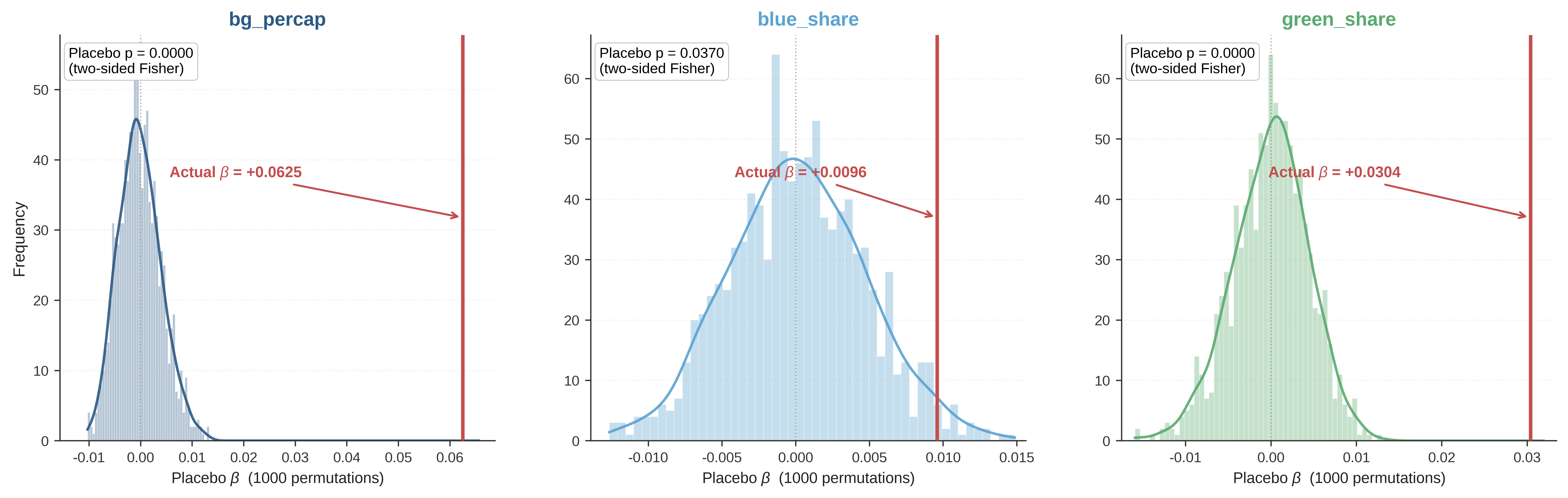
Figure 5. Placebo tests for the core explanatory variables (1,000 random permutations). Each permutation is estimated on the balanced panel of N = 390 province-year observations from 30 provinces over 2012–2024; vertical dashed lines indicate the actual baseline OLS point estimates. OLS: Ordinary least squares.
Because the entropy method assigns weights endogenously from the dispersion of the indicators themselves, the resulting index, and any inference drawn from it, could in principle be an artifact of that particular weighting rule. We therefore recomputed the composite index under the four alternatives and re-estimated the baseline specification under each [Table 5].
Composite resilience index under alternative weighting and aggregation schemes
| Scheme | Pearson r | Spearman ρ | Kendall τ | bg_percap | blue_share | green_share |
| Entropy weighted-sum (published) | 1.0000 | 1.0000 | 1.0000 | +0.8628*** | +0.1321*** | +0.4192*** |
| Entropy weighted-sum (recomputed) | 1.0000 | 1.0000 | 0.9996 | +0.8631*** | +0.1321*** | +0.4189*** |
| Equal-weight weighted-sum | 0.5801 | 0.7725 | 0.5793 | +0.2259*** | +0.1057* | +0.4941*** |
| Entropy-TOPSIS | 0.8528 | 0.6405 | 0.4884 | +0.8800*** | +0.1182*** | +0.0592 |
| Equal-weight TOPSIS | 0.7674 | 0.7337 | 0.5407 | +0.5456*** | +0.2214*** | +0.3069*** |
Two results should be separated. First, the entropy procedure is reproducible to within rounding error: recomputing the weights from the sixteen raw indicators and reaggregating returns weights that differ from the published ones by at most 0.00016 and an index whose mean absolute deviation from the published series is 0.00016 (Pearson r = 0.9999998, displayed as 1.0000 in Table 5; Kendall τ = 0.9996), with BGS coefficients that differ only in the fourth decimal place; the estimates are not sensitive to undocumented implementation choices. Second, the sensitivity of the findings depends on which aspect of the aggregation is varied. Within the weighted-sum family, replacing entropy weights with equal weights preserves the positive signs of all three BGS coefficients; all remain significant at the 10% level, although the blue-space coefficient is no longer significant at the 1% level, even though the two indices themselves correlate at only r = 0.58; the estimated effects are considerably more stable than the index. Across aggregation families, the picture is more mixed: under entropy-TOPSIS (technique for order preference by similarity to an ideal solution), the per capita BGS area (+0.8800) and the blue-space share (+0.1182) remain positive and significant, whereas the green-space share becomes insignificant (+0.0592).
The divergence across aggregation families reflects a conceptual difference rather than an estimation artefact. Weighted-sum aggregation is compensatory in that a deficit on one dimension can be offset by a surplus on another, whereas TOPSIS ranks units by their distance to an ideal point and is therefore substantially noncompensatory. The resilience concept developed in Section LITERATURE REVIEW AND HYPOTHESES, in which resistance, adaptability and recoverability are mutually substitutable contributors to a system’s capacity to absorb and recover from shocks, is compensatory by construction, and the weighted-sum index is retained on that ground. Under a noncompensatory conception, the green space effect is the least firmly established of the three.
Heterogeneity and threshold effects
Multi-dimensional heterogeneity
Substantial inter-provincial heterogeneity in China implies that the marginal effects of BGS may be non-uniform. We test for heterogeneity along four dimensions: macro-economic region, environmental-regulation intensity, resource endowment, and economic development level. Joint F-tests reject homogeneity at the 1% level in all cases [Table 6], confirming H2.
Multi-dimensional heterogeneity tests
| Variable | Three economic belts | Environmental regulation intensity | Resource endowment | Economic development level | |||||
| Eastern (N = 143) | Central (N = 104) | Western (N = 143) | High regulation (N = 195) | Low regulation (N = 195) | Resource-based (N = 143) | Non-resource-based (N = 247) | High income (N = 195) | Low income (N = 195) | |
| bg_percap | -0.5792*** (0.0795) | +0.1216*** (0.0354) | +0.0324*** (0.0102) | +0.0308*** (0.0066) | +0.0678*** (0.0062) | +0.0442*** (0.0085) | -0.0725** (0.0339) | +0.0128* (0.0067) | +0.0697*** (0.0044) |
| blue_share | +0.0181*** (0.0066) | +0.0429*** (0.0153) | +0.2528*** (0.0414) | +0.0210*** (0.0054) | -0.0052 (0.0064) | +0.1900*** (0.0218) | +0.0158*** (0.0029) | +0.0075 (0.0080) | +0.0344*** (0.0069) |
| green_share | +0.1205*** (0.0218) | +0.0473 (0.0299) | +0.0149*** (0.0050) | +0.0814*** (0.0103) | +0.0245*** (0.0091) | +0.0123*** (0.0035) | +0.0949*** (0.0100) | +0.0674*** (0.0107) | +0.0250*** (0.0046) |
| Year fixed effects | Yes | Yes | Yes | Yes | Yes | Yes | Yes | Yes | Yes |
| Joint F test | F = 51.89, P = 0.0000*** | F = 41.53, P = 0.0000*** | F = 26.78, P = 0.0000*** | F = 78.85, P = 0.0000*** | |||||
For the three macro regions, per-capita BGS area has a negative and statistically significant coefficient in the east (−0.5792***; SE = 0.0795; P < 0.01). The unconditional correlation between per-capita BGS area and ecological resilience in this subsample is positive (+0.28), whereas the estimated coefficient becomes negative after conditioning on income and urbanization. Per-capita BGS area is more closely correlated with these controls in the eastern subsample than nationally (variance inflation factor 4.13 versus 1.26 nationally), leaving less independent residual variation from which to estimate its conditional association. The statistically significant negative coefficient should therefore be interpreted as a conditional partial association within this specification, rather than as evidence that reducing BGS area would improve ecological resilience. The positive and significant coefficients on the blue- and green-space shares (+0.0181*** and +0.1205***) indicate that structural optimization of BGS composition is the primary operative margin in the east. This pattern is consistent with the transition from incremental volumetric expansion to stock and quality optimization observed in densely urbanized regions such as the Yangtze River Delta and the Pearl River Delta. In the central region, per-capita BGS and the blue-space share are simultaneously significant and positive, placing the region at an intermediate stage in which both quantity and structure remain salient and at which marginal returns to expansion are highest; the central region’s transitional position between east and west affords scope for both volume supplementation and structural upgrading. In the west, the blue-space share has the largest coefficient (0.2528), reflecting the high marginal value of blue space in water-scarce environments, where the relative expansion of blue space exerts the strongest leverage on ecological resilience; the elasticity of ecological services such as cooling, humidification, and biodiversity provision in arid-region wetlands and oases substantially exceeds that of comparable ecosystems in humid regions.
For environmental-regulation intensity, the sample is divided into high- and low-regulation provinces. Following Zhang and Ren[67], regulation intensity is measured by an entropy-weighted index of the operating costs of industrial wastewater and waste-gas treatment facilities, and provinces are divided at the median of their 2012-2024 mean index (see the note to Table 6). The high-regulation group amplifies the marginal effects of the two structural variables - green-space share and blue-space share - corroborating the “institutional complementarity” hypothesis: regulatory stringency forms a positive feedback loop with ecological space, and strict environmental regulation is a prerequisite for the realization of ecological value embedded in blue and green spaces. Policy instruments such as environmental inspections and ecological-redline delineation translate ecological protection from paper to ground in high-regulation jurisdictions. By contrast, per-capita BGS area exerts a larger effect in low-regulation provinces, where volumetric supplementation translates more directly into ecological output.
For resource endowment, the sample is divided into resource-based and non-resource-based provinces. With reference to the State Council’s National Sustainable Development Plan for Resource-Based Cities (2013-2020), the 11 provinces in which resource extraction and processing industries hold a prominent position are classified as resource-based (see the note to Table 6). Resource-based provinces are more reliant on per-capita BGS volume and the blue-space share, reflecting the dependence of their resilience-building on natural-resource stocks. Non-resource-based provinces are more responsive to the green-space share, suggesting that, absent resource advantages, the active cultivation of green ecological space becomes a key resilience-enhancement pathway.
For economic development level, the sample is divided into high- and low-income groups according to the median of per-capita disposable income by year. Per-capita BGS area and the blue-space share exert larger effects in the low-income group, reflecting the diminishing marginal returns to absolute provision. The green-space share, by contrast, exerts a larger effect in the high-income group, consistent with the Environmental Kuznets Curve (EKC)[97], which posits that demand for environmental quality rises with income.
Hansen threshold regression
To identify the boundaries of heterogeneity more precisely, we employ Hansen’s panel threshold regression[98], with per-capita disposable income and environmental-regulation intensity as threshold variables [Figure 6].
Figure 6. Hansen single-threshold regression results (income and environmental regulation). LR: Likelihood-ratio-type improvement statistic LR(γ) = N[RSSlinear − RSSthreshold(γ)] / RSSthreshold(γ), which attains its maximum at the estimated threshold
Figure 6 plots the likelihood-ratio-type improvement statistic LR(γ) = N[RSSlinear − RSSthreshold(γ)] / RSSthreshold(γ) across the candidate threshold values for each pairing, where RSSlinear and RSSthreshold(γ) denote the residual sums of squares of the linear single-regime model and the two-regime threshold model evaluated at candidate threshold γ, respectively. The estimated threshold
When per-capita disposable income is the threshold variable, all three core variables reject the single-slope hypothesis at the 1% level, indicating a significantly non-linear relationship between BGS and ecological resilience. Per-capita BGS area and the blue-space share exhibit diminishing marginal returns: once the income threshold is crossed, the returns to incremental BGS volume or to expanding the blue-space share decline markedly. The green-space share, by contrast, exhibits increasing marginal returns: after the threshold, its coefficient rises from +0.0227 to +0.0819, further supporting the EKC proposition that demand for environmental quality intensifies with rising income. When environmental-regulation intensity is the threshold variable, all three variables again exhibit significant thresholds. Per-capita BGS area has a larger effect in the low-regulation regime and becomes insignificant in the high-regulation regime, indicating that, in institutionally weaker jurisdictions, extensive volumetric supplementation remains the dominant resilience-building strategy. The blue-space share is significantly negative in the low-regulation regime but significantly positive in the high-regulation regime, indicating that strict environmental regulation is a prerequisite for blue space to produce positive effects: in the absence of regulation, waterfront development may induce encroachment and pollution that erode rather than enhance resilience. The green-space share is significantly positive only in the high-regulation regime, again consistent with an amplifying role of institutional intensity on the ecological value of green space, although this specification shows the smallest improvement statistic among the six (LR = 12.44 against 25.3-85.3 for the other pairings) and places only 39 of the 390 observations in the low-regulation regime, so the green-space result under this threshold variable should be read as indicative.
The income threshold for per-capita BGS area (0.133 in z-score units) corresponds to a per-capita disposable income of about CNY 30,500. Beijing and Shanghai lie above it throughout 2012-2024, whereas Yunnan, Guizhou, Gansu and Qinghai remain below it; the other 24 provinces cross it upward as nominal income rises, beginning with the eastern coastal provinces (Zhejiang in 2014, Tianjin in 2015, Jiangsu in 2016, Guangdong in 2017 and Fujian in 2018) and followed by the remaining provinces between 2019 and 2024. The higher income thresholds for the green- and blue-space shares are crossed in a similar order at later dates. For environmental regulation (threshold 0.193), Jiangsu, Shandong, Zhejiang, Hebei, Guangdong and Shanxi lie above the threshold throughout, whereas Beijing, Tianjin, Chongqing, Hainan, Jilin, Heilongjiang, Ningxia, Gansu, Qinghai, Guizhou and Yunnan lie below it; Henan, Anhui, Inner Mongolia, Sichuan, Hubei, Jiangxi, Shaanxi and Xinjiang cross it upward between 2013 and 2024 as their treatment expenditure increases, while Shanghai falls below it after 2012.
Multi-dimensional non-linear interaction effects
The threshold models in Section Hansen threshold regression partition the sample at estimated cut-points and are therefore restricted to a discrete characterization of non-linearity, in which the BGS effect takes one of two values on either side of a single threshold. To allow the effect to vary continuously with the conditioning variable, and to allow it to do so jointly across the three BGS dimensions, we augment the baseline specification with multiplicative interaction terms [Table 7]. The interaction specifications raise the explained variance from 0.6115 in the baseline to 0.7281 and 0.6779, respectively, indicating that the conditioning is quantitatively consequential rather than incidental.
Interaction effects between BGS and environmental regulation / income
| Variable | (1) BGS × Environmental regulation | (2) BGS × Income |
| bg_percap | +0.0152*** (0.0056) | +0.0592*** (0.0109) |
| blue_share | -0.0069* (0.0036) | +0.0160*** (0.0039) |
| green_share | +0.0289*** (0.0045) | +0.0356*** (0.0049) |
| Moderator | -0.0160*** (0.0045) | +0.0458*** (0.0104) |
| bg_percap × Moderator | -0.0508*** (0.0053) | -0.0061 (0.0117) |
| blue_share × Moderator | +0.0082*** (0.0023) | -0.0027 (0.0037) |
| green_share × Moderator | +0.0116 (0.0074) | +0.0195*** (0.0048) |
| Year fixed effects | Yes | Yes |
| N | 390 | 390 |
| R 2 | 0.7281 | 0.6779 |
Three coefficients carry the substantive content. The interaction between per-capita BGS area and environmental regulation is negative and significant (-0.0508), so that the marginal contribution of BGS volume declines as regulatory intensity rises: regulation and natural endowment are substitutes in producing ecological resilience, and provinces with weaker regulatory capacity depend more heavily on the BGS stock they happen to possess. The interaction between the blue-space share and environmental regulation runs in the opposite direction (+0.0082): water bodies and regulation are complements. This asymmetry is not arbitrary. The ecological services of water surfaces, such as retention capacity, water quality and aquatic habitat, are realized only when supported by treatment infrastructure and enforced management regimes; absent these, additional water surface area does not translate into resilience. Finally, the interaction between the green-space share and income is positive and significant (+0.0195), consistent with returns to green space rising with the maintenance expenditure, planting quality and accessibility that higher-income provinces can sustain. These estimates should be read alongside the threshold results, which they corroborate under a different functional-form restriction (Section Convergent evidence from two nonlinear specifications).
Taken together, the analyses establish four-fold heterogeneity - geographic, institutional, resource-based, and economic - in the effect of BGS on ecological resilience, and the threshold regression confirms a clear non-linear boundary, providing direct evidence for the design of region-specific ecological policy.
Parallel multi-channel mediation analysis
The transmission mechanisms by which BGS influence ecological resilience are further interrogated via a parallel multi-channel mediation analysis. We construct a three-channel parallel structural equation model and test whether BGS positively promote ecological resilience through three channels: improved decarbonization outcomes, the stimulation of green technological innovation, and the strengthening of external openness [Table 8 and Figure 7].
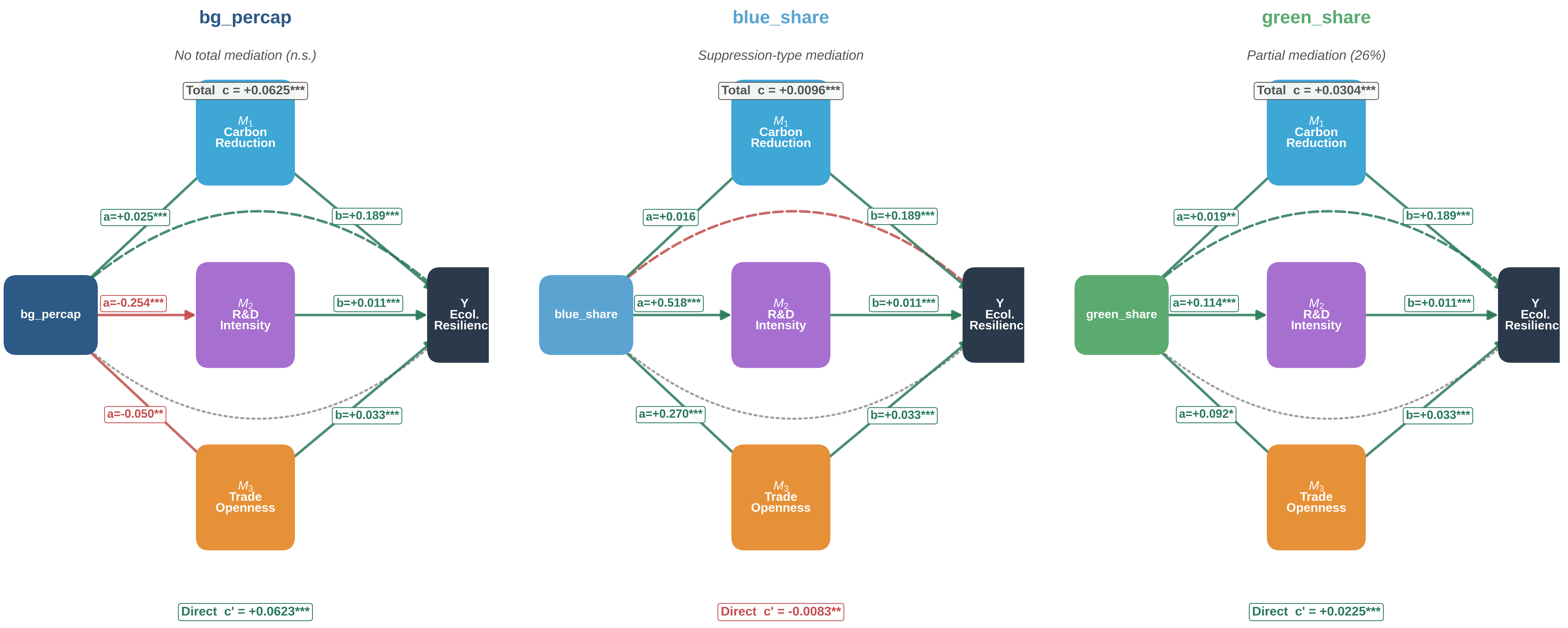
Figure 7. Decomposition of the three-channel parallel mediation effects. Estimates are based on N = 390 province-year observations from 30 provinces over 2012-2024, with indirect-effect significance tested using B = 1,000 bootstrap resamples. ***P < 0.01, **P < 0.05, *P < 0.10; n.s.: Not statistically significant.
Decomposition of the three-channel parallel mediation effects
| Mediating Channel | bg_percap | blue_share | green_share |
| a (X → M) b (M → Y) Indirect Effect | a (X → M) b (M → Y) Indirect Effect | a (X → M) b (M → Y) Indirect Effect | |
| Carbon reduction effect | +0.0250*** (0.0096) +0.1891*** (0.0274) +0.0047** | +0.0162 (0.0140) +0.1891*** (0.0274) +0.0031 | +0.0189** (0.0088) +0.1891*** (0.0274) +0.0036** |
| R&D intensity | -0.2544*** (0.0333) +0.0113*** (0.0043) -0.0029** | +0.5180*** (0.0443) +0.0113*** (0.0043) +0.0059*** | +0.1138*** (0.0431) +0.0113*** (0.0043) +0.0013* |
| Trade openness | -0.0497** (0.0204) +0.0329*** (0.0032) -0.0016** | +0.2699*** (0.0231) +0.0329*** (0.0032) +0.0089*** | +0.0919* (0.0486) +0.0329*** (0.0032) +0.0030* |
| Total effect c | +0.0625*** | +0.0096*** | +0.0304*** |
| Direct effect c' | +0.0623*** | -0.0083** | +0.0225*** |
| Total indirect effect Σa·b | +0.0002 (n.s.) | +0.0178*** | +0.0079*** |
| Mediating effect proportion | 0.3% | 186.3% | 26.0% |
The three indirect channels operate in different directions for per-capita BGS area: a positive contribution via decarbonization (+0.0047) is offset by negative contributions via R&D intensity (-0.0029) and trade openness (-0.0016), so that the three channels largely cancel and the total indirect effect (+0.0002) is statistically indistinguishable from zero [bootstrap 95% confidence interval (CI) contains zero]; the direct effect (+0.0623) accounts for 99.7% of the total effect. This indicates that per-capita BGS area operates primarily through a direct channel: BGS volume itself is the core embodiment of natural capital and directly underpins ecological resilience, corroborating the direct supply effect of large-scale national greening programs such as Grain-for-Green and Natural Forest Protection. Expansion of BGS volume is, in itself, a highly effective resilience-enhancement pathway. For the blue-space share, all three indirect channels are positive in sign, but only the R&D-intensity (+0.0059) and trade-openness (+0.0089) channels are statistically significant; the carbon-reduction channel (+0.0031) is not, because the corresponding a-path (+0.0162, SE 0.0140) is insignificant. The direct effect is significantly negative (-0.0083) while the indirect effect is significantly positive (+0.0178), so that the indirect effect exceeds the total effect and their ratio reaches 186.3% (computed from unrounded estimates; see the note to Table 8). Because the direct effect is significantly negative while the indirect effect is significantly positive, this is a suppression (inconsistent-mediation) configuration rather than full mediation, and the 186.3% ratio should not be interpreted as a share of a mediated total effect. Substantively, the blue-space share raises ecological resilience only through derivative economic and social mechanisms, while its direct partial association, holding those mechanisms fixed, is negative, plausibly because water-surface share substitutes for vegetated land at a given territorial area. Among these, the trade-openness channel contributes the most (+0.0089), highlighting the role of river-, coast-, and lake-adjacent location advantages as a key mechanism through which blue space strengthens resilience. The R&D innovation channel contributes next (+0.0059), reflecting the supportive role of water-related green-technology innovation in restoring aquatic ecosystems; the ecosystem-service channel via decarbonization contributes the least (+0.0031). For the green-space share, both the direct effect (+0.0225) and the total indirect effect (+0.0079) are significantly positive, with the direct channel contributing approximately 74% and indirect channels approximately 26%, consistent with a partial-mediation pattern. All three indirect channels are positive and significant, indicating that green-space structure directly provides ecosystem functions while also operating indirectly through R&D, openness, and carbon-sink channels - a configuration consistent with the experience of China’s Forest City program, in which urban green spaces directly improve environmental conditions through air purification and climate regulation while concurrently catalyzing green-technology R&D and low-carbon industries such as eco-tourism.
To assess the robustness of the three-channel model, we add an industrial-upgrading index as a fourth mediating channel [Table 9].
Mediation results with an industrial-structure channel
| Variable | Carbon | R&D | Openness | Industry (-) | Direct c′ |
| bg_percap | +0.0044** | -0.0045** | -0.0015** | -0.0008 | +0.0650*** |
| blue_share | +0.0029 | +0.0092*** | +0.0083*** | -0.0020 | -0.0088*** |
| green_share | +0.0033** | +0.0020** | +0.0028* | -0.0009 | +0.0230*** |
With the industrial-structure channel included, the signs and significance of the original three channels remain essentially unchanged; the industrial-structure channel produces small negative mediation effects across all three variables, but its magnitude is far smaller than that of the three original channels and does not affect the main conclusions. The mediation analysis thus supports H3 in its revised, dimension-contingent form: the channel structure is not uniformly positive, and it is precisely this heterogeneity across BGS dimensions that carries the substantive message. It reveals markedly distinct mediation profiles for the three core variables, illustrating the heterogeneous mechanisms operating across the dimensions of BGS.
Spatial spillover effects
The preceding analyses assume independence across provinces in the standard panel framework, but ecosystems are spatially continuous: a province’s BGS may influence ecological resilience not only locally but also in neighboring provinces. We use the SDM and the ring-buffer SLX model to identify these spatial spillovers systematically.
We first test for spatial dependence in the residuals of the pooled OLS regression using the global Moran’s I [Table 10].
OLS residual spatial autocorrelation tests
| Weight matrix | Moran’s I | LM-Lag | LM-Error | Robust LM-Lag | Robust LM-Error | LM-SARMA |
| W1 inverse distance | +0.034** | 14.90*** | 4.21** | 23.46*** | 12.76*** | 27.67*** |
| W2 K = 4 NN | +0.167*** | 46.57*** | 25.07*** | 22.30*** | 0.80 | 47.36*** |
Over 2012-2024, OLS residuals exhibit significantly positive Moran’s I values under both weight matrices (+0.034 under inverse-distance and +0.167 under K = 4 nearest-neighbor), strongly rejecting independence across provinces. The LM-test family indicates the coexistence of spatial lag and spatial error dependence, and the Robust LM tests identify spatial lag as the dominant structure; the SDM is therefore appropriate.
The SDM effect decompositions [Tables 11 and 12] show that, under W1, the indirect (cross-provincial) effects of all three core variables significantly exceed their local direct effects: the indirect-to-direct ratios are 1.32, 9.59, and 4.15 for per-capita BGS, blue-space share, and green-space share, respectively. BGS are thus typical regional public goods, with their contribution to ecological resilience realized primarily through cross-provincial spillovers - an outcome consistent with the inherently trans-administrative nature of atmospheric circulation, river networks, and species migration. Upwind shelterbelts attenuate downwind dust intrusion, and upstream water conservation directly benefits downstream water supply and aquatic ecology. Under W2, the direct effect of the blue-space share (-0.0002) is statistically insignificant while its indirect effect (+0.0335) remains significantly positive, yielding an asymmetric “direct = 0, indirect > 0” pattern. This indicates that, in a nearest-neighbor spatial structure, the effect of blue-space structure on ecological resilience operates primarily through cross-provincial spillovers, with inter-provincial water connectivity, basin-level coordination, and climatic interactions serving as the principal carriers. Major river basins such as the Yangtze and the Yellow Rivers undertake cross-provincial ecological compensation, and upstream water-protection actions raise downstream resilience through hydrological connectivity, while direct local benefits remain limited.
SDM effect decomposition (W1, inverse-distance)
| Variable | Direct effect | Indirect effect (Spillover) | Total effect |
| bg_percap | +0.0778*** | +0.1027*** | +0.1805*** |
| (0.0027) | (0.0139) | (0.0150) | |
| blue_share | +0.0093*** | +0.0892*** | +0.0985*** |
| (0.0031) | (0.0120) | (0.0115) | |
| green_share | +0.0332*** | +0.1377*** | +0.1709*** |
| (0.0029) | (0.0150) | (0.0146) | |
| Monte Carlo N | 1000 | 1000 | 1000 |
SDM effect decomposition (W2, K = 4 nearest-neighbor)
| Variable | Direct effect | Indirect effect (Spillover) | Total effect |
| bg_percap | +0.0671*** | +0.0362*** | +0.1033*** |
| (0.0024) | (0.0065) | (0.0077) | |
| blue_share | -0.0002 | +0.0335*** | +0.0333*** |
| (0.0032) | (0.0048) | (0.0050) | |
| green_share | +0.0277*** | +0.0631*** | +0.0908*** |
| (0.0033) | (0.0068) | (0.0070) | |
| Monte Carlo N | 1,000 | 1,000 | 1,000 |
The SDM yields a single average value for spatial spillovers; to reveal the distance distribution of spillover intensity, we estimate the ring-buffer SLX model with five distance bands and independent spillover coefficients per band [Table 13 and Figure 8]. Specifically, the distance profiles discussed in the main text and reported in Table 13 correspond to the joint model in the upper panel of Figure 8 (which includes all three local BGS variables and their spatial lags simultaneously), whereas the lower panels of Figure 8 present single-variable SLX estimations entering one BGS variable and its five spatial lags at a time to assess sensitivity to conditioning on the other BGS dimensions.
Figure 8. Distance-band decomposition of SLX spatial spillovers. The upper panel jointly includes all three local BGS variables and their five distance-band spatial lags and corresponds to Table 13 and the main-text discussion. The lower panels estimate one local BGS variable and its five spatial lags at a time, assessing sensitivity to conditioning on the other BGS variables. All models control for income, urbanization and year fixed effects (N = 390 province-year observations from 30 provinces over 2012-2024). Error bars in the lower panels represent approximate 95% confidence intervals (estimate ± 1.96 province-clustered SE); dotted horizontal lines indicate the respective local coefficients (βlocal). ***P < 0.01, **P < 0.05, *P < 0.10. SLX: Spatially lagged X.
Spatial spillover coefficients from the ring-buffer SLX model
| Variable | 0-500 km | 500-1,000 km | 1,000-1,500 km | 1,500-2,000 km | 2,000+ km | Local β |
| bg_percap | +0.0146* | -0.0072 | +0.0093 | +0.0284** | +0.0365** | +0.0751*** |
| (0.0086) | (0.0076) | (0.0093) | (0.0123) | (0.0144) | (0.0127) | |
| blue_share | +0.0500* | +0.0878* | +0.1407*** | +0.0631* | +0.0448 | +0.0182* |
| (0.0288) | (0.0476) | (0.0360) | (0.0359) | (0.0356) | (0.0095) | |
| green_share | +0.0260 | +0.1276*** | -0.0291 | +0.0763** | -0.0004 | +0.0179 |
| (0.0269) | (0.0427) | (0.0289) | (0.0367) | (0.0086) | (0.0130) | |
| N | 390 | |||||
| R 2 | 0.8276 | |||||
The spillovers do not decay monotonically with distance but display pronounced non-monotonicity. Per-capita BGS area exhibits a roughly increasing pattern with distance, peaking in the far field (≥ 1,500 km), suggesting that aggregate-dimension spillovers operate through large-scale channels such as climatic zones, hydrological cycles, and ecological corridors. The spatial scale of the East Asian monsoon system and the west-to-east river-corridor configuration of China imply that evapotranspiration from upstream vegetation can remotely contribute to precipitation cycles in downwind regions; large programs such as the Three-North Shelterbelt likewise influence areas at scales of thousands of kilometers. The blue-space share peaks at 1,000-1,500 km (+0.1407); this mid-distance peak aligns closely with the spatial scale of China’s east-west river basins and monsoon system, with the main stems of the Yangtze and Yellow Rivers falling within this range; sediment transport, pollutant dilution, and aquatic species migration along these basins constitute the core biophysical conduits of blue-space cross-provincial spillovers. The green-space share displays a bimodal structure, with significant peaks at 500-1,000 km and 1,500-2,000 km, reflecting the different connectivity mechanisms operating across spatial scales in vegetated ecosystems: the near-to-medium-range peak corresponds to regional ecological corridors and species-dispersal scales, while the far-field peak is associated with the long-range effects of carbon sequestration and aerosol transport on global-change regulation.
In sum, BGS produce significant spatial spillover effects on regional ecological resilience, and these effects vary with distance in a pronounced and non-monotonic way. Ecological governance therefore has to look past province-level construction and set up mechanisms for coordinated cross-regional protection.
Endogeneity: instrumental variable estimates
Although the baseline and robustness analyses provide considerable support for our hypotheses, OLS estimates may still be biased by reverse causality - provinces with higher ecological resilience may preserve more BGS - and by omitted geographic and institutional differences. To obtain more reliable causal identification, we introduce geographic instruments and estimate the model via 2SLS [Figure 9 and Table 14].
Figure 9. Two-stage least squares (2SLS) results using instrumental variables. Upper panels compare OLS and 2SLS point estimates; error bars represent approximate 95% confidence intervals (point estimate ± 1.96 HC3-robust SE) for both estimators. Lower panels show alternative-instrument 2SLS point estimates without confidence intervals. Each regression uses N = 390 province-year observations from 30 provinces over 2012-2024. OLS intervals here use HC3 standard errors; Table 3 uses Newey-West HAC standard errors. ***P < 0.01, **P < 0.05, *P < 0.10. 2SLS: Two-stage least squares; OLS: ordinary least squares; IV: instrumental variable.
Multi-IV robustness
| Variable | IV | partial R2 | F (HC3) | 2SLS β (HC3) |
| bg_percap | ruggedness (main) | 0.3548 | 34.69 | +0.0792*** (0.0035) |
| elevation | 0.4735 | 58.25 | +0.0726*** (0.0036) | |
| coast_dist | 0.0739 | 11.09 | +0.0896*** (0.0083) | |
| slope (weak IV) | 0.0103 | 4.68 | +0.2636*** (0.0928) | |
| blue_share | precipitation (main) | 0.1805 | 117.69 | +0.0725*** (0.0099) |
| temperature | 0.1758 | 104.50 | +0.0517*** (0.0080) | |
| river_density | 0.2320 | 51.49 | +0.0006 (0.0055) | |
| coast_dist | 0.1573 | 63.50 | -0.0104 (0.0081) | |
| green_share | slope (main) | 0.0946 | 149.68 | +0.0963*** (0.0092) |
| temperature | 0.1557 | 56.57 | +0.0721*** (0.0090) | |
| precipitation | 0.3492 | 111.76 | +0.0675*** (0.0064) | |
| elevation | 0.0439 | 13.02 | -0.0160 (0.0157) |
The first-stage F-statistics (HC3-robust) for all three core variables sit well above the Olea-Pflueger 5% strong-instrument threshold of 23.1, which eases concerns about weak instruments. The Wu-Hausman tests [Table 15] reject exogeneity for all three variables at the 1% level, a sign that the OLS estimates are biased and that 2SLS gives more reliable causal identification. The 2SLS coefficients are all positive and significant, and each is larger than its OLS counterpart: per-capita BGS climbs by 26.6% (from 0.0625 to 0.0792), the blue-space share by 657.4% (from 0.0096 to 0.0725), and the green-space share by 217.1% (from 0.0304 to 0.0963). These percentage changes are computed from the unrounded coefficients (OLS: 0.062511, 0.009570 and 0.030367; 2SLS: 0.079167, 0.072484 and 0.096301); computed from the four-decimal values displayed in Table 14 they would read 26.7%, 655.2% and 216.8%, the gap arising entirely from rounding, which is proportionally largest for the small OLS coefficient on the blue-space share. This pattern fits attenuation bias in OLS, which arises from measurement error and from omitted-variable bias that pulls in the opposite direction, and it tells us that the true causal effect of BGS on ecological resilience is larger than the OLS estimate.
Wu-Hausman endogeneity tests
| Variable | Wu-Hausman F | P-value |
| bg_percap | 22.97 | 0.0000 |
| blue_share | 132.18 | 0.0000 |
| green_share | 71.17 | 0.0000 |
To examine the sensitivity of these conclusions to instrument choice, we conduct robustness checks using alternative instruments - elevation, temperature, river-network density, and distance to the coast [Table 15].
The exclusion restriction requires that terrain ruggedness, precipitation and slope affect regional ecological resilience only through their influence on blue-green space endowments. This assumption is not innocuous, and we note three channels through which it could fail. First, terrain and precipitation jointly shape agricultural structure: Rugged, high-precipitation provinces support different cropping systems, and agricultural composition affects soil retention, water quality and emissions independently of the BGS area. Second, terrain increases transport construction costs such that rugged provinces tend to have sparser transport networks and lower industrial agglomerations, both of which increase ecological resilience through channels unrelated to blue-green space. Third, physical geography has shaped historical population distributions for centuries, and current settlement density is a determinant of ecological pressure in its own right. Each of these is a direct path from instrument to outcome that does not pass through BGS.
There are two pieces of mitigating evidence. The core coefficients are stable in sign and magnitude as the control set is expanded to include industrial structure, trade openness and R&D intensity [Table 4], which absorbs the agricultural structure and agglomeration channels in part, and the estimates are directionally consistent across instruments drawn from distinct physical domains, i.e., terrain-based and climate-based, which would be unlikely if a single omitted geographic channel were driving the result. Neither argument constitutes a test. The exclusion restriction is untestable in a just-identified design, and the instrumental-variable estimates are therefore conditional on an assumption that cannot be verified within this design.
The results are not uniformly robust across instruments. The per capita BGS area remains positive and significant under all three alternative instruments, although two of them are only weakly identified in the first stage (distance to the coast, F = 11.09; slope, F = 4.68; both below the Olea-Pflueger 5% threshold of 23.1); thus, the slope-based estimate in particular should be read as indicative only. The green space share remains positive and significant under temperature (+0.0721) and precipitation (+0.0675) but becomes insignificant under elevation (-0.0160). For the blue-space share, precipitation is the main instrument; among the actual alternatives, only temperature yields a positive and significant estimate (+0.0517), whereas river-network density (+0.0006) and distance to the coast (-0.0104) are insignificant. The point estimate for blue space is therefore the least robust of the three, which is consistent with its small OLS magnitude, and the blue-space result is best read as suggestive rather than firmly identified. Once endogeneity is addressed, the instrumental-variable analysis provides evidence of a significant positive causal effect of BGSs on regional ecological resilience that is greater than the OLS estimate suggests.
DISCUSSION
Estimated effects in relation to existing evidence
Our baseline estimates place the effect of a one-standard-deviation increase in per-capita BGS area at 0.86 standard deviations of the composite resilience index, with the instrumental-variable estimate somewhat larger. Direct numerical comparison with earlier work is complicated by three differences that are worth stating explicitly because they determine what an apparent agreement or disagreement in magnitude can mean.
The first is spatial scale. Recent evidence from China is assembled predominantly at the municipal level or for a single urban agglomeration: ten urban agglomerations in Ouyang et al.[77], the Yangtze River Delta in Li et al.[35], and the Yangtze River Delta Urban Agglomeration in Hu et al.[63]; the convergence analysis closest in design to ours, by Ran et al.[90], is run on 290 prefecture-level cities. The present analysis is provincial. Because BGS aggregates the average over the intraprovincial configuration, a provincial coefficient is not the same parameter as a municipal one, and the two should not be expected to coincide even in the absence of estimation error. The second is the construction of the dependent variable. Composite resilience indices in this literature are built by entropy weighting, by TOPSIS, and by principal components, and Section Robustness checks shows that the choice between compensatory and noncompensatory aggregation is sufficient on its own to move the green-space coefficient from significant to insignificant. Coefficient magnitudes reported against differently aggregated indices are therefore not directly commensurable. The third is identification. Most of this literature is explicitly associational, reporting spatiotemporal patterns and their correlates[32,33,53]; the instrumental variable design used here targets a different estimand, and the fact that our 2SLS coefficients exceed the corresponding OLS coefficients by 27% to 657% is itself informative about the direction of the attenuation affecting correlational estimates.
Where comparison is meaningful is at the level of qualitative pattern, and our results align with the existing evidence on three points. Existing studies report pronounced and persistent interregional divergence in Chinese ecological resilience[27,77], which our σ-convergence analysis reproduces, including the return to divergence after 2021. Existing studies report that the ecological effect of blue-green space is unequally distributed across cities rather than uniform[35], which our fourfold heterogeneity analysis reproduces at the provincial scale. Existing work reports that the contribution of green technological innovation to ecological resilience depends on regulatory intensity[53]. Our threshold and interaction estimates show a similar conditional pattern, with the additional finding that regulation changes the sign of the blue-space association. Our results extend the literature by separating volume-type from composition-type BGS measures and showing that the two operate through different transmission channels, a distinction that studies reporting a single BGS effect necessarily average over.
Two comparisons can be made numerically, and both support the present results. The first concerns the internal composition of the resilience index. Wang and Li[27] built a three-dimensional index on the same resistance-adaptability-recoverability partition, but for 281 prefecture-level cities for 2005-2021, they reported that the composite grew at 1.140% a year, while its three components grew at markedly different rates: adaptability fastest at 2.316%, recoverability next at 0.401%, and resistance slowest at 0.186%. Our provincial estimates reproduce that ordering exactly, at 1.92%, 0.81% and 0.45%, respectively, with the composite increasing at 0.93% a year. Two independent samples at two different spatial scales, using different indicator sets, thus agree that resistance is the binding constraint on Chinese ecological resilience and adaptability is the fastest-moving margin. The second concerns the direction of convergence: Wang and Li find that intercity dispersion widened to 2015 and narrowed thereafter, whereas we find that provincial dispersion narrowed to 2021 and widened thereafter. The two are not contradictory, since they are measured on different units over different windows, but the reversal of sign after the mid-2010s at both scales suggests that the turning point in regional convergence is itself worthy of further study.
The most instructive comparison, however, is with Li et al.[35], who estimate geographically and temporally weighted regressions of land surface temperature on blue-green landscape indices for 41 prefecture-level cities in the Yangtze River Delta for 2000-2024. They reported that patch density, edge density and contagion are negatively associated with surface temperature in the southern part of the region but positively associated with it in the northwest and attributed the reversal to the presence or absence of water bodies: fragmented green space cools when it sits among lakes and rivers that supply moisture for evapotranspiration and warms when it does not. This is the same structure as our own most striking result. At the provincial scale, we find that the blue-space share is negatively associated with resilience below the environmental regulation threshold (-0.0134) and positively associated above it (+0.0223); at the municipal scale, they find that the cooling contribution of the blue-green configuration changes with the availability of water. In both cases, the same physical endowment yields opposite ecological returns depending on a conditioning factor that is external to the endowment itself. This correspondence suggests that the conditionality documented in Sections Heterogeneity and threshold effects and Convergent evidence from two nonlinear specifications is a property of the phenomenon rather than of the estimator.
Why the channel structure differs across BGS dimensions
The mediation results in Section Parallel multi-channel mediation analysis do not describe a single mechanism operating uniformly across the three BGS measures. For the per capita BGS area, the carbon sink channel is positive (+0.0047), whereas the R&D and openness channels are significantly negative (-0.0029 and -0.0016), so that the three channels largely offset one another and the total indirect effect (+0.0002) is indistinguishable from zero; virtually the entire effect (99.7%) is direct. For the blue-space share, the direct effect is significantly negative (-0.0083), whereas the indirect effect is significantly positive (+0.0178). For the green space share, both are positive. Rather than treating this dispersion as noise, we take it to reflect a substantive distinction between the two kinds of quantity the three variables measure.
The per capita BGS area is a volume measure. It captures the absolute stock of natural capital available per resident, and its effect is a provisioning effect: more ecological space directly supplies carbon sequestration, thermal buffering and water retention. Its negative R&D and openness paths run through the a-stage rather than the b-stage. The per capita BGS area is negatively associated with both R&D intensity (-0.2544) and trade openness (-0.0497), whereas the b-paths from those mediators to resilience remain positive and significant for all three BGS measures alike. The negative indirect effects therefore arise from how BGS volume covaries with the mediators across provinces, not from any mechanism by which blue-green space depresses the productivity of innovation or trade. We do not attempt to identify the source of that covariation here: the mediation design conditions on neither province fixed effects nor the determinants of R&D and trade, so a range of accounts remains compatible with the estimates. What the estimates do establish is that these paths largely cancel against the positive carbon sink channel, leaving a total indirect effect near zero, which is why the direct provisioning effect accounts for 99.7% of the total.
The blue space and green space shares are composition measures. They describe how a fixed territory is allocated rather than how much of it there is, and their effects are correspondingly mediated. The significantly negative direct effect of the blue-space share is the clearest instance: holding the total area fixed, a higher water-surface share necessarily implies a lower share of vegetated land, and since the resilience index draws heavily on vegetation-linked indicators, the partial association net of the socioeconomic channels is negative. Blue space increases resilience through what it enables, namely, a riverine and coastal location advantage, which the openness channel captures at +0.0089, and water-related green technology, which the R&D channel captures at +0.0059, rather than through direct ecological provisioning at the provincial scale. The threshold results in Section Hansen threshold regression sharpen this reading: the direct association of the blue-space share is negative only below the environmental regulation threshold (-0.0134) and becomes positive above it (+0.0223). A water surface without a governance regime capable of maintaining its quality does not exhibit resilience.
The methodological implication is that studies reporting a single “BGS effect” may be aggregating across measures that operate through different mechanisms. The volume-composition distinction is not a nuisance to be averaged over; it determines which policy instrument is appropriate. Expanding the total ecological space and rebalancing the blue-green composition within the existing space are different interventions with different transmission channels.
What generates spatial differentiation and whether it survives falsification
Section Spatial spillover effects reports that the spillover coefficients do not decay monotonically with distance but peak in specific bands. Two readings are possible. On a substantive reading, the peaks correspond to identifiable geographical carriers of ecological interdependence. On a statistical reading, they are an artifact of how many province pairs happen to fall in each band: a band containing more pairs contributes more information to the corresponding coefficient and could produce an apparent peak for reasons that have nothing to do with ecology. The second reading is testable, and we test it before interpreting the peaks.
Table 16 reports the number of province pairs in each band alongside the estimated coefficients. The three BGS measures yield different answers.
Distance-band SLX coefficients against province-pair density
| Distance band (km) | Province pairs | Share of pairs | bg_percap | blue_share | green_share |
| 0-500 | 46 | 10.6% | +0.0146* | +0.0500* | +0.0260 |
| 500-1,000 | 112 | 25.7% | -0.0072 | +0.0878* | +0.1276*** |
| 1,000-1,500 | 129 | 29.7% | +0.0093 | +0.1407*** | -0.0291 |
| 1,500-2,000 | 82 | 18.9% | +0.0284** | +0.0631* | +0.0763** |
| 2,000+ | 66 | 15.2% | +0.0365** | +0.0448 | -0.0004 |
| corr(|beta|, pairs) | - | - | -0.547 (P = 0.340) | +0.910 (P = 0.032) | +0.435 (P = 0.464) |
For the per capita BGS area, the falsification fails to bite. Its largest coefficient (+0.0365) falls in the beyond-2,000 km band, which contains only 15.2% of the province pairs, the second sparsest of the five; if pair density were driving the pattern, the peak should have fallen in the 1,000-1,500 km band, which contains the most pairs. The correlation between the absolute coefficient and pair count is in fact negative (-0.547). We read the far-field peak as reflecting genuinely continental-scale comovement, which is consistent with the spatial extent of the East Asian monsoon system and with the coordinated implementation footprint of the Three-North Shelterbelt Programme, both of which link provinces that share no border.
For the blue space, the falsification does bite. Its largest coefficient (+0.1407) falls in the 1,000-1,500 km band, precisely the band containing the greatest number of province pairs, and across the five bands, the absolute coefficient correlates with the pair count at +0.910 (P = 0.032). Although this band corresponds approximately to the longitudinal extent of the Yangtze and Yellow River main stems and although basin-scale water governance offers a plausible mechanism, we cannot distinguish that mechanism from the statistical artefact with the present design. The blue-space distance profile should therefore be treated as suggestive only. For the green space share, the evidence is inconclusive: the peak falls in the 500-1,000 km band, and the correlation with the pair count (+0.435) is not significant. Taken together, the distance band results support a scale-differentiated account of BGS spillovers for volume-type measures, while the composition-type measures require a denser spatial sampling frame at the city level than at the provincial level before their distance profiles can be interpreted mechanistically.
Convergent evidence from two nonlinear specifications
The interaction estimates in Section Multi-dimensional non-linear interaction effects and the threshold estimates in Section Hansen threshold regression are obtained from the same sample and control set but under different functional-form restrictions: the former imposes a linear moderating relationship and estimates it continuously, and the latter allows an unrestricted break but estimates its location from the data. When estimated on the same sample, they are not independent evidence; however, they do indicate whether the conclusions depend on either restriction. On all three of the relationships for which both procedures deliver a significant result, they agree. First, for per capita BGS area and environmental regulation, the interaction coefficient is negative (-0.0508), and the threshold model shows that the effect decreases from +0.0696 below the regulation cut-off point to +0.0084 above it; both describe substitution between endowment and regulatory capacity. Second, for the blue space share and environmental regulation, the interaction coefficient is positive (+0.0082), and the threshold model shows the effect changing sign from -0.0134 below the cut-off point to +0.0223 above it; both describe complementarity, and the threshold specification additionally locates where the complementarity becomes binding. Third, for the green space share and income, the interaction coefficient is positive (+0.0195), and the threshold model shows the effect rising from +0.0227 to +0.0819 across the income cut-off point; both describe increasing returns in income.
That two specifications with different functional-form restrictions recover the same three moderating relationships, including one sign reversal, indicates that these relationships are mutually consistent across the two representations rather than being generated by either. Single-variable thresholds remain a restrictive account of ecosystem nonlinearity, and Section Limitations and future research sets out the sample-size obstacle to a fully multidimensional treatment. These findings also correspond to what has been observed at finer scales: Jiang et al.[30] reported that the cooling effect of blue-green space in the Yangtze River Delta is nonlinear and is moderated by built-up intensity such that the same endowment yields different ecological returns under different development conditions. Our provincial environmental-regulation threshold and the municipal built-up-intensity threshold reported by Jiang et al.[30].
CONCLUSIONS, POLICY IMPLICATIONS, AND LIMITATIONS
Studies on how BGSs enhance regional ecological resilience offer important theoretical and decision-making support for the development of inclusive, safe, resilient, and sustainable cities. Even so, the literature has not yet analyzed BGSs as a determinant of ecological resilience in a systematic, quantitative way.
This study builds a three-dimensional evaluation system for regional ecological resilience that covers resistance, adaptability, and recoverability, and it describes BGSs along both a scale dimension and a structure dimension. By working with a balanced panel of 30 Chinese provincial-level administrative regions for 2012-2024 and using OLS, mediation, SDM, and the SLX model, this study examines how BGSs affect regional ecological resilience, the mechanisms involved, regional heterogeneity, and spatial spillovers. The analysis highlights the inner logic by which the BGSs support stronger ecological resilience, fills gaps in the literature on spatial spillovers and transmission mechanisms, and offers an empirical and theoretical basis for ecological resilience governance and BGS optimization during China’s 15th Five-Year Plan period.
Conclusions
The principal conclusions are as follows.
(1) BGSs have significant and robust positive effects on regional ecological resilience. The baseline regression shows that one-standard-deviation increases in the per capita BGS area, the share of blue space, and the share of green space increase the composite resilience score by 0.0625, 0.0096, and 0.0304 index points (0.86, 0.13, and 0.42 standard deviations), respectively, all of which are significant at the 1% level. The 2SLS estimates increase these magnitudes to 0.0792, 0.0725, and 0.0963 - 26.6%, 657.4%, and 217.1% greater than the OLS estimates (computed from unrounded coefficients), respectively - demonstrating that BGSs constitute the core material foundation for addressing climate change and ecological risk shocks. The ranking of the three dimensions is estimator-dependent: per capita BGS area has the largest OLS coefficient (+0.0625) and is the most robust across specifications, whereas under 2SLS, the green space share becomes the largest (+0.0963 against +0.0792 for per capita BGS area). Taken together, volume-type BGSs provide the foundational precondition for regional ecological resilience, while the causal magnitude of green space composition is likely to be understated by OLS.
(2) The empowering effect of BGSs is characterized by significant regional heterogeneity and nonlinear thresholds. Joint F tests with P-values of 0.0000 strongly reject the homogeneity hypothesis, indicating that the effect of BGSs on ecological resilience is jointly constrained by geographic location, environmental regulation, resource endowment, and the stage of economic development and thus displays differentiated patterns of action. Environmental regulation exhibits institutional complementarity with the structural components of the BGS, while the stage of economic development determines the marginal returns to ecological capital, indicating that resilience-building must be matched to regional developmental conditions.
(3) BGSs act on regional ecological resilience through three parallel channels: carbon sinks, green technological innovation (R&D), and external openness coordination. Their directions are dimensionally contingent rather than uniformly positive. With respect to the per capita BGS area, the carbon sink channel is positive (+0.0047), whereas the R&D (-0.0029) and openness (-0.0016) channels are significantly negative; thus, the three channels largely offset one another, and the total indirect effect (+0.0002) is indistinguishable from zero, whereas for the blue space, the R&D (+0.0059) and openness (+0.0089) channels dominate, and for the green space share, all three channels are positive and significant. In the parallel multimediation model, the second-stage (M → Y) coefficients of the carbon sink, innovation, and openness channels are +0.1891, +0.0113, and +0.0329, respectively, which are significant at the 1% level; the corresponding mediation effects are the products a×b reported in Table 8 and range from 0.0013 to 0.0089 in absolute value. Accordingly, the results do not support a uniform mediation account: blue-space share exhibits suppression (inconsistent mediation), green-space share shows partial mediation, and the total indirect effect for per-capita BGS area is statistically indistinguishable from zero.
(4) BGSs have significant spatial spillover effects on regional ecological resilience, with pronounced distance heterogeneity and nonmonotonicity. The global Moran’s I statistics computed on the residuals of the pooled OLS regression are 0.034 under the inverse-distance weights and 0.167 under the K-nearest-neighbor weights, respectively. Under the inverse-distance matrix, the SDM estimates yield indirect-to-direct effect ratios of 9.59 for blue space and 4.15 for green space; these ratios depend on the spatial-weight specification. Under the SLX model, the blue-space spillover coefficient at 1,000-1,500 km is 0.1407 and significant, while green space exhibits a bimodal pattern with significant peaks at multiple distances. These results suggest that cross-regional coordination can complement province-level BGS provision, but the relative size of local and spillover effects depends on the spatial-weight specification. The distance-band coefficients, particularly for blue space, should not be interpreted as a uniquely identified ecological mechanism. Through cross-administrative functions such as windbreak, sand fixation, water conservation, and climate regulation, green space empowers ecological resilience in neighboring regions, further demonstrating the typical regional-public-good attributes of the BGS.
Policy implications
Building on the strategic objectives of the 15th Five-Year Plan - “enhancing the diversity, stability, and sustainability of ecosystems” and “strengthening the capacity for disaster prevention, mitigation, and response to major public emergencies” - and against the backdrop of China’s uneven regional development and the heterogeneous ecological effects of the BGS, we propose the following policy recommendations.
1. A per capita-prioritized BGS expansion strategy should be implemented, and the per capita BGS area should be incorporated as a core mandatory indicator in territorial spatial planning, thereby building a system of nationwide coordinated planning. We recommend integrating BGS layout optimization as a dedicated component of the 15th Five-Year Plan for national economic and social development and formulating a national plan for BGS construction and ecological resilience enhancement. The integration of BGS planning with territorial spatial, environmental protection, and flood-mitigation planning should be reinforced, with strict protection accorded to core BGSs, such as rivers, lakes, wetlands, forests, and grasslands; the encroachment of urban development on BGSs should be buffered, and the continuity and connectivity of BGSs should be safeguarded.
2. Different BGS optimization strategies should be implemented. On the basis of the developmental stages and resource endowments of the three macro regions, differentiated and precise BGS-construction strategies are recommended. The protection and restoration of blue space should be prioritized in the western region, and the core role of water bodies and wetlands should be reinforced in arid and semiarid contexts. The eastern region should focus on incremental and qualitative improvements in urban green space and the construction of networked and connected BGS systems to alleviate stress from urban heat-island effects and stormwater risks. The central region should leverage its ecological advantages to attract innovation factors, fostering a coordinated “ecology-innovation-development” model.
3. The three parallel transmission channels should be strengthened to amplify the synergistic effects of BGSs on resilience. The ecosystem service channel should be strengthened by incorporating BGS carbon sinks into the national carbon-trading market. The innovation channel should be strengthened by scaling up investment in green technological R&D and leveraging BGSs to attract innovation factors. The opening-coordination channel can be strengthened by exploiting riverine and coastal BGS location advantages to develop ecologically friendly open economies, thereby efficiently converting natural capital into ecological resilience.
4. Capitalize on the cross-regional public-good attributes of BGSs to construct a coordinated governance framework based on ecological units. Using river basins, mountain ranges, and ecological corridors as units, provincial administrative boundaries should be transcended to formulate cross-regional plans for the coordinated protection and construction of BGSs. Cross-regional, networked BGS corridors should be constructed to safeguard ecosystem connectivity and fully release the positive spillover effects of BGS. In view of the cross-regional externalities of BGS ecosystem services, horizontal compensation mechanisms should be established on the basis of the principles of “beneficiary pays” and “protector receives”.
5. The monitoring, evaluation, and institutional support systems should be improved, and the institutional foundations for enhancing resilience should be consolidated. First, ecological resilience assessments should be incorporated into local ecological civilization evaluation systems to clarify governmental responsibility for ecological protection and resilience-building. Second, the legal framework and enforcement oversight governing BGS protection should be strengthened. Third, diversified and sustainable financing mechanisms should be fostered by promoting eco-environment-oriented development (EOD) modes, thereby constructing a governance framework that is jointly shaped by the government and markets.
Limitations and future research
Five limitations qualify the findings and indicate where further work is most needed.
Spatial scale and the modifiable areal unit problem. Our BGS measures are aggregated from 30 m land-cover data to the province level and therefore inherit the classification errors of the land-cover product. Because provinces are large and internally heterogeneous, these aggregates average the intraurban morphological configuration (patch size, connectivity, edge density, and spatial arrangement of blue and green elements relative to the population) that landscape ecology identifies as consequential for ecological function. Two provinces with identical aggregate green space shares may differ substantially in whether that green space is contiguous or fragmented, centrally located or peripheral. This is an instance of the modifiable areal unit problem: the same underlying landscape yields different measured BGS values depending on the level of aggregation, and effects estimated at the provincial scale need not hold, or even retain their sign, at the municipal or neighborhood scale. Resolving this problem requires the use of morphological metrics computed from high-resolution land cover data at the city or grid level and network approaches developed by Hu and Zeng[99], who coupled thermal discomfort with population density at the grid scale and used circuit theory to extract source-sink cooling corridors, indicating that such an analysis is tractable. This is the most promising direction for extending the present work.
Dimensionality of the nonlinear specification. The threshold analysis identifies single-variable thresholds in income and environmental regulation separately, and the interaction specifications in Section Multi-dimensional non-linear interaction effects impose a linear moderating form. Ecosystem dynamics are more plausibly governed by joint nonlinearities among several conditioning factors simultaneously. We do not estimate a multidimensional threshold model because the sample cannot support it: with thirty provinces observed over thirteen years, a two-variable double-threshold specification partitions 390 observations into four estimated regimes, leaving regime cells too small for reliable bootstrap likelihood-ratio inference. Larger panels, city-level or cross-national, would permit fuller treatment.
Identification. The instrumental variable estimates rest on an exclusion restriction that cannot be tested in a just-identified design, and Section Endogeneity: instrumental variable estimates sets out three channels through which it could plausibly fail. The robustness of the estimates across instruments drawn from distinct physical domains is reassuring but not dispositive. The alternative-instrument results are also not uniformly supportive: the blue-space estimate is significant under only one genuine alternative instrument, and two of the alternative instruments for per capita BGS area are weakly identified in the first stage. Designs exploiting discrete policy variation, such as the staggered roll-out of specific ecological restoration programs, would provide identification that does not depend on geographic exclusion.
Spatial sampling of the spillover analysis. As shown in Section What generates spatial differentiation and whether it survives falsification, the distance band profile for the blue space share cannot be separated from the distribution of province pairs across bands; therefore, we refrain from a mechanistic interpretation of that profile. Thirty spatial units support only a coarse partition of the distance domain; a city-level analysis would place far more pairs in each band and permit a sharper test.
Aggregation of the resilience index. The composite index is a compensatory weighted sum, and Section Robustness checks shows that the green space finding does not survive noncompensatory TOPSIS aggregation. This reflects a genuine conceptual choice rather than a technical detail: whether deficits on one resilience dimension can be offset by strengths on another is a substantive question about the resilience construct itself, on which the literature has not converged. Work that estimates BGS effects on each resilience dimension separately, rather than on a composite, would avoid the choice altogether.
DECLARATIONS
Authors’ contributions
Writing original draft: Xu, J.
Methodology: Xu, J.; Liu, L.
Formal analysis: Xu, J.; Guo, C.
Resources: Huang, X.
Data curation: Huang, X.
Conceptualization: Huang, X.; Guo, C.
Writing-review & editing: Guo, C.; Huang, Y.; Guo, Y.; Liu, L.
Funding acquisition: Liu, L.
Availability of data and materials
The land-cover data are available from the China Land Cover Dataset (CLCD)[87] at https://doi.org/10.5281/zenodo.15853565. The socioeconomic and environmental data are available from the China Statistical Yearbook, China Environment Statistical Yearbook, China Urban Construction Statistical Yearbook and the statistical yearbooks and environmental bulletins of the individual provinces, which are publicly released by the National Bureau of Statistics of China and the relevant government departments. The compiled dataset is available from the corresponding author upon reasonable request.
AI and AI-assisted tools statement
Not applicable.
Financial support and sponsorship
This research was supported by the National Natural Science Foundation of China (Nos. 72203210 and 72674027). The authors are grateful for financial support from the Beijing Social Science Foundation (No. 24GLC035).
Conflicts of interest
Liu, L. is affiliated with China Certification & Inspection Group Beijing Co., Ltd., while the other authors have declared that they have no conflicts of interest.
Ethical approval and consent to participate
Not applicable.
Consent for publication
Not applicable.
Copyright
© The Author(s) 2026.
REFERENCES
1. UN-Habitat. World Cities Report 2024: Cities and Climate Action. United Nations Human Settlements Programme; 2024. https://digitallibrary.un.org/record/4065171?v=pdf.
2. Yuan, Y.; Bai, Z.; Zhang, J.; Xu, C. Increasing urban ecological resilience based on ecological security pattern: a case study in a resource-based city. Ecol. Eng. 2022, 175, 106486.
3. International Union for Conservation of Nature. Global Standard for Nature-Based Solutions. IUCN; 2020.
4. International Union for Conservation of Nature. Global Standard for Nature-based Solutions. 2nd ed. IUCN; 2026. https://iucn.org/resources/publication/iucn-global-standard-nature-based-solutions-second-edition.
5. National Bureau of Statistics of China. Statistical Communiqué of the People’s Republic of China on the 2024 National Economic and Social Development. Published February 28, 2025. https://www.stats.gov.cn/sj/zxfb/202502/t20250228_1958817.html (in Chinese) (accessed 2026-11-9).
6. Kalnay, E.; Cai, M. Impact of urbanization and land-use change on climate. Nature. 2003, 423, 528-31.
7. United Nations Office for Disaster Risk Reduction. Sendai framework for disaster risk reduction 2015-2030. United Nations; 2015. https://www.undrr.org/publication/sendai-framework-disaster-risk-reduction-2015-2030 (accessed 2026-11-9).
8. United Nations General Assembly. Political declaration of the high-level meeting on the midterm review of the Sendai framework for disaster risk reduction 2015-2030. A/RES/77/289. United Nations; 2023. https://www.undrr.org/publication/political-declaration-high-level-meeting-midterm-review-sendai-framework-disaster-risk (accessed 2026-11-9).
9. Siehr, S. A.; Sun, M.; Aranda Nucamendi, J. L. Blue-green infrastructure for climate resilience and urban multifunctionality in Chinese cities. Wires. Energy. Environ. 2022, 11, e447.
10. Holling, C. S. Resilience and stability of ecological systems. Annu. Rev. Ecol. Syst. 1973, 4, 1-23.
11. Klein, R. J. T.; Nicholls, R. J.; Thomalla, F. Resilience to natural hazards: how useful is this concept? Environ. Hazards. 2003, 5, 35-45.
12. Alberti, M.; Marzluff, J. M.; Shulenberger, E.; Bradley, G.; Ryan, C.; et al. Integrating humans into ecology: opportunities and challenges for studying urban ecosystems. BioScience 2003, 53, 1169-79.
13. Folke, C. Resilience: the emergence of a perspective for social-ecological systems analyses. Global. Environ. Chang. 2006, 16, 253-67.
14. Liu, L. N.; Lei, Y. L. Research on the resilience change and its influencing factors of China’s provincial capital cities. Sci. Technol. Econ. 2022, 35, 1-5.(in Chinese).
15. Kabisch, N.; Frantzeskaki, N.; Pauleit, S.; et al. Nature-based solutions to climate change mitigation and adaptation in urban areas: perspectives on indicators, knowledge gaps, barriers, and opportunities for action. Ecol. Soc. 2016, 21, art39.
16. Mukherjee, M.; Takara, K. Urban green space as a countermeasure to increasing urban risk and the UGS-3CC resilience framework. Int. J. Disaster. Risk. Reduct. 2018, 28, 854-61.
17. Jiang, Y.; Sun, Y.; Liu, Y.; Li, X. Exploring the correlation between waterbodies, green space morphology, and carbon dioxide concentration distributions in an urban waterfront green space: a simulation study based on the carbon cycle. Sustain. City. Soc. 2023, 98, 104831.
18. Yang, L. Q.; Zhou, Y.; Luo, J. M.; Guo, S. Y. Study on spatial pattern of urban blue-green system and its synergistic relationship with urban development in Wuhan based on spatiotemporal evolution analysis. Gardens 2022, 39, 66-74.(in Chinese).
19. Liu, N.; Wang, S.; Su, F.; Ye, J. Research on coupling coordination of China’s new-type urbanization and urban resilience - taking Yangtze river economic belt as an example. Sustainability 2022, 15, 456.
20. Rockström, J.; Falkenmark, M.; Allan, T.; et al. The unfolding water drama in the Anthropocene: towards a resilience-based perspective on water for global sustainability. Ecohydrology. 2014, 7, 1249-61.
21. Wu, X.; Zhang, J.; Geng, X.; Wang, T.; Wang, K.; Liu, S. Increasing green infrastructure-based ecological resilience in urban systems: a perspective from locating ecological and disturbance sources in a resource-based city. Sustain. City. Soc. 2020, 61, 102354.
22. Beveridge, C. E.; Rocheleau, P.; Larkin, D. Frederick law Olmsted: designing the American landscape. New York: Rizzoli; 1995. https://www.rizzoliusa.com/book/9780847869886/.
23. Zhang, Q. Research on urban “blue-green” space creation strategy from the perspective of green development concept: a case study of Wuhan. In: Urban Planning Society of China, Chongqing Municipal People’s Government, eds. Proceedings of 2019 China Urban Planning Annual Conference (08 Urban Ecological Planning). China Architecture & Building Press; 2019:1078-90.(in Chinese).
24. Xie, J. Q.; Zeng, X. Z.; Song, P. F.; Cui, H. L.; Peng, X. F. Research on urban blue-green space planning strategy from the perspective of ecological restoration: a case study of Jinan International Medical Science Center. In: Urban Planning Society of China, Chongqing Municipal People’s Government, Editors. Proceedings of 2019 China Urban Planning Annual Conference (08 Urban Ecological Planning). China Architecture & Building Press; 2019:114-27.(in Chinese).
25. Jiao, X. X.; Zhang, Y. J.; Liu, X. M.; Lu, X.; Zhao, Z. M. Construction and integration evaluation of blue-green space index system of typical rivers and lakes in Shanghai. Resour. Environ. Yangtze. Basin. 2023, 32, 995-1004.(in Chinese).
26. Holling, C. S. Understanding the complexity of economic, ecological, and social systems. Ecosystems. 2001, 4, 390-405.
27. Wang, L. Q.; Li, G. Z. Spatial-temporal characteristics and influencing factors of urban ecological resilience in China. Arid. Land. Geogr. 2025, 48, 893-904.(in Chinese).
28. Dai, W.; Tan, Y. Study on Multi-scenario rain-flood disturbance simulation and resilient blue-green space optimization in the Pearl River Delta. Buildings. 2024, 14, 3797.
29. Qiu, X.; Kil, S.; Jo, H.; Park, C.; Song, W.; Choi, Y. E. Cooling effect of urban blue and green spaces: a case study of Changsha, China. Int. J. Environ. Res. Public. Health. 2023, 20, 2613.
30. Jiang, X.; Ma, T.; Liang, J.; Wang, Y. The greener the cooler? Urban. Climate. 2025, 64, 102679.
31. Lu, P.; Sun, Y.; Steffen, N. Scenario-based performance assessment of green-grey-blue infrastructure for flood-resilient spatial solution: a case study of Pazhou, Guangzhou, greater Bay area. Landsc. Urban. Plann. 2023, 238, 104804.
32. Zhang, Z.; Du, S.; Qian, L.; Qian, G.; Shi, Z.; Yan, C. Analysis of spatial and temporal characteristics and influence mechanisms of blue-green spaces in China’s, 2000-2020. Ecol. Indic. 2025, 178, 113903.
33. Gao, X.; Yuan, Z.; Liu, X.; Liu, F.; Kou, C. Achieving urban ecosystem resilience: static and dynamic attack simulation and cascading failure analysis of urban blue-green infrastructure networks. Ecol. Indic. 2025, 179, 114205.
34. Jiang, L.; Chen, X.; Pu, L.; Xue, H. Spatio-temporal evolution characteristics of tourism ecological resilience in China. Land. 2025, 14, 966.
35. Li, X.; Fan, C.; Sun, X.; et al. The unequal contribution of urban blue-green space to the cooling effect. Front. Environ. Sci. 2025, 13, 1697649.
36. Li, Z. Y.; Feng, X. G.; He, J.; Zuo, W. J. Spatial correlation network structure and driving factors of tourism ecological resilience in China. Geogr. Res. 2024, 43, 1146-65.
37. Zhou, X.; Zhang, X.; Peng, H.; Ren, W.; Zou, Q. Bridging the ecosystem service supply-demand imbalance: spatial flow patterns and driving forces in the Yangtze River midstream urban agglomeration, China. Ecol. Indic. 2025, 175, 113531.
38. Han, X.; Gao, G.; Zhang, J.; Wang, Z.; Wu, X.; Lü, Y. Spatial scale-dependence and controlling factors of ecosystem service supply-demand relationships in the Loess Plateau of China. GeoSus 2025, 6, 100297.
39. Yang, Y.; Yang, M.; Wang, W.; Chen, H.; Sun, X. Spatial heterogeneity and driving factors of ecosystem service trade-offs in Beijing’s ecological conservation area: insights for spatial planning and management. Landsc. Ecol. 2025, 41, 19.
40. An, Z.; Sun, C.; Hao, S. Spatial heterogeneity and driving forces of ecosystem services: an individual-pair-bundle perspective. J. Geogr. Sci. 2025, 35, 2039-68.
41. Chen, X.; Cui, M.; Yang, Q.; et al. Study on the spatiotemporal heterogeneity and threshold effects of ecosystem services in Honghe prefecture, Yunnan province. Remote. Sens. 2025, 17, 566.
42. Muñoz-Vallés, S.; Cambrollé, J.; Figueroa-Luque, E.; Luque, T.; Niell, F.; Figueroa, M. An approach to the evaluation and management of natural carbon sinks: from plant species to urban green systems. Urban. For. Urban. Green. 2013, 12, 450-3.
43. Strohbach, M. W.; Arnold, E.; Haase, D. The carbon footprint of urban green space - a life cycle approach. Landsc. Urban. Plann. 2012, 104, 220-9.
44. Lemes de Oliveira, F. Nature in nature-based solutions in urban planning. Landscape. Urban. Plann. 2025, 256, 105282.
45. Huang, T.; Shen, Q.; Zhao, Y.; et al. Research on carbon sink and carbon storage of blue-green space from the perspective of urban ecological planning. In: China Urban Planning Society, Shenyang Municipal People’s Government, Editors. Toward Chinese Modernization: Value and Mission of Planning - Proceedings of 2025 China Urban Planning Annual Conference (09 Urban Ecological Planning). Southeast University School of Architecture; 2025:757-768.
46. Tian, X.; Zhang, Q.; Li, H.; Ke, Y. Dynamics of Net Ecosystem Productivity in Beijing, China over the past two decades based on time-series reconstructed Landsat data: impact of climate, urbanization and afforestation. Urban. For. Urban. Green. 2026, 121, 129467.
47. Chen, J.; Sun, Y.; Gan, Z.; Xi, X.; Zhang, Y.; Li, D. Uncovering the mediating role of landscape-pattern changes in the relationship between urban expansion and vegetation carbon sequestration in the Yangtze River Delta region. Urban. Climate. 2026, 67, 102914.
48. Yang, Y.; Yu, C.; Li, S.; Bramston, D. A planting optimization strategy to improve the carbon sink benefit for urban green-taking the communal green of Nanjing Forestry University as an example. Ecol. Indic. 2024, 159, 111619.
49. Zhao, D.; Cai, J.; Xu, Y.; Liu, Y.; Yao, M. Carbon sinks in urban public green spaces under carbon neutrality: a bibliometric analysis and systematic literature review. Urban. For. Urban. Green. 2023, 86, 128037.
50. Ngulani, T.; Shackleton, C. M. Fuelwood production and carbon sequestration in public urban green spaces in Bulawayo, Zimbabwe. Forests. 2022, 13, 741.
51. Jin, S.; Zhang, E.; Guo, H.; Hu, C.; Zhang, Y.; Yan, D. Comprehensive evaluation of carbon sequestration potential of landscape tree species and its influencing factors analysis: implications for urban green space management. Carbon. Balance. Manage. 2023, 18, 17.
52. Deng, W.; Liu, X.; Hu, H.; et al. Carbon storages and densities of different ecosystems in Changzhou City, China: subtropical forests, urban green spaces, and wetlands. Forests. 2024, 15, 303.
53. Lan, C.; Li, X.; Peng, B.; Li, X. Unlocking urban ecological resilience: the dual role of environmental regulation and green technology innovation. Sustain. City. Soc. 2025, 128, 106466.
54. Lin, Y.; Wang, Q.; Zheng, M. Nexus among digital economy, green innovation, and green development: evidence from China. Emerg. Mark. Financ. Tr. 2023, 60, 704-23.
55. Guo, F.; Yang, C.; Feng, S. The impact of digital economy on green technology innovation and its mechanism: evidence from 274 cities in China. Emerg. Mark. Financ. Tr. 2024, 60, 1971-85.
56. Yi, J.; Shiji, L.; Ren, M.; Yang, X.; Dhar, B. Green innovation, ESG governance, and digital transformation: evidence from China’s high-end manufacturing sector. Oeconomia. Copernicana. 2025, 16, 977-1020.
57. Saiyed, S.; Hasan, M.; Chowdhury, R.; Bin Parves, K. M. T.; Hariyadi, E.; Kumar, V. Harnessing artificial intelligence to strengthen green innovation capacity in pursuit of sustainable development goals: evidence from Taiwan’s manufacturing sector. Equilibrium. Q. J. Econ. Econ. Policy. 2025, 20, 877-904.
58. Pisani, N.; Kolk, A.; Ocelík, V.; Wu, G. Does it pay for cities to be green? J. Int. Bus. Policy. 2019, 2, 62-85.
59. Fan, P.; Ouyang, Z.; Basnou, C.; Pino, J.; Park, H.; Chen, J. Nature-based solutions for urban landscapes under post-industrialization and globalization: Barcelona versus Shanghai. Environ. Res. 2017, 156, 272-83.
60. Li, X.; Xiao, L. The impact of urban green business environment on FDI quality and its driving mechanism: evidence from China. World. Dev. 2024, 175, 106494.
61. He, X.; Yang, L. Export trade effect and regional differences of inward FDI: an empirical analysis based on provincial panel data from 1994 to 2007. J. Southwest. Minzu. University. (Humanities. and. Social. Sciences). 2010, 31, 156-61.
62. Huang, J.; Zhong, P.; Zhang, J.; Zhang, L. Spatial-temporal differentiation and driving factors of ecological resilience in the Yellow River Basin, China. Ecol. Indic. 2023, 154, 110763.
63. Hu, H.; Yan, K.; Shi, Y.; Lv, T.; Zhang, X.; Wang, X. Decrypting resilience: the spatiotemporal evolution and driving factors of ecological resilience in the Yangtze River Delta Urban Agglomeration. Environ. Impact. Assess. Rev. 2024, 106, 107540.
64. Hu, X.; Ma, C.; Huang, P.; Guo, X. Ecological vulnerability assessment based on AHP-PSR method and analysis of its single parameter sensitivity and spatial autocorrelation for ecological protection - a case of Weifang City, China. Ecol. Indic. 2021, 125, 107464.
65. Salomon, A. K.; Quinlan, A. E.; Pang, G. H.; Okamoto, D. K.; Vazquez-Vera, L. Measuring social-ecological resilience reveals opportunities for transforming environmental governance. Ecol. Soc. 2019, 24, art16.
66. Waller, M. A. Resilience in ecosystemic context: evolution of the concept. Am. J. Orthopsychiatry. 2001, 71, 290-7.
67. Zhang, M. D.; Ren, Y. T. Impact of environmental regulation on ecological resilience - a perspective of “Local-neighborhood” effect. J. Beijing. Inst. Technol. (Soc. Sci. Ed). 2022, 24, 16-29.
68. Cai, J. M.; Guo, H.; Wang, D. G. Review on the resilient city research overseas. Prog. Geogr. 2012, 31, 1245-55.
69. Chen, X. H.; Lou, J. N.; Wang, Y. Evolution and dynamic simulation of the temporal-spatial pattern of urban resilience in Harbin-Changchun Urban Group. Sci. Geogr. Sin. 2020, 40, 2000-9.
70. Zhang, P.; Yu, W.; Zhang, Y. W. Spatiotemporal differentiation and influencing factors of urban resilience in Shandong Province. Urban. Probl. 2018, 27-34.
71. Lee, C.; Yan, J.; Li, T. Ecological resilience of city clusters in the middle reaches of Yangtze River. J. Clean. Prod. 2024, 443, 141082.
72. Jiao, L.; Wang, L.; Lu, H.; Fan, Y.; Zhang, Y.; Wu, Y. An assessment model for urban resilience based on the pressure-state-response framework and BP-GA neural network. Urban. Climate. 2023, 49, 101543.
73. Das, A.; Poddar, S.; Mallick, J.; Hang, H. T.; Talukdar, S. Urban ecological risk and social vulnerability assessment for equitable climate resilience planning in Siliguri, India. Sustain. City. Soc. 2026, 136, 107113.
74. Yuan, Y.; Tang, S.; Guo, W.; Zhang, J. Spatiotemporal dynamics and driving factors of green-blue space in high-density cities: evidence from central Nanjing. Ecol. Indic. 2024, 160, 111860.
75. Peng, X.; Jin, Y.; Girling, C.; Wu, S. Indicators shaping urban greenspace spatial performance in China: a systematic review of the literature. World. Dev. 2025, 195, 107148.
76. Jiang, Y.; Liu, Y.; Sun, Y.; Li, X. Distribution of CO2 concentration and its spatial influencing indices in urban park green space. Forests. 2023, 14, 1396.
77. Ouyang, X.; Chen, J.; Wei, X.; Li, J. Ecological resilience in China’s ten urban agglomerations: evolution and influence under the background of carbon neutrality. Ecol. Model. 2025, 508, 111226.
78. Liu, Z. H.; Yuan, S.; Zhang, J. L.; Wang, Y. Z.; Pan, W. Y.; Cao, C. F. Comprehensive measurement, spatial differentiation, and impact effects of China’s ecological environment resilience. Environ. Sci. 2026, 47, 4810-22.
79. Fan, J. H.; Zhao, J. Q.; Pian, L. K. A study of the impact of the suitability of digital innovation ecosystem on provincial economic resilience. Sci. Technol. Prog. Policy. 2026, 43, 35-44.
80. Can, M.; Ben Jebli, M.; Brusselaers, J. Can green trade save the environment? Environ. Sci. Pollut. Res. 2022, 29, 44091-102.
81. Luo, N. S.; Wang, Y. Z. Fiscal decentralization, environmental regulation and regional ecological efficiency: an empirical study based on dynamic spatial Durbin model. China. Popul. Resour. Environ. 2017, 27, 110-8.
82. Huang, H.; Xiao, Y.; Ding, G.; et al. Comprehensive evaluation of island habitat quality based on the invest model and terrain diversity: a case study of Haitan Island, China. Sustainability. 2023, 15, 11293.
83. Seo, J.; Choi, S.; Keum, J.; Lim, J.; Yang, H.; Kim, S. Hydrological sensitivity of mountainous wetlands to precipitation and potential evapotranspiration using elasticity curves. Ecol. Eng. 2025, 212, 107542.
84. Jiang, S.; Feng, F.; Zhang, X.; Xu, C.; Jia, B.; Lafortezza, R. Driving factors of fragmentation in urban landscapes: local contributions, spatial relationships, and causal effects. Ecol. Indic. 2025, 174, 113454.
85. Wen, Z. L.; Zhang, L.; Hau, K. T.; Liu, H. Y. Testing and application of the mediating effects. Acta. Psychol. Sin. 2004, 36, 614-20.(in Chinese).
87. Yang, J.; Huang, X. The 30 m annual land cover dataset and its dynamics in China from 1990 to 2019. Earth. Syst. Sci. Data. 2021, 13, 3907-25. Data for 1985–2024 (version 1.0.4): Zenodo; 2025.
88. Wang, Y.; Song, M.; Zhu, S.; Jiang, Z.; Zhang, Z. Coupling study on ecological resilience and urban-rural integrated development in China. Front. Environ. Sci. 2025, 13, 1552533.
89. Huang, J.; Lu, H.; Du, M. Coordinated development of digital economy and ecological resilience in China: spatial-temporal evolution and convergence. Environ. Dev. Sustain. 2025.
90. Ran, X.; Ding, R.; Zhang, B. Evolution trends, spatial differentiation, and convergence characteristics of urban ecological economic resilience in China. Systems. 2025, 13, 666.
91. Niu, T.; Hou, Z.; Yu, J.; et al. Interactions between the structure of forest-grassland ecological spatial networks and water conservation functions at a national scale. Landsc. Archit. Sustain. 2025, 1, 100004.
92. Lian, M.; Wang, J.; Zhang, X. Analysis of the evolution and spatial effects of green space pattern in China’s urbanization process: a case study of Guangzhou City. Sci. Rep. 2026, 16, 11340.
93. Zhang, G.; Yang, L.; Zhang, J.; Tang, C.; Li, Y.; Wang, C. Ecological restoration reshapes ecosystem service interactions: a 30-year study from China’s Southern red-soil critical zone. Forests. 2025, 16, 1263.
94. Wu, S. J.; Xie, S. Y.; Zhang, S.; et al. Research on the construction of blue-green space in semi-arid coal mining areas based on mine water. Coal. Eng. 2026, 58, 192-9.(in Chinese).
95. Wang, S.; Cao, S.; Du, M.; Liu, Y.; Qian, Y. Investigating sustainable development trajectories in China (2006-2021): a coupling coordination analysis of the social, economic, and ecological nexus. Sustainability. 2026, 18, 899.
96. Zhang, Y. L.; Zhong, L. S.; Zhang, H. F.; An, J. F. Spatial and temporal differentiation of urban resilience in the Qinghai-Xizang Plateau Region of China and its influencing factors. Modern. Urban. Res. 2025, 69-76.(in Chinese).
97. Grossman, G. M.; Krueger, A. B. Environmental impacts of a North American free trade agreement. NBER Working Paper No. 3914. Published 1991.
98. Hansen, B. E. Threshold effects in non-dynamic panels: estimation, testing, and inference. J. Econom. 1999, 93, 345-68.
Cite This Article
 Open Access
How to Cite
Xu, J.; Huang, X.; Guo, C.; Huang, Y.; Guo, Y.; Liu, L. Enhancing regional ecological resilience through blue and green spaces in China. Carbon Footprints 2026, 5, 60. https://dx.doi.org/10.20517/cf.2026.117
Download Citation
If you have the appropriate software installed, you can download article citation data to the citation manager of your choice. Simply select your manager software from the list below and click on download.
Export Citation File
Type of Import
Tips on Downloading Citation
Citation Manager File Format
Type of Import
Direct Import: When the Direct Import option is selected (the default state), a dialogue box will give you the option to Save or Open the downloaded citation data. Choosing Open will either launch your citation manager or give you a choice of applications with which to use the metadata. The Save option saves the file locally for later use.
Indirect Import: When the Indirect Import option is selected, the metadata is displayed and may be copied and pasted as needed.
About This Article
Special Topic
Copyright

Data & Comments
Data
0












Comments
Comments must be written in English. Spam, offensive content, impersonation, and private information will not be permitted. If any comment is reported and identified as inappropriate content by OAE staff, the comment will be removed without notice. If you have any queries or need any help, please contact us at [email protected].