


Multi-objective optimization of fiber laser welding parameters for 316L stainless steel
 0
0 Abstract
This study proposes a multi-objective optimization framework for fiber laser welding of 316L stainless steel, combining a stacked regression model with multi-objective particle swarm optimization. Key parameters - laser power, welding speed, and defocusing distance - were optimized to minimize carbon emissions while improving tensile strength and weld morphology. The stacked model, integrating random forest, extreme gradient boosting, and support vector regression with a Kriging meta-model, achieved high prediction accuracy, while local interpretable model-agnostic explanations and partial dependence plot were used for interpretability. Validation experiments confirmed that the optimized parameters reduced carbon emissions by 28.98%, increased tensile strength by 20.36%, and improved the depth-to-width ratio by 13.08%. The proposed method provides a concise and effective pathway toward low-carbon, high-quality laser welding, with clear potential for sustainable manufacturing applications.
Keywords
INTRODUCTION
Owing to its outstanding resistance to corrosion, biocompatibility, and mechanical stability under elevated temperatures, 316L stainless steel has become indispensable in high-performance applications such as medical implants, clean energy devices, and structural components in transport systems[1,2]. To meet the increasing demand for lightweight and reliable joints, laser welding has emerged as a preferred joining technology, offering deep penetration, minimal distortion, and precise thermal control. Nevertheless, its relatively low energy absorption and high power demand often lead to significant energy consumption and associated carbon emissions[3,4]. These challenges highlight the urgent need for systematic process parameter optimization to ensure both high weld quality and alignment with sustainability goals.
Recent studies have investigated energy efficiency and environmental aspects of laser welding. For example, Wei et al. evaluated the energy efficiency of hot-wire vs. cold-wire laser welding and demonstrated up to 16% energy savings[5]. Le-Quang et al. used an experimental design method to study the empirical model between process parameters and the fusion zone, welding characteristics and energy efficiency of the welding process of pulsed laser and continuous laser[6]. They found that in the continuous laser mode, laser power has the greatest influence on the depth of the fusion zone, surface width and energy efficiency. In contrast, in the pulsed laser mode, laser power has the greatest influence on the energy efficiency of the fusion zone. The welding speed has the greatest influence on the energy efficiency. Yilbas et al. performed a life cycle analysis of different alloys welded by lasers and highlighted that waste generation and energy input significantly contribute to environmental impacts[7]. These works emphasize the need to link welding process design with sustainable manufacturing practices.
In parallel, multi-objective optimization (MOO) approaches have been increasingly applied to welding processes to address inherent trade-offs among penetration depth, tensile strength (TS), bead geometry, energy consumption, and emissions. Jiang et al. combined finite element modeling, Kriging (KRG) surrogate models, and the second-generation non-dominated sorting genetic algorithm (NSGA-II) to optimize 316L welding parameters, showing improved weld geometry and efficiency[8]. Yang et al. used an ensemble of metamodels with NSGA-II to optimize hot-wire laser welding, balancing weld depth-to-width ratio (IW), reinforcement height, and strength[9]. These studies demonstrate the feasibility of MOO methods but also reveal that sustainability-oriented metrics - such as carbon emissions (EC) - are seldom explicitly integrated with mechanical performance in welding optimization.
From a global perspective, sustainability integration in manufacturing is increasingly emphasized by international regulations and initiatives, such as the Paris Agreement and United Nations (UN) Sustainable Development Goals (SDGs). These frameworks highlight the urgent need for reducing industrial emissions while improving production efficiency[10]. Incorporating environmental metrics such as carbon footprint into welding parameter optimization is therefore not only scientifically novel but also aligns with global sustainability priorities.
Additionally, recent advances in hybrid and composite welding techniques provide useful comparative perspectives. For instance, Ghari et al. presented a comprehensive review on the metallurgical characteristics of aluminum–steel joints manufactured by rotary friction welding[11]. They employed statistical analysis to reveal how interfacial microstructures, especially intermetallic compounds and diffusion layers, governed joint quality and performance. Their findings underscore the influence of welding parameters on joint reliability and highlight the utility of statistical modeling in guiding optimization efforts. Similarly, Winiczenko et al. applied artificial neural networks combined with genetic algorithms for the MOO of AZ91D magnesium alloy/AA6082 aluminum alloy joints, aiming to maximize TS while minimizing material loss[12]. Kahhal et al. integrated response surface methodology with a multi-objective particle swarm optimization (MOPSO) algorithm to optimize friction stir welding of 1050A-H12 aluminum, demonstrating improvements in hardness, yield strength, and toughness[13]. Although these studies are not directly focused on laser welding, the optimization frameworks, statistical modeling, and trade-off strategies between mechanical performance and energy efficiency provide meaningful references for advancing sustainable and high-performance laser welding.
Moreover, the traditional approximate model is essentially a data-driven black box model. Although such models can construct the mapping relationship between input parameters and output results, and perform reasonably well in terms of prediction accuracy, it is difficult to visually present the complex internal correlation between input and output variables; and there are obvious deficiencies in interpretability and intuitiveness. Secondly, when solving the optimization model, the objective function used is mostly the formula derived from the theory or the formula fitted based on the test data. In the case of lack of experience or large deviation of some test data, this fixed form of objective function will indirectly affect the final optimization result. Once the objective function is fixed, the optimization model will lose some degree of flexibility. It is difficult for the traditional experience-based model or a single model to comprehensively analyze this complex relationship and effectively provide accurate guidance for the actual optimization work.
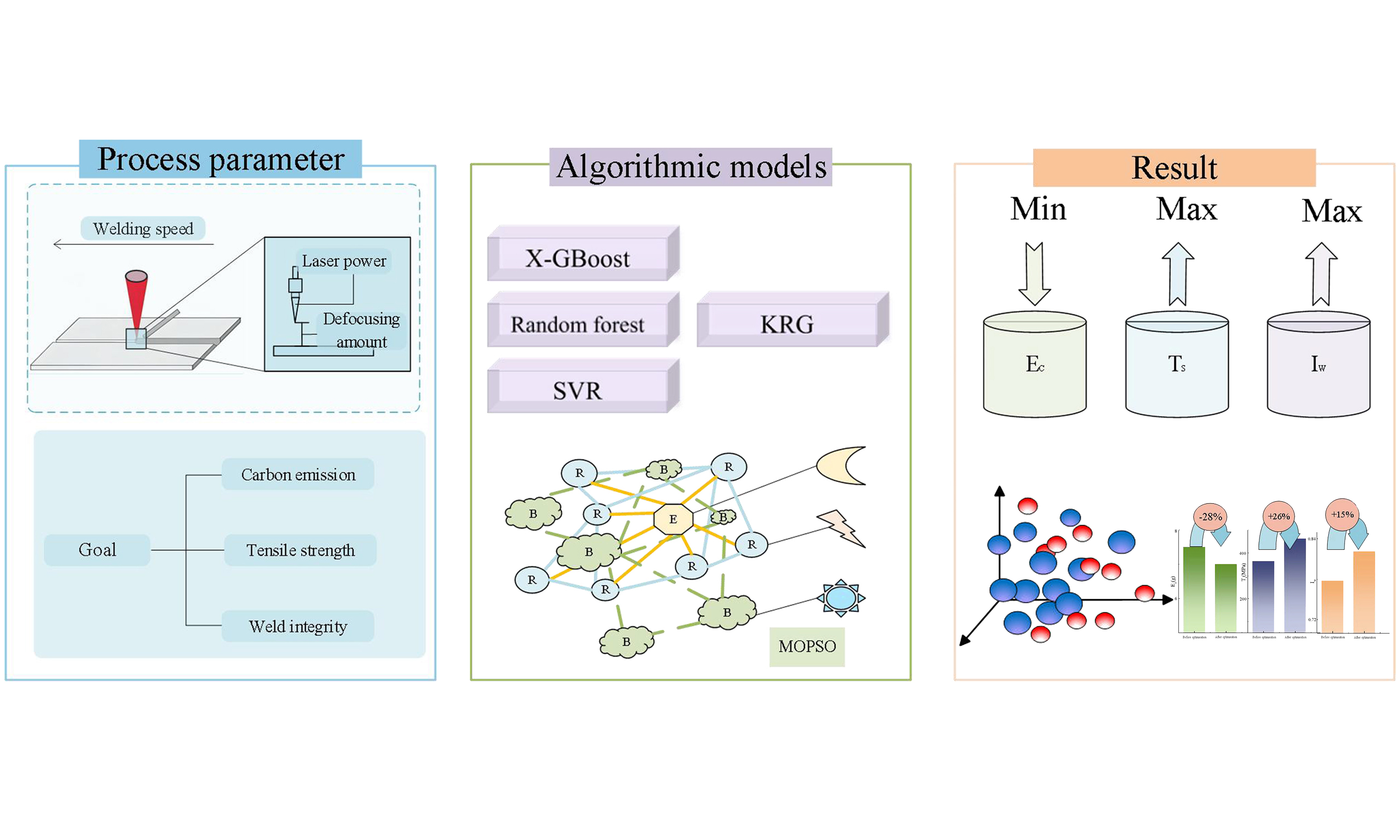
In this context, this paper proposes a hybrid method based on stacked regression and MOPSO, which aims to construct high-precision prediction models and achieve effective optimization of multi-objective performance. Stacked regression models improve their predictive accuracy and robustness by integrating multiple machine learning algorithms [such as random forest (RF), extreme gradient boosting (XGBoost), and support vector regression (SVR)] to take advantage of the strengths of different algorithms. At the same time, KRG, as a metamodel, exhibits strong generalization ability when handling small samples and high-dimensional, complex problems, further enhancing the performance of the stacked regression model. In the optimization stage, the MOPSO algorithm is introduced. Through global search and the construction of a Pareto optimal solution set, the balance between different optimization objectives can be achieved, which provides a reference for the actual process parameter design. In addition, in order to explain the predictive decision-making process of complex machine learning models, local interpretable model-agnostic explanations (LIME) and partial dependence plot (PDP) were combined to interpret and analyze the stacked models. LIME does not rely on the specific model structure, and can reveal the impact of key input features on the prediction results, providing intuitive and credible explanations for decision makers. This process not only helps verify the reliability of the model, but also provides guidance for optimizing the design. The specific flowchart is shown in Figure 1.
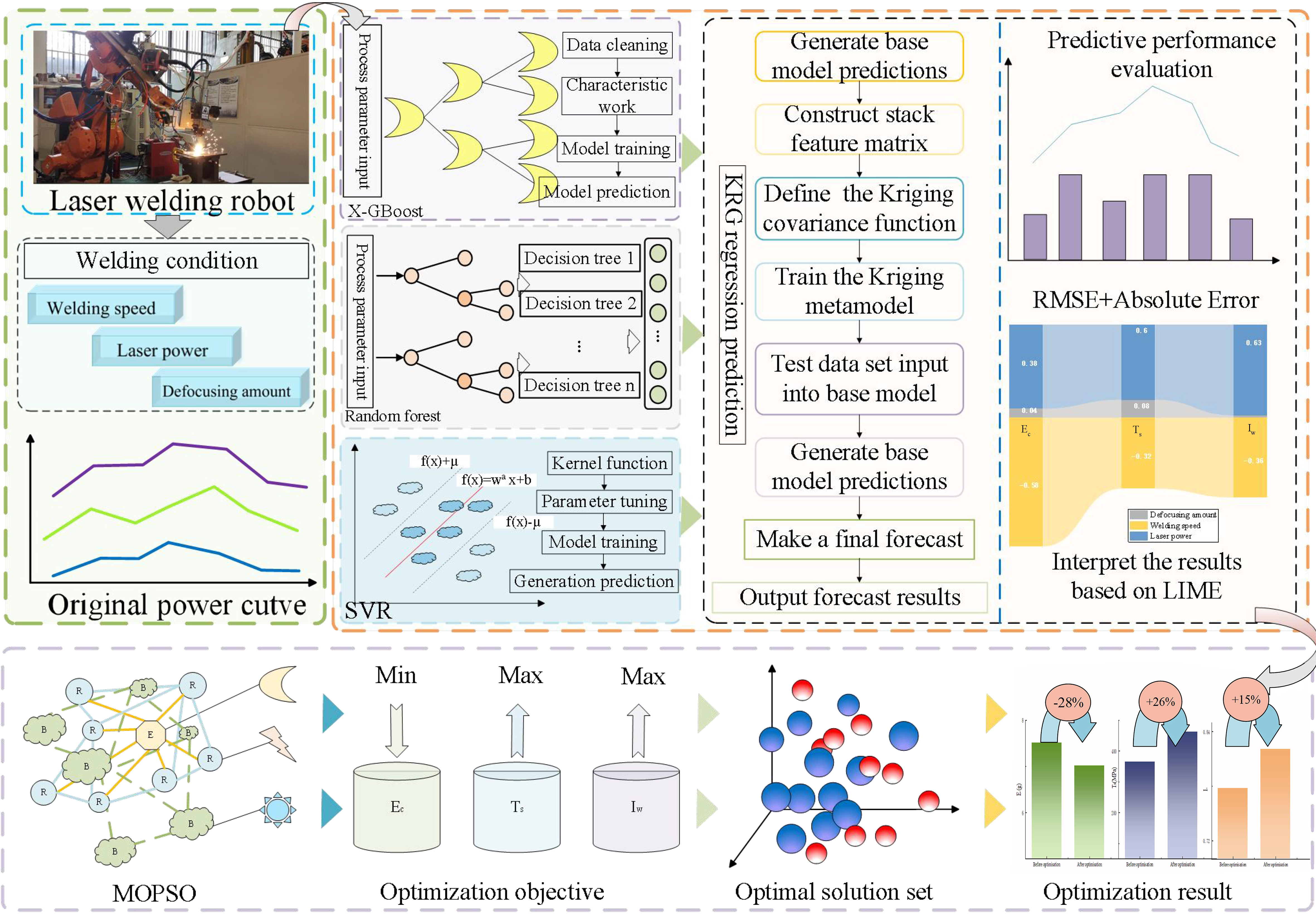
Figure 1. Optimization flowchart (Photograph taken by the authors). XGBoost: Extreme gradient boosting; SVR: support vector regression; RMSE: root mean square error; LIME: local interpretable model-agnostic explanations; MOPSO: multi-objective particle swarm optimization; EC: carbon emissions; TS: tensile strength; IW: weld depth-to-width ratio.
MATERIALS AND METHODS
Carbon emission modeling
In this study, we developed a carbon emission measurement system, as well as a calculation and conversion program for the conversion of electrical energy consumption into carbon emissions. The electric power of the platform is measured in real time, and the energy consumption of the platform is calculated by the curve integral method. As shown in Figure 2, it is the measured energy consumption of each device. The fiber laser welding platform is composed of multiple systems, and the processing process is accompanied by the generation of multi-source carbon emissions. Specifically, the energy consumption can be categorized into the laser generator, refrigeration, robotic, and auxiliary systems.
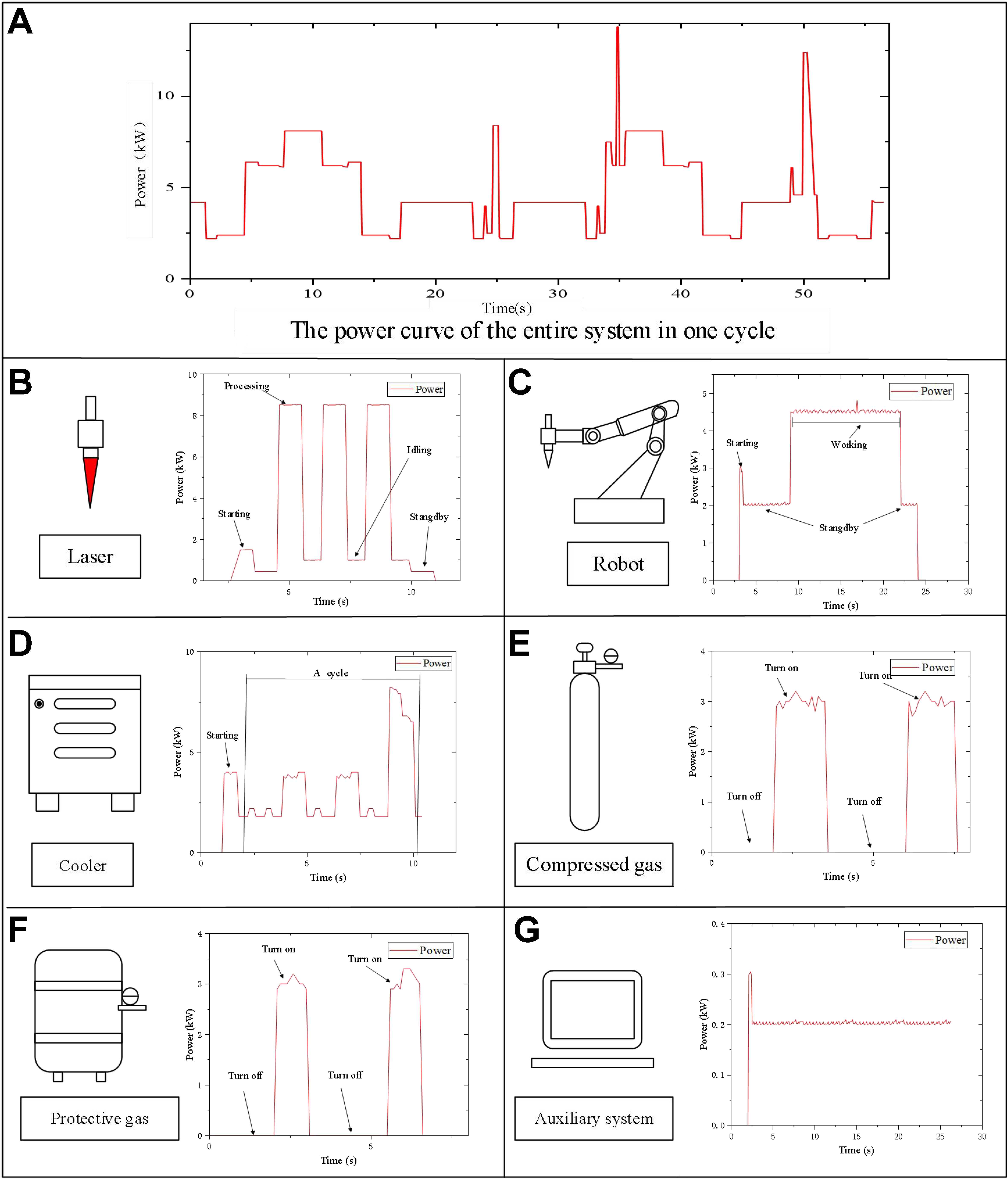
Figure 2. Power consumption diagram of laser welding system. (A) The power curve of the entire system in one cycle; (B) Power curve of the laser within one cycle; (C) Power curve of the robot within one cycle; (D) Power curve of the cooler within one cycle; (E) Power curve of the compressed gas device within one cycle; (F) Power curve of the protective gas device within one cycle; (G) Power curve of the auxiliary system within one cycle.
The power-carbon emission conversion for laser welding can be expressed as:
where CEFelec and CEFgas are carbon emission coefficients of electric energy and gas, respectively. The carbon emission factor CEFelec of electric energy consumption is 0.6747 kgCO2-ep/kWh[14]. The carbon emission factor CEFgas of protects the gas consumption is 0.9576 kgCO2-ep/m3. Elaser, Erobot, Ecool, and Eother represent laser power consumption, robot power consumption, chiller power consumption, and other energy consumption, respectively. Egas and Ecg are the volume consumption of the protective gas and the volume consumption of the compressed gas, respectively.
Tensile strength modeling
Laser process parameters will directly affect the quality of welded joints. In engineering and testing, TS is widely used in the evaluation of welding performance, which is calculated as follows:
where Fmax is the maximum bearing tension of the welded joint, and A is the cross-sectional area of the stretched sample. In addition, IW is closely related to TS and weld quality. The tensile sample was prepared according to the GB/T 2651-2008 standard (Tensile Test Method for Welded Joints). The welded workpiece was sectioned by wire cutting, and the specific sample dimensions are shown in Figure 3.
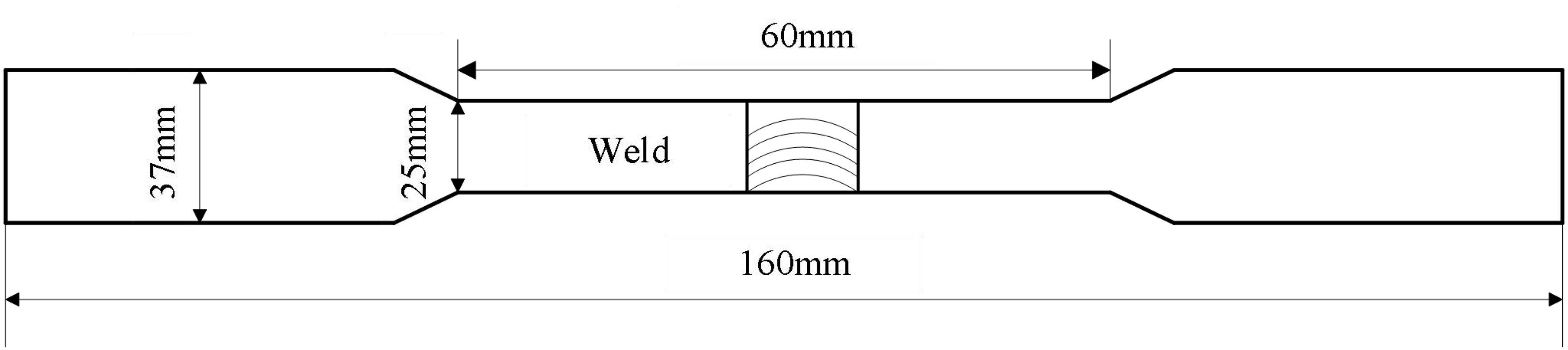
Figure 3. 316L stainless steel base metal.
Depth-to-width ratio modeling
Figure 4 shows a schematic diagram of the weld morphology in laser welding. As a key visual evaluation indicator, weld morphology is widely used for evaluating and judging welding quality. Compared with mechanical performance testing methods such as tensile testing, judging welding quality through weld morphology is not only more efficient, but also significantly reduces costs. The ideal weld seam shape needs to balance narrow width and large penetration depth. Specifically, when the penetration depth is the same, a narrower weld width helps reduce the range of the heat-affected zone, thereby reducing stress concentration and angular deformation phenomena. In the case of consistent weld width, a greater penetration depth is more advantageous in engineering practice, which is also one of the core advantages of fiber laser welding. Therefore, for weld morphology, the ideal aspect ratio is usually large, and this parameter is often used as an important indicator to measure welding quality in relevant literature. The aspect ratio (IW) of welds can be used to quantify and compare the morphological characteristics under different welding conditions, which is calculated using
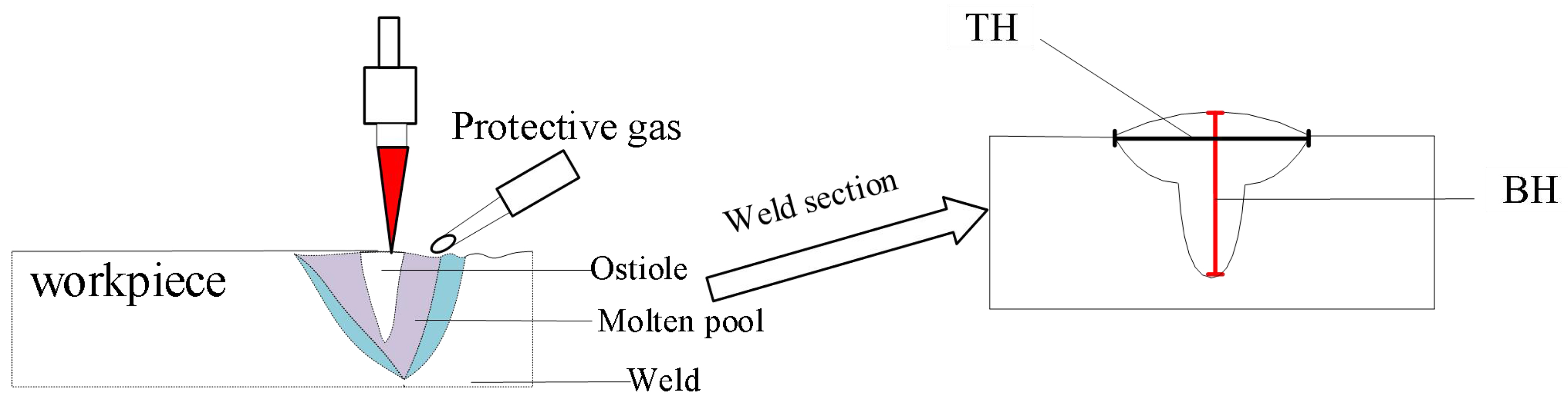
Figure 4. Definition of weld depth and height. TH: Width of weld seam on the surface of the workpiece; BH: depth of weld seam along the vertical direction.
where TH is the width of weld seam on the surface of the workpiece, and BH is depth of weld seam along the vertical direction.
Experimental design
The experimental study focused on 316L austenitic stainless steel, a material widely used in automotive and medical industries due to its superior corrosion resistance and weldability. The workpieces, with dimensions of 100 mm × 80 mm × 3 mm, underwent pre-welding preparation, including surface polishing and cleaning with anhydrous ethanol to remove oxides and contaminants. Post-welding, specimens were sectioned via wire-cutting, metallurgically mounted, and etched (HCl + HNO3 + H2O) for microstructural analysis.
All welding trials were conducted on an automated platform comprising an IPG YLR-4000 fiber laser (IPG Photonics, Oxford, MA, USA) integrated with an ABB IRB4400 robotic arm (ABB Robotics, Zürich, Switzerland) for stable path control. Argon shielding was applied at 25 L/min through an inclined nozzle. Three governing parameters - laser power (LP), welding speed (WS), and defocus distance (DA) - were selected because they jointly capture the essential balance between weld quality and EC. Specifically, laser power dictates the total energy delivered to the weld pool, directly affecting penetration depth, fusion stability, and overall energy consumption. Welding speed controls the interaction time between the beam and the material, influencing heat input per unit length, solidification rate, and consequently TS and emission levels. Defocus distance modifies the effective spot size and energy density distribution, which determines bead morphology, stability, and the IW of the weld. By varying these parameters, it is possible to explore a wide design space that reflects the practical trade-off between mechanical performance and sustainability objectives. The experimental design employed optimal Latin hypercube sampling (OLHS) to generate 25 representative parameter sets, and the platform configuration is shown in Figure 5.
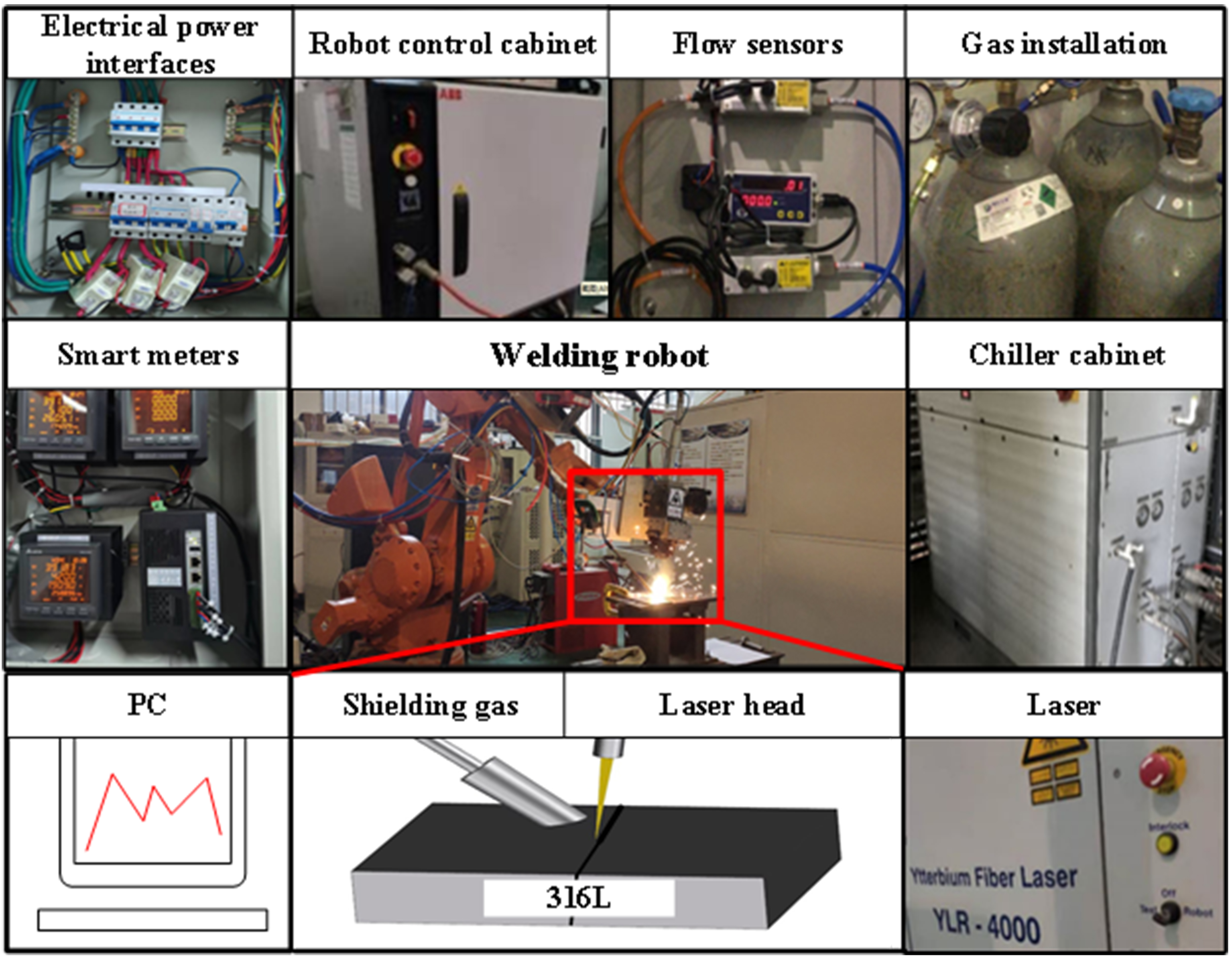
Figure 5. Fiber laser welding experimental platform (Photographs taken by the authors). PC: Personal computer.
To efficiently explore the parameter space, an OLHS method was employed[15-17]. This approach ensured uniform coverage of the design space with minimal experimental runs, reducing costs while maximizing data representativeness. Parameter range settings are shown in Table 1.
Process parameter ranges
| Parameter | Scale |
| LP/kW | 1.0-2.0 |
| WS/(m/min) | 2.4-3.6 |
| DA/mm | -2.0-0.0 |
A total of 25 experimental runs were conducted [Table 2], with responses measured for EC, TS, and IW.
The experimental data
| Item | LP/kW | WS/(m/min) | DA/mm | EC/g | Ts/MPa | Iw |
| 1 | 1.352 | 3.456 | 0 | 7.105 | 272 | 1.740 |
| 2 | 1.568 | 2.880 | -2 | 7.586 | 385 | 1.598 |
| 3 | 1.784 | 3.072 | -1 | 7.678 | 437 | 1.778 |
| 4 | 2.000 | 3.408 | -1 | 7.655 | 511 | 1.739 |
| 5 | 1.856 | 2.736 | 0 | 7.042 | 463 | 1.565 |
| 6 | 1.676 | 3.600 | -2 | 7.049 | 296 | 1.931 |
| 7 | 1.460 | 3.264 | -1 | 7.109 | 298 | 1.601 |
| 8 | 1.892 | 2.640 | -1 | 8.041 | 461 | 1.836 |
| 9 | 1.244 | 2.544 | -1 | 7.707 | 309 | 1.350 |
| 10 | 1.208 | 2.928 | -2 | 7.299 | 280 | 1.393 |
| 11 | 1.316 | 2.592 | -1 | 7.717 | 296 | 1.712 |
| 12 | 1.748 | 3.552 | -1 | 7.116 | 387 | 1.861 |
| 13 | 1.712 | 2.448 | -1 | 8.260 | 460 | 1.711 |
| 14 | 1.424 | 3.312 | -2 | 7.060 | 297 | 1.571 |
| 15 | 1.964 | 3.168 | 0 | 7.672 | 403 | 1.551 |
| 16 | 1.820 | 3.216 | -2 | 7.433 | 349 | 1.871 |
| 17 | 1.532 | 2.832 | -1 | 7.598 | 417 | 1.547 |
| 18 | 1.136 | 3.360 | -1 | 6.930 | 283 | 1.465 |
| 19 | 1.640 | 3.120 | 0 | 7.549 | 372 | 1.964 |
| 20 | 1.928 | 2.784 | -2 | 8.041 | 424 | 1.760 |
| 21 | 1.388 | 2.496 | -2 | 7.796 | 324 | 1.484 |
| 22 | 1.280 | 3.024 | 0 | 7.353 | 272 | 1.785 |
| 23 | 1.604 | 2.400 | -1 | 8.093 | 466 | 1.745 |
| 24 | 1.496 | 2.688 | 0 | 7.771 | 381 | 1.550 |
| 25 | 1.172 | 2.976 | -1 | 7.107 | 279 | 1.469 |
Stack process description
The proposed stacked regression model integrates heterogeneous base learners (RF, XGBoost, and SVR) with a KRG meta-model to leverage complementary learning patterns and enhance generalization. As illustrated in Figure 6, the model follows a two-stage hierarchical structure.
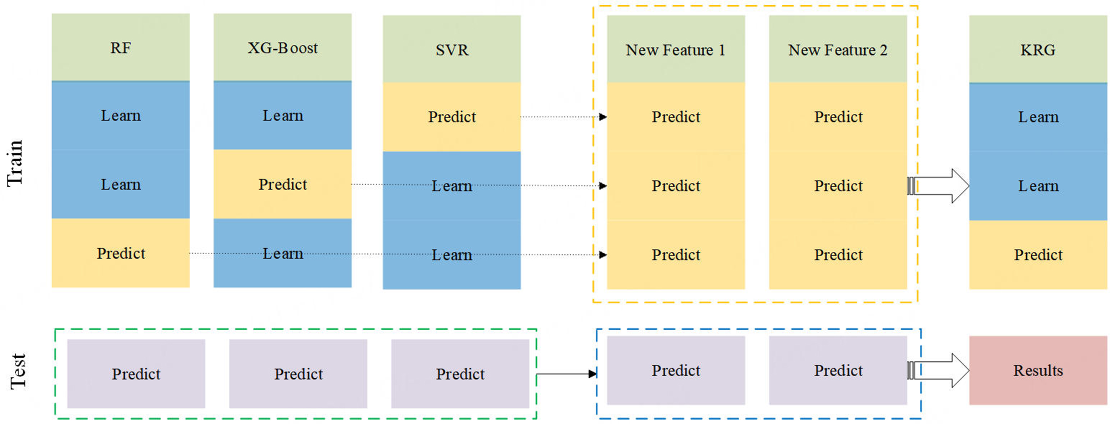
Figure 6. Stacked regression model structure. RF: Random forest; XGBoost: extreme gradient boosting; SVR: support vector regression; KRG: Kriging.
In this study, a stacking framework was constructed to improve predictive accuracy and robustness for laser welding process modeling. The main role of the base models is to generate preliminary predictions for each target variable, which are then input into the meta-model as new features for further optimization and correction. The base models selected include RF, XGBoost, and SVR[17,18]. These algorithms were chosen due to their complementary learning strategies: RF, as a bagging-based ensemble of decision trees, is robust to noise and captures nonlinear feature interactions; XGBoost, a boosting-based method, excels in modeling complex dependencies and has demonstrated superior accuracy in structured data[19-21]; SVR leverages kernel functions to capture nonlinear patterns and maintains strong generalization even under limited samples. The meta-model employs KRG, a Gaussian process regression method, which provides smoother and more generalized outputs by exploiting the spatial correlation among the predictions of the base learners[22,23]. Unlike a simple concatenation of outputs, the stacking process integrates the complementary strengths of the base models and the meta-model through a hierarchical learning mechanism. By feeding the outputs of the base models as inputs to KRG, the framework achieves higher-level integration, yielding final predictions that are both more accurate and more reliable. This design leverages the diversity of the base models and the interpolation capability of the meta-model, thereby enhancing the robustness and generalization of the predictive system compared with any single-model approach.
Using the experimental equipment mentioned earlier to supplement 200 sets of experimental data, 150 sets were randomly selected as the training set to train the basic model (RF, XGBoost, SVR) and KRG meta model, while the remaining 50 sets were used as independent test sets to evaluate the predictive performance of the model. The division of the training and testing sets is stratified according to parameter distribution, ensuring that the two groups maintain consistent statistical characteristics in terms of LP, WS, DA range and output response distribution to avoid model evaluation bias caused by uneven data distribution.
The implementation of the stack model is divided into the following steps:
Step 1: Base model training: Three base models - RF, XGBoost and SVR - were trained using training dataset 1 and target output 2. The prediction result zj(i) of the JTH base model fj for sample Xi is obtained as:
zj(i): Prediction result of the j-th base model for the i-th sample; Xi: The i-th input sample; j: Index of the base model, taking values of 1, 2, 3; i: Index of the sample.
Step 2: Base model prediction: The base models are used to generate prediction results on both the training and test sets. The prediction results from the training set are then concatenated to form a new feature matrix Z. The new feature matrix is constructed as follows:
Step 3: With Z as the input and Y as the output, the KRG meta-model is trained. The prediction of the meta-model is given by:
where fKRG is the KRG model.
Step 4: The prediction results of the base model on the test set constitute Y1, and the meta-model predicts Y2 to get the final predicted value of the target variable.
The algorithm flowchart is given in Figure 7.
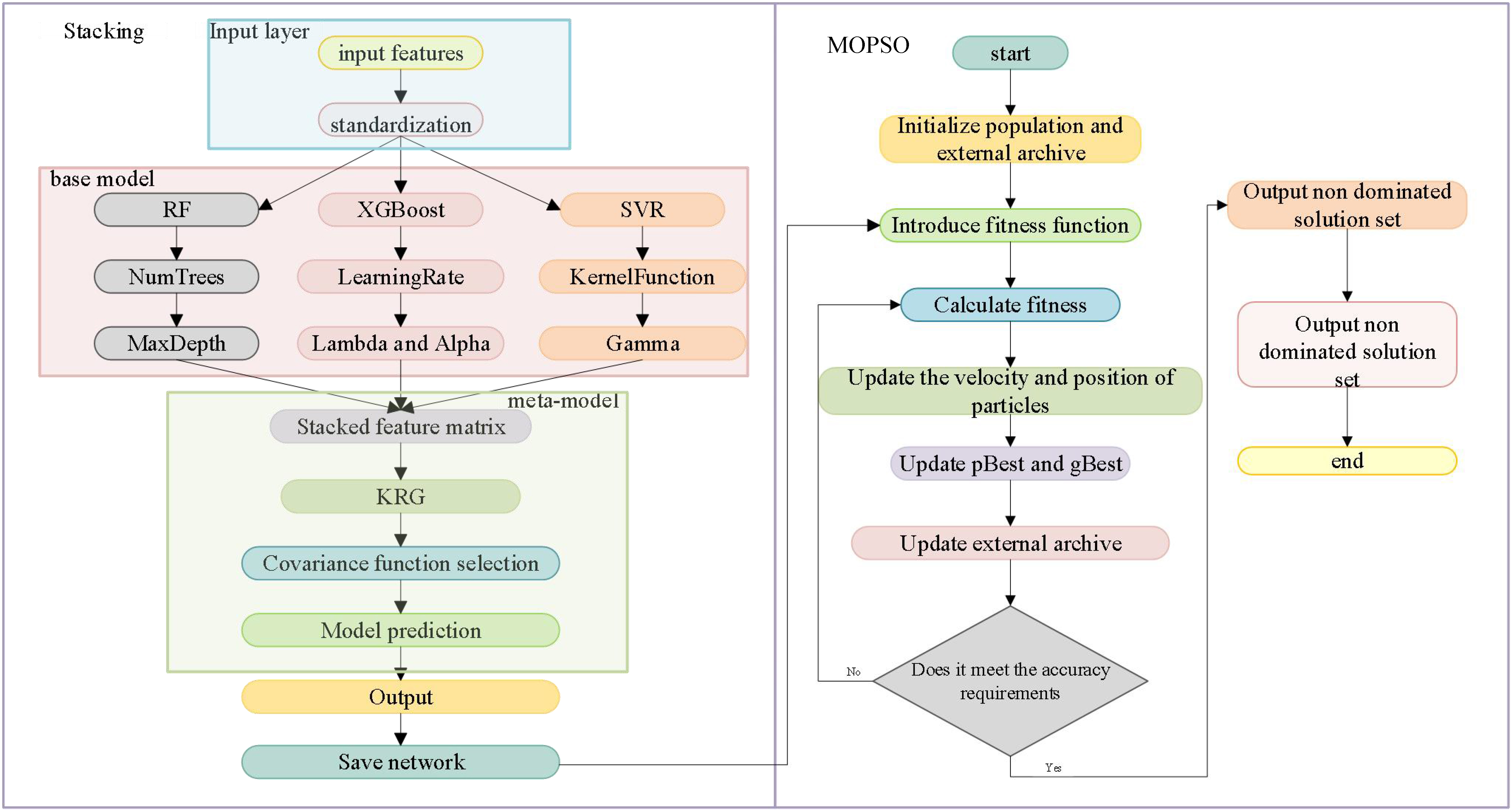
Figure 7. Algorithm flowchart. RF: Random forest; XGBoost: extreme gradient boosting; SVR: support vector regression; KRG: Kriging; MOPSO: multi-objective particle swarm optimization.
To enable the model to more effectively capture the relationship between input features and output targets, improve training efficiency, and eliminate dimensional discrepancies, the data are normalized using
where x is a data point in the original dataset, xmin and xmax are the minimum and maximum values of the feature, respectively, and xnew is the normalized value. This procedure scales all data to the interval [0, 1], making features comparable and preventing performance issues caused by large differences in data scales in certain machine learning algorithms.
RF: Optimal hyperparameters (n_estimators = 200, max_depth = 8) were determined via grid search to balance model complexity and computational efficiency.
XGBoost: Bayesian optimization determined the optimal hyperparameters - learning rate (0.05), maximum tree depth (5), and L2 regularization (λ = 0.1) - to minimize the validation root mean square error (RMSE).
SVR: Cross-validation selected the radial basis function (RBF) kernel parameters - C = 1 and γ = “scale” - to ensure robust generalization in high-dimensional feature spaces.
KRG: A Matérn kernel (ν = 1.5) was used to model the spatial correlations among the base model predictions:
where r is the Euclidean distance between input points (or distance in the parameter space), σ2 is the signal variance controlling the amplitude of the function, and l is the length-scale parameter determining the decay rate of correlation.
Hyperparameters were optimized using 10 restarts of maximum likelihood estimation (MLE) to reduce the risk of convergence to local minima.
Optimization model
The MOPSO algorithm is an extension of the traditional particle swarm optimization (PSO) method, designed to handle multiple conflicting objectives simultaneously. The MOPSO algorithm is an extension of the traditional PSO method, designed to handle multiple conflicting objectives simultaneously[24,25]. While classical PSO is limited to optimizing a single target function, MOPSO enables the discovery of one or more non-dominated solutions under multi-objective conditions, thus providing a well-distributed Pareto front. Its fundamental principle is to simulate the social behavior and motion dynamics of particle populations in the search space, where each particle represents a candidate solution corresponding to a specific combination of process parameters[26,27]. The algorithm begins by initializing a population of particles within the design space. Each particle is evaluated using the defined fitness functions, which in this study are EC, TS, and IW. During the iterative process, particles update their velocities and positions based on both their individual best solutions (pBest) and the global best solutions (gBest). At the same time, an external archive is maintained to store the current non-dominated solutions, while leader selection and crowding distance mechanisms are applied to preserve population diversity and guide the swarm toward convergence. Through this iterative mechanism, MOPSO gradually evolves the particle population toward the Pareto front, achieving a balanced optimization among multiple objectives. The overall workflow of the algorithm, including initialization, evaluation, update, and archive management, is illustrated in Figure 7.
RESULTS AND DISCUSSION
Analysis of test results
To further evaluate the relative influence of process parameters on the response variables, analysis of variance (ANOVA) was performed. The sum of squares (SS) for each factor (laser power, welding speed, and defocusing distance) was calculated based on the deviations between the mean response at each factor level and the overall mean response. The mean square (MS) values were obtained by dividing SS by the corresponding degrees of freedom (DF), and the F-values were calculated to determine statistical significance. The contribution ratio of each factor was then derived as:
where SSfactor represents the variation attributed to a given process parameter, and SStotal is the total variation in the model. This method quantitatively reflects the proportion of variability explained by each parameter, with higher ratios indicating greater influence on the response. All statistical analyses were carried out using Minitab 19 software to ensure accuracy and reproducibility.
To systematically evaluate the influence of laser welding parameters on EC, TS, and IW, ANOVA and main effect analysis were conducted[28,29]. The ANOVA results [Table 3] quantify the contribution of each process parameter (laser power, welding speed, and defocusing distance) to the three response indicators, while the main effect plots [Figure 8] visualize the trends of parameter impacts.
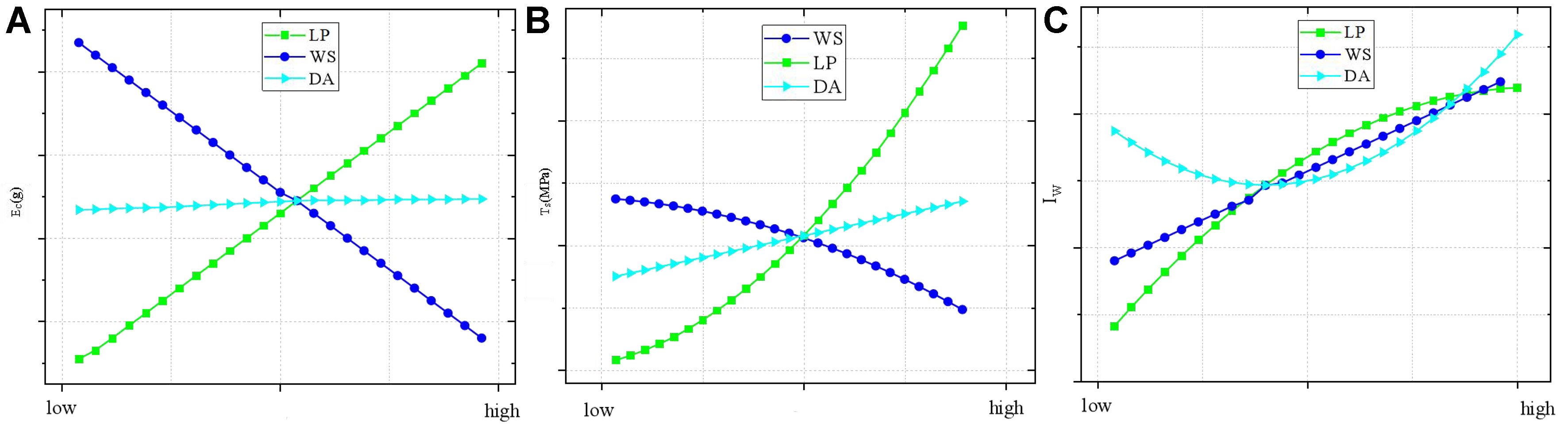
Figure 8. Main effects plot for response indicators. (A) Main effect analysis of EC; (B) Main effect analysis of TS; (C) Main effect analysis of IW. EC: Carbon emissions; TS: tensile strength; IW: weld depth-to-width ratio; LP: laser power; WS: welding speed; DA: defocus distance.
ANOVA on the output responses
| Output responses | Technological parameter | Contribution/% |
| EC/g | LP/kw | 32.5 |
| WS/(m/min) | 55.4 | |
| DA/mm | 12.1 | |
| TS/MPa | LP/kw | 68.5 |
| WS/(m/min) | 27.1 | |
| DA/mm | 4.4 | |
| IW | LP/kw | 45.2 |
| WS/(m/min) | 38.3 | |
| DA/mm | 16.5 |
As shown in Table 3, WS exhibits the highest contribution (55.4%) to EC, followed by laser power (LP, 32.5%) and defocusing distance (DA, 12.1%). This indicates that WS is the most critical factor in controlling energy consumption and EC. For TS, LP dominates with a 68.5% contribution, significantly surpassing WS (27.1%) and DA (5.1%), highlighting the decisive role of laser energy input in enhancing joint strength. In contrast, Iw is influenced more evenly by LP (45.2%) and WS (38.3%), with DA contributing moderately (16.5%), suggesting that weld geometry and integrity require a balanced adjustment of energy input and processing speed.
By ANOVA, the main effect of a factor on the response is reflected by the mean difference between its levels. The main effect of each process parameter on the three response indicators is analyzed in Figure 8, where the abscissa indicates the different levels of the parameter. In Figure 8A, EC from electrical energy consumption increases and decreases monotonically with increasing laser power and welding speed, respectively, while changes in defocusing distance have little effect. In Figure 8B, the IW shows a significant upward trend with increasing laser power, similar to the influence of welding speed. When defocusing distance varies, the weld IW first decreases and then increases. In Figure 8C, increasing laser power effectively raises TS, whereas increasing welding speed significantly decreases it, and defocusing distance has a minor effect.
The combined ANOVA and main effect analysis demonstrate a clear trade-off between process parameters:
1. Increasing WS reduces EC but compromises TS and IW.
2. Elevating LP enhances TS and IW at the cost of higher EC.
3. Adjusting DA offers limited optimization flexibility, primarily affecting IW.
Performance of the stacking prediction model
A total of 200 datasets were used for training and testing, with five-fold cross-validation performed on the testing set. The parameter settings are summarized in Table 4, and the prediction results are presented in Table 5 and Figure 9.
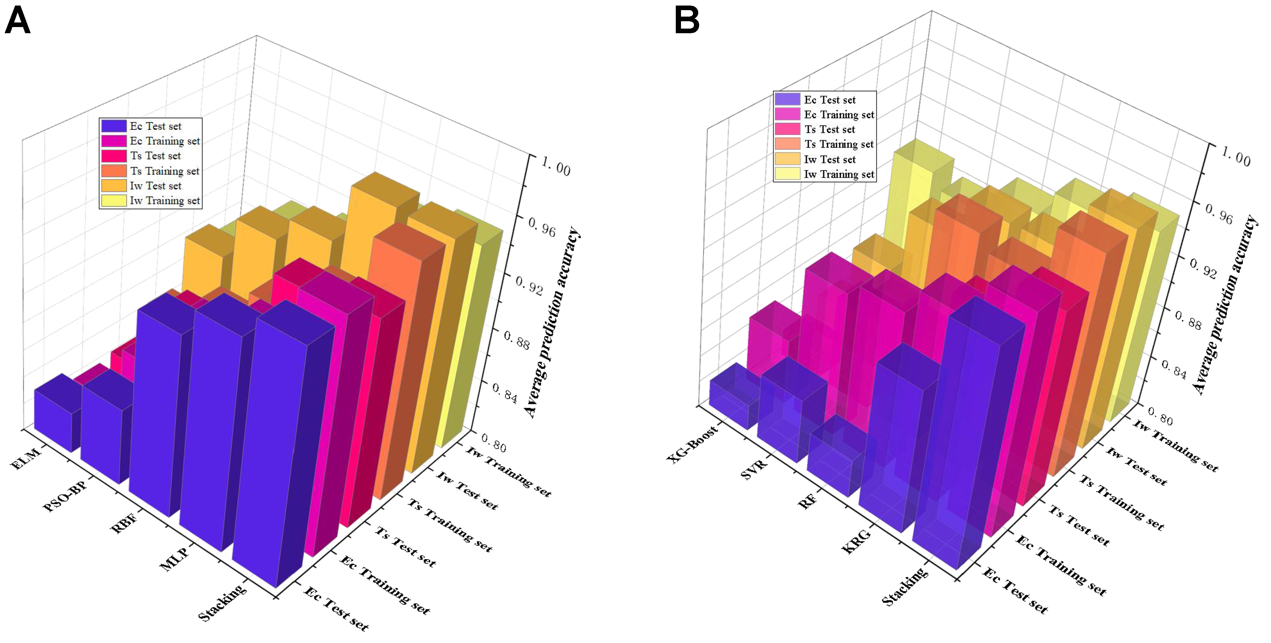
Figure 9. Five-fold cross-validation average prediction accuracy. (A) Comparison of prediction results between the Stacking model and other common proxy models; (B) Comparison of prediction results among the Stacking model, the base models, and the meta-model. EC: Carbon emissions; TS: tensile strength; IW: weld depth-to-width ratio; ELM: extreme learning machine; PSO-BP: particle swarm optimization - back propagation; RBF: radial basis function; MLP: multi-layer perceptron; XGBoost: extreme gradient boosting; SVR: support vector regression; RF: random forest; KRG: Kriging.
Key parameters of the algorithm
| Model | Key parameter | Set point |
| RF | n_estimators, max_depth | 200, 8 |
| XGBoost | learning_rate, max_depth | 0.05, 5 |
| SVR | C, γ | 1, 'scale' |
| KRG | kernel, n_restarts | Matérn (ν = 1.5), 10 |
Average results of 5-fold cross-validation error
| Model | EC (RMSE) | TS (RMSE) | IW (RMSE) | R2 |
| Stacked model | 0.0121 | 0.0102 | 0.0143 | 0.971 |
| RF | 0.0324 | 0.0465 | 0.0258 | 0.874 |
| XGBoost | 0.0514 | 0.0254 | 0.0632 | 0.872 |
| SVR | 0.0337 | 0.0497 | 0.0471 | 0.931 |
| MLP | 0.0224 | 0.0311 | 0.0302 | 0.892 |
| RBF | 0.0304 | 0.0504 | 0.0337 | 0.878 |
| PSO-BP | 0.0428 | 0.0453 | 0.0417 | 0.853 |
| ELM | 0.0403 | 0.0331 | 0.0544 | 0.842 |
Figure 9 and Table 5 present the results of five-fold cross-validation, which clearly demonstrate the superior performance of the stacked model. The consistently high coefficient of determination (R2) values across folds indicate that the stacked model effectively captures the complex relationships between process parameters and output responses, while the relatively low RMSE highlights its precision in prediction. Moreover, the stacked model integrates multiple base learners - RF, XGBoost, and SVR - with a KRG meta-model, enabling the effective combination of the complementary strengths of each base algorithm[30,31]. This integration enhances the model’s capacity to manage non-linear relationships and high-dimensional data, thereby improving both predictive accuracy and robustness. Compared with traditional regression models, such as linear regression, and individual base learners, the stacked framework achieves significant improvements in accuracy and generalization. The results of five-fold cross-validation further validate the reliability of the stacked model across different data partitions, reinforcing its superiority over single-model approaches.
To further evaluate the robustness and generalization of the proposed stacked model, a noise robustness test was conducted, as shown in Figure 10. Gaussian noise with amplitudes of ±3% and ±5% was added to the input parameters (laser power, welding speed, and defocus distance). The results show that the model consistently maintained high predictive performance, with all R2 values remaining above 0.95 and RMSE exhibiting only minor increases relative to the noise-free baseline. These outcomes demonstrate that the stacked model is not overly sensitive to small input perturbations, confirming its stability and reliability in handling realistic variability in process data while maintaining strong predictive accuracy.
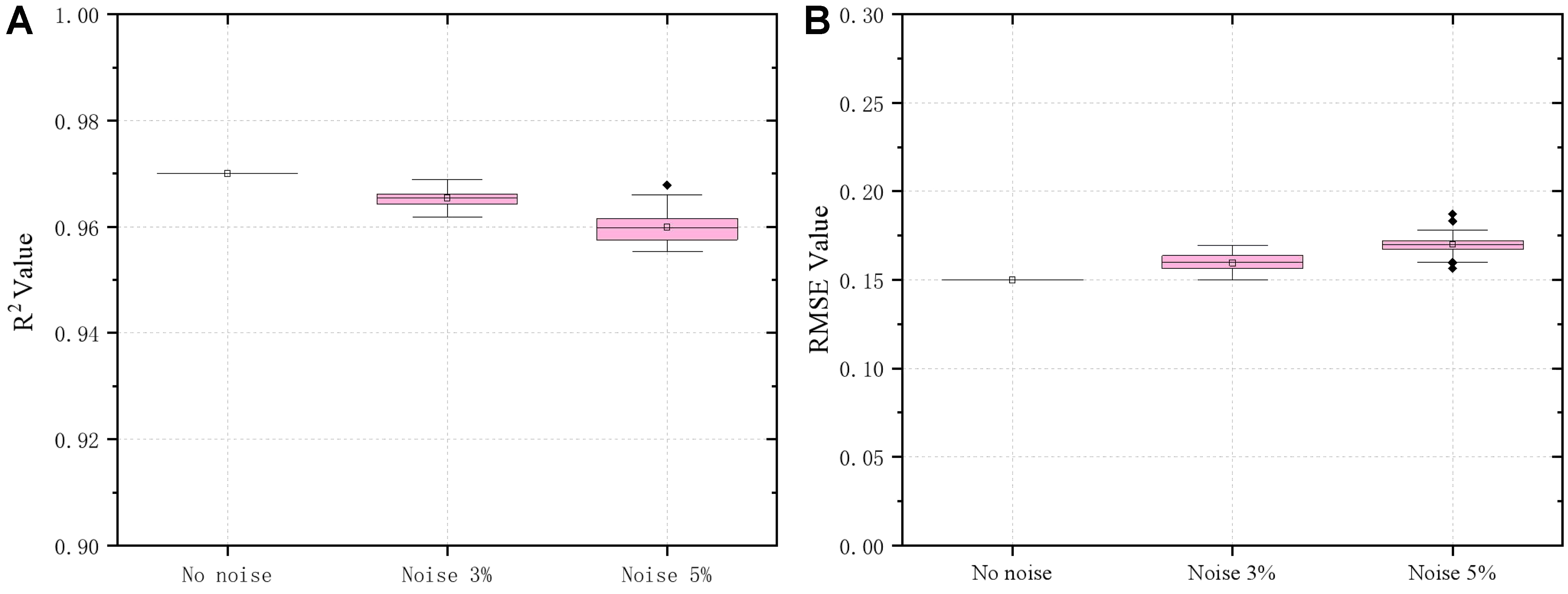
Figure 10. Results of the noise robustness test for the Stacking model. (A) R2 value; (B) RMSE value. R2: Coefficient of determination; RMSE: root mean square error.
Model interpretation
LIME explains the individual prediction results of stacked regression models by constructing locally interpretable surrogate models. The specific process is as follows: Firstly, 2,000 Gaussian perturbation samples are generated within the feature space neighborhood of the target sample point to form a local dataset. The disturbance range is determined by adaptive kernel width, ensuring neighborhood coverage and feature dimension adaptation. Subsequently, the trained stacking model is used to predict the EC, TS, and weld depth to width ratio (IW) output values of the perturbed samples, and similarity weights are calculated using an exponential kernel function [wx = exp(-||x - x′||2/σ2)] (wx: Similarity weight of the Gaussian perturbed sample relative to the target sample; x: Target sample vector in the feature space; x′: Gaussian perturbed sample vector in the neighborhood of target sample x; σ2: Square of the adaptive kernel widt). Based on this weighted dataset, train a ridge regression model (Regularization coefficient α = 0.02) as a local surrogate model, and the linear coefficient is the feature importance weight. The process is implemented by calling the Lime library (v0.2.0.1) in the Python 3.9 environment, Parameter selection has been verified by Monte Carlo simulation: when the number of perturbed samples N > 3,000, the standard deviation of feature weights converges to within 0.1, meeting the engineering confidence requirements[32].
To elucidate the decision-making mechanism of the stacked regression model, LIME was employed to quantify the feature-specific contributions to predictions. LIME approximates the model’s behavior locally by constructing linear surrogate models around individual predictions, enabling instance-level explanations. The normalized feature importance values for EC, TS, and IW are summarized in Figure 11.
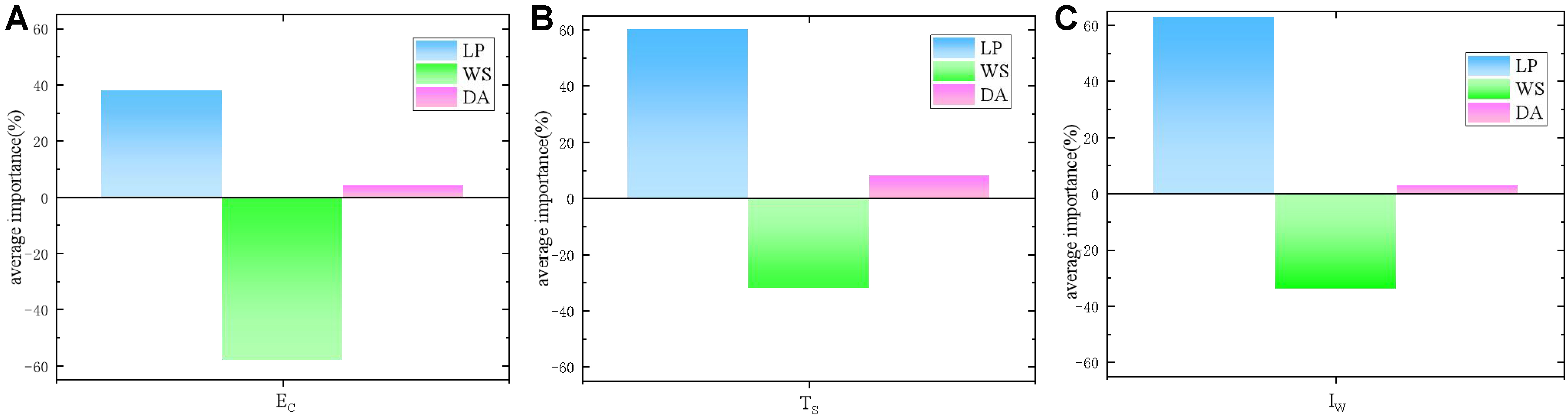
Figure 11. Average importance. (A) The average importance of EC; (B) The average importance of TS; (C) The average importance of IW. EC: Carbon emissions; TS: tensile strength; IW: weld depth-to-width ratio; LP: laser power; WS: welding speed; DA: defocus distance.
LIME analysis reveals the local impacts of laser welding parameters: WS negatively affects EC (weight = -0.58 ± 0.08), while LP has a positive link (weight = +0.38 ± 0.06). This aligns with ANOVA results showing WS (55.4%) and LP (32.5%) contributions to EC. For TS, LP has a dominant positive weight (+0.69 ± 0.05), matching its 68.5% ANOVA contribution, and WS’s negative impact (-0.31 ± 0.04) fits its 27.1% contribution. IW is jointly controlled by LP (+0.50 ± 0.07) and WS (-0.41 ± 0.06), reflecting their balanced ANOVA contributions (LP: 45.2%, WS: 38.3%). Defocusing distance (DA) has minimal influence in LIME (weight < ±0.1), consistent with its low ANOVA contributions (EC: 12.1%, TS: 5.1%, IW: 16.5%), confirming the model’s statistical robustness in both global and local interpretations.
In order to gain a more comprehensive understanding of the model’s decision-making process, this study combines LIME and PDP. LIME explains individual predictions through local surrogate models, highlighting feature contributions for specific instances. However, LIME’s focus on single data points limits its ability to capture the overall impact of features across the entire dataset. PDP complements this by visualizing the global average effect of individual features on model predictions, demonstrating how changes in feature values systematically influence model outputs. This combination ensures a thorough and multi-faceted understanding of the model, providing a robust theoretical foundation for optimizing laser welding parameters.
PDP is used to quantify the global marginal effect of a single feature on the model output. When analyzing, select the target feature (such as LP) and evenly divide it into 100 grid points within its value range (1.0-2.0 kW). To balance computational efficiency and statistical reliability of small sample data (n = 25), a conditional distribution sampling strategy is adopted: based on the joint distribution of experimental data, feature dependency relationships are modeled through kernel density estimation (KDE); Extract 100 sets of xs(k) samples from the conditional distribution P for each grid point xc; Calculate marginal effects using [
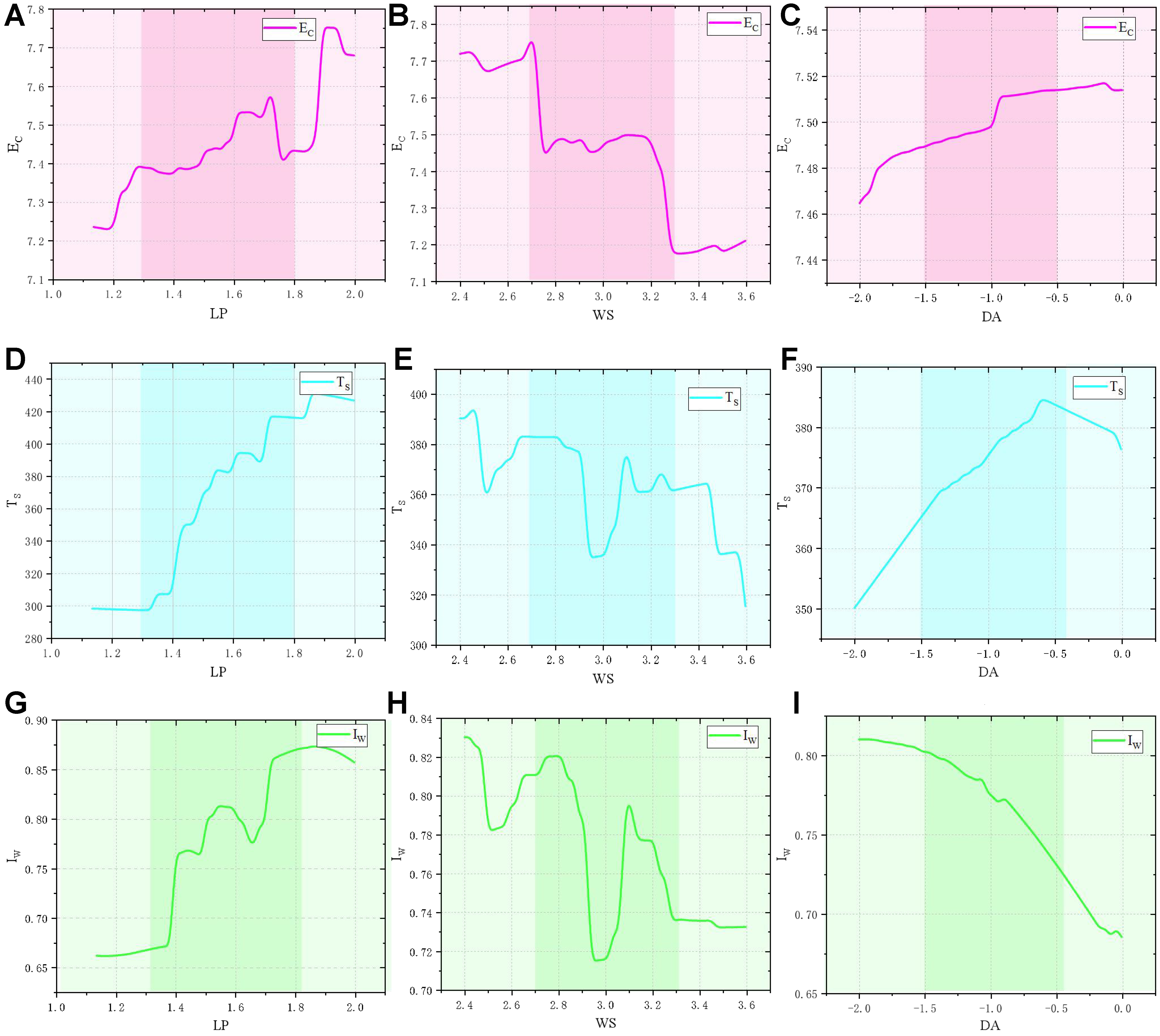
Figure 12. PDP analysis for laser welding parameters. (A) Partial dependence of EC vs. LP; (B) Partial dependence of EC vs. WS; (C) Partial dependence of EC vs. DA; (D) Partial dependence of TS vs. LP; (E) Partial dependence of TS vs. WS; (F) Partial dependence of TS vs. DA; (G) Partial dependence of IW vs. LP; (H) Partial dependence of IW vs. WS; (I) Partial dependence of IW vs. DA. PDP: Partial dependence plot; EC: carbon emissions; LP: laser power; WS: welding speed; DA: defocus distance; TS: tensile strength; IW: weld depth-to-width ratio.
PDPs analyze how variations in individual features (while keeping other features constant) affect the predicted output[33]. For instance, the PDP for EC illustrates the relationship between welding speed and EC, clearly showing that as welding speed increases, EC decreases, aligning with the insights gained from LIME. PDPs provide a more holistic view of the feature-target relationship by aggregating over all data points, thus offering a better understanding of the feature’s impact on model performance. In summary, while LIME gives local, instance-level explanations of the model’s behavior, PDPs provide global insights, aggregating the effects of features on the target variables. Together, they offer complementary perspectives: LIME helps understand individual predictions, while PDPs reveal the overall trends and interactions between process parameters and outputs, thereby enhancing the interpretability of the model.
Analysis of EC: As shown in Figure 12A and B, when the defocusing distance is maintained at a constant value, the reduction of laser power and the increase of welding speed will significantly reduce EC. This is because the increased welding speed can effectively reduce system uptime, thereby reducing energy consumption and EC. The reduction of laser power directly reduces the total input of light energy into heat energy. In addition, as shown in Figure 12B and C, when the laser power is maintained at a constant value, the change of defocusing distance has a small impact on EC, while the change of welding speed has a greater impact on EC, which shows that the greater the welding speed, the lower the EC, which further proves the critical impact of welding speed on the energy efficiency of the system. As shown in Figure 12C, when the welding speed and laser power are kept at a fixed value, the increase in the defocusing distance has a small positive effect on EC.
Analysis of TS: As shown in Figure 12D and E, both the increase of laser power and the decrease of welding speed contribute to the improvement of TS when the defocusing distance is constant. This is because the increase in laser power provides a higher energy input, which is conducive to the formation of the weld pool and deep penetration, thus improving the welding strength. At the same time, the reduction of welding speed extends the time of laser interaction with the material, and further enhances the quality of the weld pool. As shown in Figure 12E, when the laser power is maintained at a fixed value, the increase of welding speed will lead to a significant decrease in TS, which may be because the welding speed is too high, resulting in too fast cooling of the weld pool, and the complete welding structure is not fully formed. As shown in Figure 12F, when the welding speed and laser power as maintained at a constant value, the DA can further improve the TS, while the change of defocusing distance has relatively little influence on the TS.
Analysis of IW: As shown in Figure 12G and H, when the defocusing distance is maintained at a constant value, the increase of laser power and the decrease of welding speed can significantly improve the IW. This is because higher laser power can improve the depth and consistency of the weld, while lower welding speed can reduce the instability of the weld pool, thereby improving the IW of the weld. As shown in Figure 12H, when the laser power and defocusing distance are maintained at constant values, the reduction of welding speed has a particularly significant effect on the improvement of the IW, which indicates that a slower welding speed can reduce the defects generated in the welding process. As shown in Figure 12I, when the welding speed and laser power remain constant, an increase in defocusing distance significantly reduces the aspect ratio.
In summary, the combination of LIME and PDP provides a comprehensive interpretation of the model, ensuring that the optimization of laser welding parameters is guided by both local and global insights into the relationships between input parameters and output responses. This multi-faceted analysis not only enhances the model’s transparency but also ensures the robustness and reliability of the optimization outcomes.
Optimization model
The fitness function for the MOPSO algorithm is based on three RBF neural network prediction models trained collectively. The hybrid algorithm was implemented in Python with the following parameter settings: number of particle swarms p = 100, number of iterations c = 50, inertia weight w = 0.8, local velocity factor c1 = 0.1, global velocity factor c2 = 0.1, number of mesh aliquots m = 10, and external archiving threshold t = 300. This configuration represents the optimal combination of parameters we have derived after analyzing the size of the experimental data, evaluating empirical parameter suggestions found in relevant literature, and conducting multiple iterative tests. Figure 13 shows the Pareto optimal solution set and the trend between individual process parameters (horizontal coordinate) and optimization objectives (vertical coordinate).
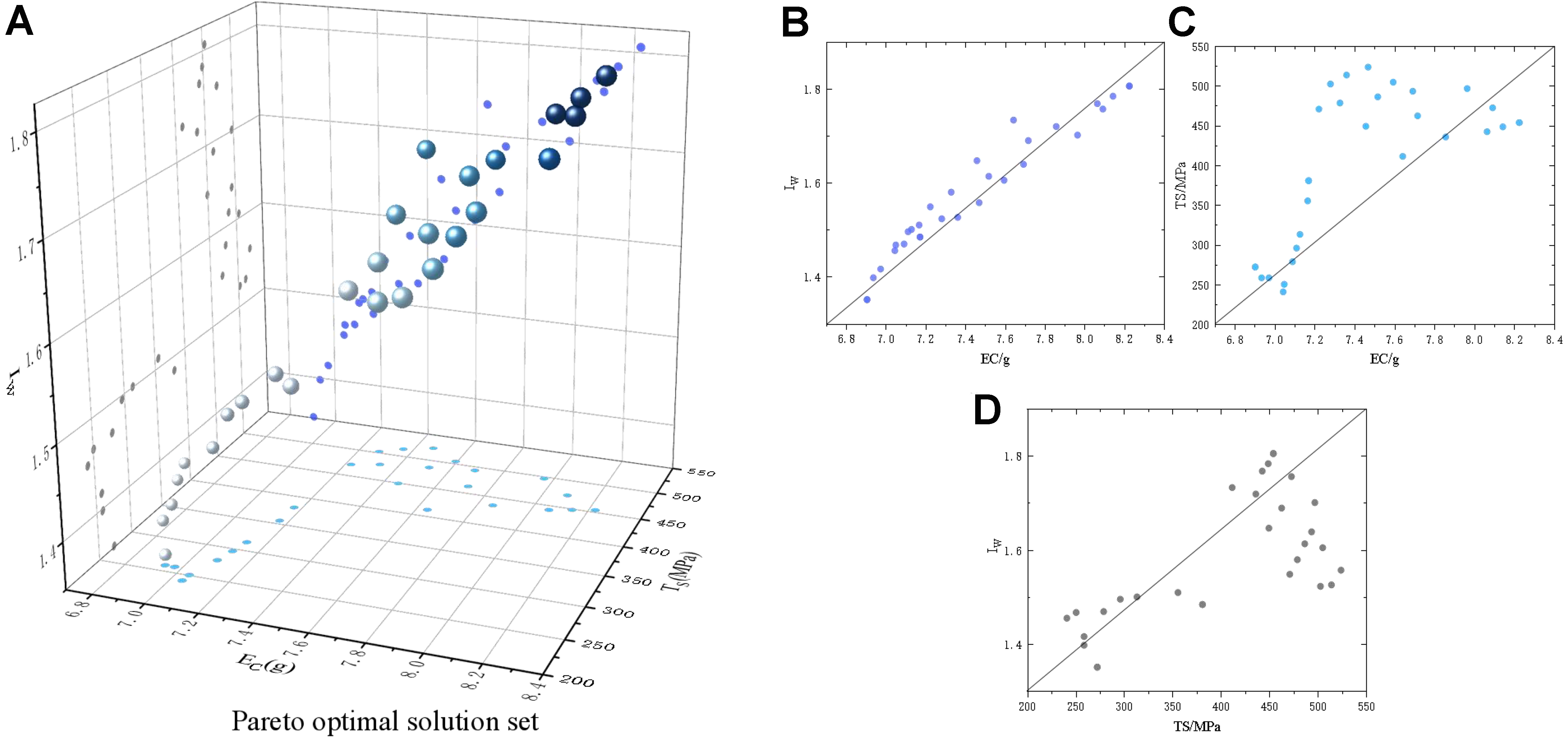
Figure 13. Pareto optimal solution set. (A) 3D Pareto solution set; (B) Mapping of Z-axis and X-axis; (C) Mapping of Y-axis and X-axis; (D) Mapping of Z-axis and Y-axis. IW: Weld depth-to-width ratio; EC: carbon emissions; TS: tensile strength.
Optimize model evaluation
To evaluate the performance of the proposed optimization framework, MOPSO was benchmarked against the NSGA-II and the decomposition-based sparrow search algorithm (SSA). Each algorithm was executed 30 times using the Deb–Thiele–Laumanns–Zitzler (DTLZ) benchmark functions DTLZ5 and DTLZ6. The hypervolume (HV) and inverted generational distance (IGD) metrics were recorded for each run, and the results were visualized through box plots, as shown in Figure 13. Larger HV values and smaller IGD values indicate better convergence and diversity of the obtained solution sets.
As illustrated in Figure 14, the MOPSO algorithm consistently outperformed the other two methods in terms of both HV and IGD. This indicates that the solution set generated by MOPSO is closer to the true Pareto front, reflecting superior convergence and distribution characteristics. Consequently, the overall performance of the proposed MOPSO optimization model is demonstrated to be highly effective in balancing convergence and diversity.
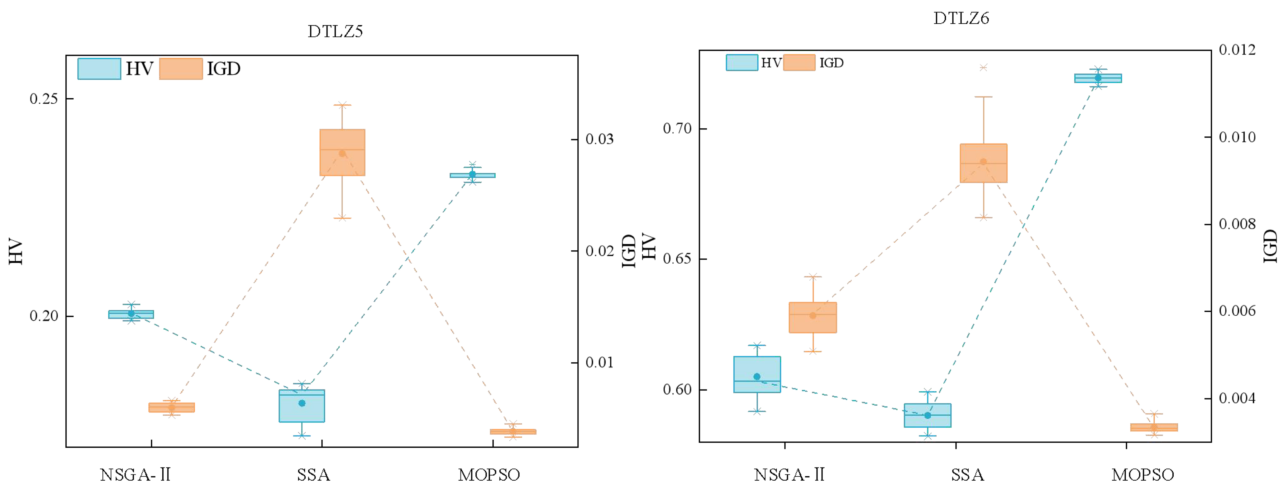
Figure 14. HV and IGD box plots. HV: Hypervolume; IGD: inverted generational distance.
Process parameter decision and verification
According to the LIME and PDP analyses above, increasing welding speed can reduce EC, but TS and IW will decrease. Conversely, increasing defocusing distance or laser power can improve TS and IW, but EC will also increase, meaning all three objectives cannot be optimized simultaneously. To balance these objectives while considering the high cost of laser welding tests, eight parameter sets from the Pareto solution interval were selected for final optimization and validation. The test results are shown in Figure 15. The optimized parameters reduced average EC by 28.98%, increased average TS by 25.93%, and increased the average IW by 13.08%. Overall, the improvements in EC and TS were more pronounced than those of IW.
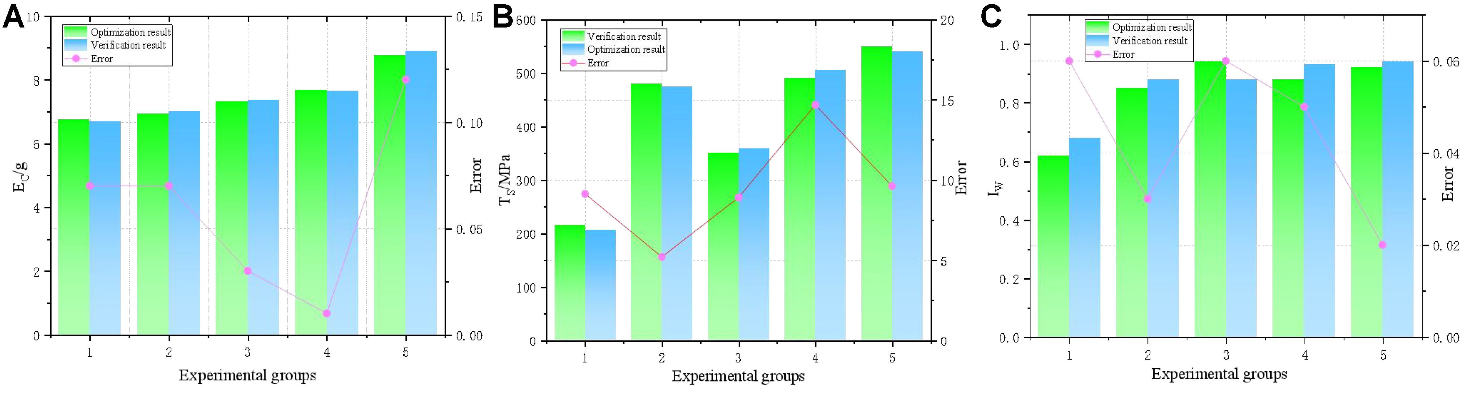
Figure 15. Validation of optimization results for (A) EC; (B) IW; and (C) TS. EC: Carbon emissions; IW: weld depth-to-width ratio; TS: tensile strength.
CONCLUSIONS
This work presents a hybrid optimization framework that integrates stacked machine learning models with a MOPSO strategy to jointly address weld quality and environmental impact. The proposed approach not only demonstrated superior predictive accuracy and robustness compared with conventional single models, but also yielded optimized process parameters that simultaneously reduced EC and enhanced tensile properties as well as bead morphology. These results confirm the feasibility of coupling data-driven modeling with advanced optimization techniques to achieve greener and more reliable laser welding of 316L stainless steel. Moreover, the framework highlights a pathway for embedding sustainability considerations into manufacturing process design, offering insights for broader industrial adoption.
Beyond the technical results, this work highlights the sustainability potential of advanced process parameter optimization. By explicitly linking welding parameters to both energy efficiency and emission reduction, the study provides insights into greener manufacturing practices. Such improvements are particularly valuable for industries with high energy demand, where optimizing welding processes can contribute to broader carbon reduction goals and align with global initiatives in sustainable manufacturing.
Nevertheless, the research is not without limitations. The scope of parameters considered was restricted to laser power, welding speed, and defocusing distance, while other influential factors such as shielding gas composition or beam oscillation were not included. Additionally, the dataset, though carefully designed, remains modest in scale, which may affect the generalizability of the predictive model under more diverse conditions.
Future research will address these limitations by expanding experimental and simulated datasets, incorporating additional process parameters, and developing adaptive control strategies for real-time optimization. Moreover, translating the proposed framework into industrial digital twin systems and welding process databases could accelerate its adoption in large-scale production. Such integration would not only support process-level optimization but also foster industry-wide efforts toward sustainable, low-carbon, and high-quality manufacturing.
DECLARATIONS
Authors’ contributions
Made substantial contributions to conception and design of the study and performed data analysis and interpretation: Li, S.; Wu, J.
Performed data acquisition and provided administrative, technical, and material support: Li, C.; Zhang, C.; Xie, Y.
Availability of data and materials
The data supporting the findings of this study are available from the corresponding author upon reasonable request.
Financial support and sponsorship
This work was supported by the National Natural Science Foundation of China (Grant No. 52205527), the National Natural Science Foundation of China (Grant No. 52075229), and the Natural Science Foundation of Jiangsu (Grant No. 22KJB460018).
Conflicts of interest
Wu, J. is a Guest Editor of Journal of Materials Informatics, but was not involved in any steps of the editorial process, notably including reviewer selection, manuscript handling, or decision-making, while the other authors have declared that they have no conflicts of interest.
Ethical approval and consent to participate
Not applicable.
Consent for publication
Not applicable.
Copyright
© The Author(s) 2026.
REFERENCES
1. Song, L.; Wang, C.; Li, Y.; Wei, X. Predicting stacking fault energy in austenitic stainless steels via physical metallurgy-based machine learning approaches. J. Mater. Inf. 2025, 5, 2.
2. Su, G.; Xie, D.; Wu, F.; et al. Corrosion mechanisms of 316L stainless steel in polyphosphoric acid at elevated temperature: behavior and mechanistic insights. Corros. Sci. 2024, 236, 112277.
3. Ge, W.; Cao, H.; Li, H.; Zhang, C.; Li, C.; Wen, X. Multi-feature driven carbon emission time series coupling model for laser welding system. J. Manuf. Syst. 2022, 65, 767-84.
4. You, D.; Li, Y.; Li, F.; et al. Effect of laser shock peening on the fatigue performance of Q355D steel butt-welded joints. J. Manuf. Mater. Process. 2025, 9, 273.
5. Wei, H.; Zhang, Y.; Tan, L.; Zhong, Z. Energy efficiency evaluation of hot-wire laser welding based on process characteristic and power consumption. J. Clean. Prod. 2015, 87, 255-62.
6. Le-Quang, T.; Faivre, N.; Vakili-Farahani, F.; Wasmer, K. Energy-efficient laser welding with beam oscillating technique - a parametric study. J. Clean. Prod. 2021, 313, 127796.
7. Yilbas, B. S.; Shaukat, M. M.; Afzal, A. A.; Ashraf, F. Life cycle analysis for laser welding of alloys. Opt. Laser. Technol. 2020, 126, 106064.
8. Jiang, P.; Wang, C.; Zhou, Q.; Shao, X.; Shu, L.; Li, X. Optimization of laser welding process parameters of stainless steel 316L using FEM, Kriging and NSGA-II. Adv. Eng. Softw. 2016, 99, 147-60.
9. Yang, Y.; Cao, L.; Zhou, Q.; Wang, C.; Wu, Q.; Jiang, P. Multi-objective process parameters optimization of laser-magnetic hybrid welding combining Kriging and NSGA-II. Robot. Comput. Integr. Manuf. 2018, 49, 253-62.
10. IEA. CO2 Emissions in 2022. https://www.iea.org/reports/co2-emissions-in-2022. (accessed 23 Jan 2026).
11. Ghari, H.; Taherizadeh, A.; Sadeghian, B.; Sadeghi, B.; Cavaliere, P. Metallurgical characteristics of aluminum-steel joints manufactured by rotary friction welding: a review and statistical analysis. J. Mater. Res. Technol. 2024, 30, 2520-50.
12. Winiczenko, R.; Skibicki, A.; Skoczylas, P. Multi-objective optimisation of welding parameters for AZ91D/AA6082 rotary friction welded joints. Appl. Sci. 2025, 15, 1477.
13. Kahhal, P.; Ghasemi, M.; Kashfi, M.; Ghorbani-Menghari, H.; Kim, J. H. A multi-objective optimization using response surface model coupled with particle swarm algorithm on FSW process parameters. Sci. Rep. 2022, 12, 2837.
14. Li, C.; Tang, Y.; Cui, L.; Li, P. A quantitative approach to analyze carbon emissions of CNC-based machining systems. J. Intell. Manuf. 2015, 26, 911-22.
15. Peng, G.; Ma, L.; Hong, S.; Ji, G.; Chang, H. Optimization design and internal flow characteristics analysis based on latin hypercube sampling method. Arab. J. Sci. Eng. 2025, 50, 2715-54.
16. Mou, X.; Huang, X.; Ma, G.; et al. Prediction of Storage quality and multi-objective optimization of storage conditions for fresh Lycium barbarum L. based on optimized latin hypercube sampling. Foods 2025, 14, 2807.
17. Park, J.; Ryu, I.; Ryu, D.; Lee, Y. An efficient near-optimal Latin hypercube design for large datasets. J. Mech. Sci. Technol. 2025, 39, 315-28.
18. Ma, J.; Xia, D.; Guo, H.; et al. Metaheuristic-based support vector regression for landslide displacement prediction: a comparative study. Landslides 2022, 19, 2489-511.
19. Imani, M.; Beikmohammadi, A.; Arabnia, H. R. Comprehensive analysis of random forest and XGBoost performance with SMOTE, ADASYN, and GNUS under varying imbalance levels. Technologies 2025, 13, 88.
20. Niazkar, M.; Menapace, A.; Brentan, B.; et al. Applications of XGBoost in water resources engineering: a systematic literature review (Dec 2018 - May 2023). Environ. Model. Softw. 2024, 174, 105971.
21. Li, X.; Shi, L.; Shi, Y.; et al. Exploring interactive and nonlinear effects of key factors on intercity travel mode choice using XGBoost. Appl. Geogr. 2024, 166, 103264.
22. Erdogan Erten, G.; Yavuz, M.; Deutsch, C. V. Combination of machine learning and Kriging for spatial estimation of geological attributes. Nat. Resour. Res. 2022, 31, 191-213.
23. Takoutsing, B.; Heuvelink, G. B. Comparing the prediction performance, uncertainty quantification and extrapolation potential of regression Kriging and random forest while accounting for soil measurement errors. Geoderma 2022, 428, 116192.
24. Bahrami, B.; Khayyambashi, M. R.; Mirjalili, S. Multiobjective placement of edge servers in MEC environment using a hybrid algorithm based on NSGA-II and MOPSO. IEEE. Internet. Things. J. 2024, 11, 29819-37.
25. Nagayo, A. M.; Singh, R.; Dhawan, A.; et al. Integrating environmental sustainability in construction time-cost trade-off for decision-making using hybrid NSGA-III and MOPSO approach. Asian. J. Civ. Eng. 2025, 26, 1527-42.
26. Agarwal, A. K.; Chauhan, S. S.; Sharma, K.; Sethi, K. C. Development of time–cost trade-off optimization model for construction projects with MOPSO technique. Asian. J. Civ. Eng. 2024, 25, 4529-39.
27. Chowdhury, S.; Bohre, A. K.; Saha, A. K. Meta-Heuristic optimization for hybrid renewable energy system in Durgapur: performance comparison of GWO, TLBO, and MOPSO. Sustainability 2025, 17, 6954.
28. Kim, H. Y. Analysis of variance (ANOVA) comparing means of more than two groups. Restor. Dent. Endod. 2014, 39, 74-7.
29. Chen, W.; Carrera Uribe, M.; Kwon, E. E.; et al. A comprehensive review of thermoelectric generation optimization by statistical approach: Taguchi method, analysis of variance (ANOVA), and response surface methodology (RSM). Renew. Sustain. Energy. Rev. 2022, 169, 112917.
30. Guo, Q.; Liu, Y.; Chen, B.; Yao, Q. A variable and mode sensitivity analysis method for structural system using a novel active learning Kriging model. Reliab. Eng. Syst. Saf. 2021, 206, 107285.
31. Xiao, N.; Yuan, K.; Zhou, C. Adaptive Kriging-based efficient reliability method for structural systems with multiple failure modes and mixed variables. Comput. Methods. Appl. Mech. Eng. 2020, 359, 112649.
32. Vimbi, V.; Shaffi, N.; Mahmud, M. Interpreting artificial intelligence models: a systematic review on the application of LIME and SHAP in Alzheimer’s disease detection. Brain. Inform. 2024, 11, 10.
Cite This Article
How to Cite
Download Citation
Export Citation File:
Type of Import
Tips on Downloading Citation
Citation Manager File Format
Type of Import
Direct Import: When the Direct Import option is selected (the default state), a dialogue box will give you the option to Save or Open the downloaded citation data. Choosing Open will either launch your citation manager or give you a choice of applications with which to use the metadata. The Save option saves the file locally for later use.
Indirect Import: When the Indirect Import option is selected, the metadata is displayed and may be copied and pasted as needed.
About This Article
Special Topic
Copyright

Data & Comments
Data
0


Comments
Comments must be written in English. Spam, offensive content, impersonation, and private information will not be permitted. If any comment is reported and identified as inappropriate content by OAE staff, the comment will be removed without notice. If you have any queries or need any help, please contact us at [email protected].