

AD-FIT: industrial anomaly detection via fusion of IoT sensing and network traffic data
 0
0 Graphical Abstract
Abstract
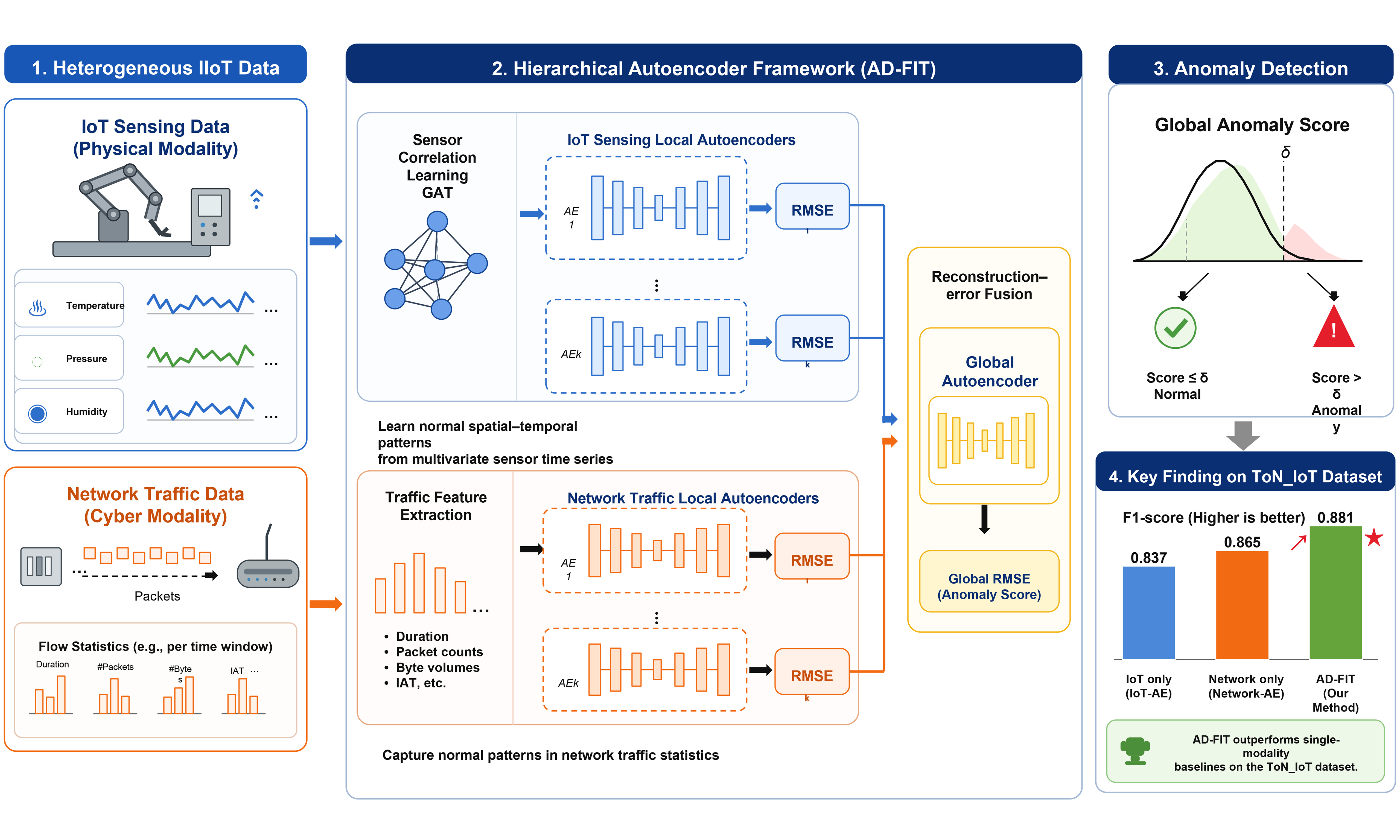
Anomaly detection is an important research topic in the Industrial Internet of Things (IIoT). In recent years, deep learning has been exploited to analyze complex IIoT data and build anomaly detection models. Due to the lack of abnormal samples and the difficulty of labeling industrial data, unsupervised deep learning has become the mainstream technique for IIoT anomaly detection, with autoencoders being the most representative approaches. However, the existing autoencoder-based IIoT anomaly detection models predominantly focus on a single data modality, since existing data fusion frameworks are mostly designed for supervised learning tasks, while it is infeasible to simultaneously reconstruct heterogeneous data modalities in a unified autoencoder. To address this limitation, this paper focuses on IoT sensing data and network traffic data and proposes AD-FIT, a novel autoencoder framework for IIoT anomaly detection via the fusion of IoT sensing and network traffic data in an unsupervised manner. Specifically, it creates multiple local autoencoders with different architectures to fit the two data modalities, and then fuses their reconstruction errors through a global autoencoder. We conducted extensive experiments based on a public IIoT dataset. Experimental results show that AD-FIT achieves the best overall anomaly detection performance among the evaluated baseline methods, with F1-score improvements ranging from 7.1% to 38.6%.
Keywords


 Download PDF
1. INTRODUCTION
In recent years, the advent of the Industrial Internet of Things (IIoT) has transformed traditional industrial landscapes by integrating advanced connectivity and smart technologies into manufacturing processes. IIoT systems encompass a myriad of interconnected devices and sensors that collectively contribute to the efficient monitoring and control of industrial operations. This paradigm shift has not only ushered in a new era of productivity but has also introduced novel challenges, particularly in the realm of anomaly detection, which is the identification of deviations from expected behavior. An anomaly can indicate a malfunction, an attack, or other types of unexpected events[1]. Early detection of anomalies can prevent equipment failures, improve process efficiency, and enhance overall performance.
To facilitate information exchange among humans, devices, and systems, an IIoT system connects a large number of monitoring devices and sensors through communication networks and collects data that can reflect the process and status of production. As a result, most state-of-the-art IIoT anomaly detection methods apply data-driven techniques, including traditional machine learning and deep learning. Since the operating processes and collected IIoT data are highly complex, making it difficult to understand the abnormal states, labeling anomalous states in the collected IIoT data requires substantial domain knowledge and is costly. In practice, obtaining labeled abnormal samples from real IIoT systems is often difficult or impossible. Therefore, most previous studies focus on unsupervised learning techniques[2,3]. Studies using traditional machine learning typically involve two steps. They first extract a large number of features from industrial data, and then discover anomalies by using outlier detection algorithms [e.g., clustering[4,5], One-Class support vector machine (SVM)[6], iForest[7]]. However, feature engineering relies on domain knowledge, and the high-dimensional and dynamic nature of IIoT data makes it difficult to design effective features.
In recent years, thanks to the ability to automatically learn features from raw data, deep learning has been increasingly applied to IIoT anomaly detection tasks. Many studies focus on multivariate time-series IoT sensing data and use unsupervised reconstruction-based deep learning models[8,9]. These models learn representations of normal patterns and detect anomalies using reconstruction errors. Due to the temporal nature of IoT sensing data, recurrent neural network (RNN)-based models have also been widely investigated[8,10]. Several studies have also attempted to detect anomalies from the IIoT network traffic data. Specifically, they extract statistical and temporal features from raw network data packets[11] and build anomaly detection models based on autoencoders[12,13]. Various backbone networks [e.g., multilayer perceptron (MLP)[13], long short-term memory (LSTM)[14]] that can adapt to these statistical and temporal features are exploited to implement the autoencoders. Then, these features are reconstructed based on the decoders, and the reconstruction errors are used for network traffic anomaly detection. Recent work has further applied sequence-to-sequence LSTM autoencoders with attention mechanisms to real-time network-based anomaly detection in Modbus/TCP industrial control systems[15].
Recent transformer and graph-based methods, including Anomaly Transformer, TranAD, GRELEN, MTGFlow, MEMTO, D3R, SARAD, and graph mixture-of-experts models, further improve multivariate time-series anomaly detection by modeling temporal dependencies, inter-variable relations, and nonstationary behavior[16-23]. Multimodal sensing representation learning, as exemplified by FOCAL, also shows the value of contrastive alignment across heterogeneous sensing signals[24]. Recent IIoT intrusion-detection research also benefits from realistic benchmarks and attention-based models, including Edge-IIoTset, CICIoT2023, and SACNN-IDS[25-27].
Despite recent advances, existing IIoT anomaly-detection studies mainly focus on a single data modality and stable operating conditions. Although dynamic weighted domain adaptation has been explored for bearing fault diagnosis under time-varying speeds[28], robust unsupervised fusion of heterogeneous IoT sensing and network traffic data remains insufficiently explored, limiting the ability to detect anomalies spanning both domains. Modern IIoT systems are highly interconnected, and anomalies arising in one domain may affect the entire infrastructure. Therefore, a unified framework that can effectively integrate information from both data sources is needed. However, developing such a framework remains challenging for the following reasons.
Complex correlations: IoT sensing data are usually collected from many sensors, and network traffic data are usually represented by many features, resulting in high-dimensional data. Different dimensions may have mutual correlations. For example, the data of one sensor could affect the data of another sensor, and a specific state of the system can be jointly influenced by multiple features. Moreover, the IoT sensing and network traffic data have substantially different correlation patterns, which are difficult to learn with a single unified model.
Heterogeneous data modalities: The IoT sensing data and network traffic data represent fundamentally distinct forms of information. The inherent differences in structure, format, and semantics make it challenging to seamlessly map these diverse data types into a unified feature space. Although previous work has extensively studied heterogeneous data fusion methods, most are designed for supervised learning tasks, and it is infeasible to simultaneously reconstruct heterogeneous data modalities in a unified autoencoder.
To this end, we propose AD-FIT, a novel framework for IIoT anomaly detection that fuses IoT sensing and network traffic data. AD-FIT adopts the following strategies to address the above-mentioned challenges. First, AD-FIT uses graphs to explicitly model the correlations between different feature dimensions and applies graph neural networks (GNNs) to learn the correlation strengths and incorporate them into the anomaly detection model. Second, AD-FIT fuses the IoT sensing data and network traffic data based on an ensemble framework of autoencoders across diverse data modalities. In summary, this paper makes the following contributions.
First, we propose an ensemble framework to fuse multiple autoencoders across two data modalities, i.e., IoT sensing data and network traffic data. This framework operates unsupervisedly and does not require anomalous training samples.
Second, we design the autoencoders using GNNs to explicitly learn complex correlations between sensors and integrate them into the models.
Third, we conducted extensive experiments on a public multimodal IIoT dataset. The results show that AD-FIT improves the F1-score by approximately 7.1% to 38.6% compared with the baseline methods.
2. RELATED WORK
2.1. Industrial anomaly detection
Industrial data are typically multivariate time series characterized by large volume, high dimensionality, and strong temporal dynamics, and thus the traditional univariate anomaly detection methods[2-6] may not perform effectively.
To handle complex multivariate time-series data, most existing studies use learning-based techniques (including machine learning and deep learning), which can be roughly divided into two categories, i.e., supervised learning techniques and unsupervised learning techniques. In terms of supervised learning techniques, Griffin et al. proposed an anomaly detection method based on neural networks and decision trees to detect anomalies across multiple industrial processes[29]. Nanduri et al. proposed the use of recurrent neural networks to detect abnormal events that may reduce flight safety factors[10]. Janssens et al. proposed a convolutional neural network (CNN)-based feature-learning system for detecting fault states in rotating machinery[30].
Although supervised learning techniques can better distinguish anomalies by explicitly learning the latent patterns from anomaly samples, their practical deployment is challenging because labeled anomalous training data are severely limited. Because normal industrial data can be easily obtained at scale, unsupervised learning techniques are widely used for industrial multivariate time-series anomaly detection. Earlier studies applied traditional unsupervised machine-learning methods such as clustering, One-Class SVM, and iForest. For example, Amruthnath and Gupta applied multiple clustering algorithms for anomaly detection (e.g., K-Means, fuzzy C-Means)[31]. These algorithms identify behaviors that deviate from normal patterns. Diez-Olivan et al. proposed an anomaly detection method based on One-Class SVM to detect anomalies in sensor data by obtaining anomaly scores based on the distance between samples and the separating hyperplane[32]. Joshi et al. conducted anomaly detection based on a hidden Markov model (HMM), which constructs a model by extracting features and estimating anomaly probabilities from the generated state sequence[33]. Nguyen and Vien proposed AE-1SVM, which combines autoencoder-based representation learning with a One-Class SVM for unsupervised anomaly detection[34].
However, traditional machine-learning techniques rely heavily on feature engineering, which is challenging for high-dimensional and dynamic industrial data. Consequently, researchers have extensively investigated generative encoder-decoder networks for unsupervised anomaly detection in time-series data. For example, Xu et al. proposed Donut, a variational autoencoder (VAE)-based unsupervised anomaly detection method that identifies abnormal time points using the reconstruction probability of time-series observations[35]. Lu et al. detected anomalies in rotating mechanical components by using a stacked autoencoder[36]. Zhang et al. proposed MSCRED, which uses a ConvLSTM autoencoder to learn the multiple levels of system operation patterns characterized by multi-scale signature matrices in different time steps[37]. Yin et al. integrated a CNN with a recurrent autoencoder for detecting anomalies in IoT systems[38]. Specifically, they used a two-stage sliding window strategy to design the encoder for better feature extraction. Muneer et al. proposed a hybrid model based on a deep autoencoder neural network (DANN) with five layers for detecting anomalies in a real-world gas turbine dataset[39]. Although the encoder-decoder deep neural networks have achieved promising results for industrial anomaly detection, their performance may be further improved by explicitly learning the relationships between industrial data and network traffic data and appropriately balancing the two data sources.
2.2. Cross-domain data fusion
IoT sensing data and network traffic data represent distinct modalities with different representations, distributions, scales, and densities. For example, industrial sensing data typically consist of measurements collected by multiple sensor devices on a production line, which may include data such as device temperature and pressure. Network traffic data, by contrast, come from packet analysis and include attributes such as source and destination addresses. Consequently, fusing data across these modalities is challenging. Data fusion methods can be categorized as stage-based fusion methods, feature-level fusion methods, and semantic-level fusion methods[40].
The stage-based methods use different datasets at different stages of a data fusion task. Thus, these datasets are loosely connected, and cross-modal consistency is not explicitly required. For example, Xiao et al. utilized spatial trajectories to detect stay points, converting them into feature vectors based on surrounding points of interest (POIs)[41]. These feature vectors are hierarchically clustered to form a tree structure, representing users’ location histories and facilitating similarity measurement between users based on their hierarchical graphs.
For feature-level fusion, a common approach is to learn a unified feature representation from disparate datasets using deep neural networks. For example, Ngiam et al. introduced a deep autoencoder architecture to capture intermediate feature representations across modalities, exploring three learning settings: cross-modality learning, shared representation learning, and multimodal fusion, thereby improving single-modality representations and capturing correlations across multiple modalities[42]. Nagrani et al. introduced a transformer-based multimodal architecture that uses attention bottlenecks to constrain cross-modal interactions through a small set of bottleneck latent units, thereby improving fusion performance while reducing computational cost[43]. More recently, IoT-GRAF represents heterogeneous sensing and network observations through graph learning for multimodal IoT anomaly and intrusion detection[44]. Cross-domain representation learning has also been used to jointly capture network behaviors and physical-process states in industrial control systems[45].
Feature-based data fusion methods treat features as numerical or categorical values without considering their semantic meaning, whereas semantic-level methods capture the semantic information contained in each dataset, recognize relations between features, and provide interpretable and meaningful fusion by incorporating the significance of each dataset and the interplay among the datasets. Although researchers have investigated cross-domain fusion methods, their scope is often limited to specific data-query or application settings. For example, Sun et al. studied k-nearest-neighbor temporal aggregate queries that rank locations by combining spatial distance with temporally aggregated attributes[46]. Decision-level fusion of network and physical anomaly detectors has been shown to improve cyber–physical threat detection compared with relying on either data source alone[47]. More recently, an unsupervised adversarial fusion framework combined sensor and network representations through dual cross-attention to detect subtle cyber–physical anomalies[48]. Despite this progress, robust unsupervised fusion of heterogeneous sensing and network-traffic modalities for IIoT anomaly detection remains insufficiently explored.
3. METHODOLOGY
3.1. Preliminary
In this section, we first define the key concepts and formulate the anomaly detection problem. We then introduce the overall AD-FIT architecture, followed by the modality-specific backbone autoencoders, the unsupervised data-fusion framework, and the final anomaly-detection procedure.
Definition 1 (IoT Sensing Sample): The IoT sensing sample of time slot t is denoted as Xt ∈ RN×W, where N is the number of sensors, and W is the sampling-window length. Here, Xt is a subsequence of the multivariate time series from the N sensors during the time period of (t-W, t]. Note that a physical sensor may generate multiple readings at each time slot, e.g., an accelerometer generates three readings at each time slot. For notational convenience, we treat each univariate time series in Xt as sampled from an individual virtual sensor.
Definition 2 (Network Traffic Sample): The network traffic sample of time slot t (denoted as Yt) is the collection of network data packets captured during the time period of (t-W, t].
Definition 3 (IIoT Data Sample): The IIoT data sample of time slot t, denoted as St = (Xt, Yt), is composed of an IoT sensing sample and a network traffic sample during the same time period (t-W, t].
Problem Definition: Industrial anomaly detection in this paper is formulated as learning from IIoT data samples to obtain a function f, which takes St as input and produces an output value yt ∈ {0, 1}, where yt denotes whether an anomaly occurs at time slot t.
Architecture of AD-FIT: Figure 1 shows the architecture of AD-FIT, which comprises three modules, i.e., IoT-AE module, Network-AE module, and Fusion module. The IoT-AE module applies bootstrap sampling to the IoT sensing samples to create multiple training subsets and then trains multiple autoencoders on the IoT sensing data. Each IoT sensing autoencoder consists of three layers: the graph attention network (GAT) layer, the encoder layer, and the decoder layer. The Network-AE module also applies bootstrap sampling to the set of network traffic samples to create multiple training subsets and then trains multiple autoencoders on the network traffic data. Each autoencoder for network traffic data consists of three layers, i.e., the feature extraction layer, the encoder layer, and the decoder layer. The Fusion module can be viewed as a meta-learner on top of the IoT-AE and Network-AE modules. It takes the reconstruction root mean square errors (RMSEs) produced by the local autoencoders as input and trains a global autoencoder to reconstruct these RMSEs.
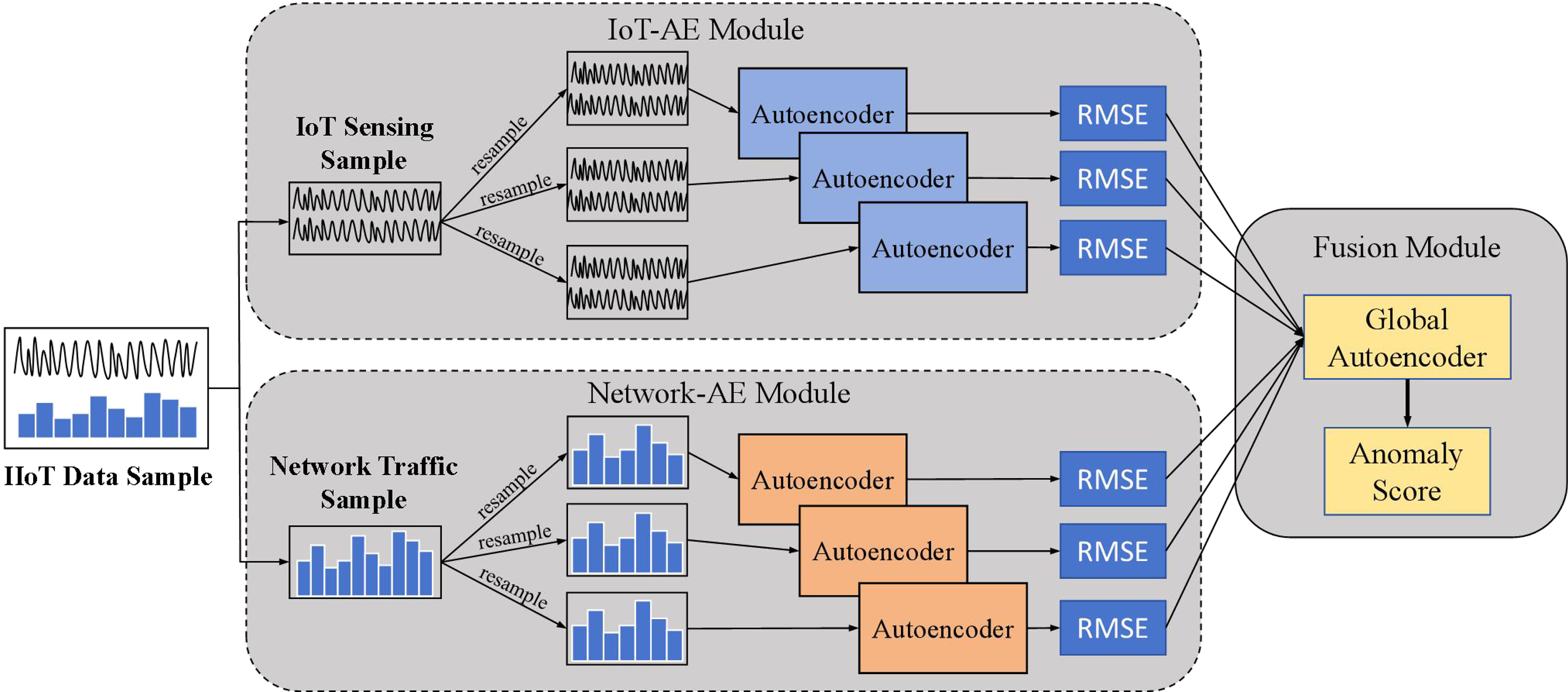
Figure 1. The architecture of AD-FIT. IIoT: Industrial Internet of Things; IoT: Internet of Things; AE: autoencoder; RMSE: root mean square error.
In the real-time anomaly detection phase, given an IIoT data sample St = (Xt, Yt), Xt and Yt are fed into the corresponding autoencoders of the IoT-AE and Network-AE modules, respectively, which produce a series of reconstruction RMSEs. The Fusion module then combines these RMSEs to produce a global RMSE for anomaly detection.
AD-FIT assumes that the input IoT sensing and network-traffic data have undergone basic quality control and are sufficiently reliable. In practical IIoT deployments, sensor drift, missing measurements, and corrupted readings may distort reconstruction errors and propagate to the fusion decision. Although the present framework does not explicitly model reliability and trust, reliability-aware data validation or weighting could be incorporated to improve deployment robustness[49].
3.2. The backbone autoencoders
AD-FIT is essentially an ensemble framework of autoencoders, built separately for IoT sensing data and network traffic data before fusion. Because the two data modalities have different characteristics, we used different backbone autoencoders for each.
3.2.1. IoT sensing data-based autoencoder
The backbone autoencoder for IoT sensing data is composed of three layers, i.e., the GAT layer, the encoder layer, and the decoder layer. The GAT layer learns potential correlations between different sensors. The encoder layer learns spatial and temporal patterns in IoT sensing data. The decoder layer reconstructs the input data.
(1) The GAT Layer
The IoT sensing data are represented as high-dimensional multivariate time series. First, these dimensions, which represent different sensors, may exhibit potential correlations and cross-effects. For example, detecting some anomalies requires considering data from multiple sensors simultaneously. Second, different sensors may contribute differently to anomaly detection. For example, pressure data in a hydraulic system are usually more important for anomaly detection than the data from other sensors. To address these issues, the GAT layer uses a graph to model the correlations between different dimensions of the IoT sensing data (Step 1), and then the correlation strengths are learned using a GAT subnetwork (Step 2).
Step 1 (Sensor graph construction): A sensor graph is represented as G = (V, E, F), where each node vi ∈ V represents a dimension of the IoT sensing data (corresponding to a sensor), each edge eij ∈ E represents a correlation between sensor vi and vj, and F represents the set of node features, where each element fi denotes the original feature of node vi (i.e., the univariate time-series data collected from sensor vi). Domain knowledge can determine whether two sensors are correlated when constructing the sensor graph. However, because domain knowledge is often hard to obtain, we design G as a fully connected graph when domain knowledge is unavailable.
Step 2 (Correlation strength learning): Following the graph attention mechanism proposed by Veličković et al.[50], we apply GAT to learn the correlation strength between each pair of nodes in G. As illustrated in Figure 2, for each edge eij in G, its correlation strength wij is calculated according to Equation (1), where aij is the unnormalized attention score, k is the index of a node in the first-order neighborhood of vi, and L is the number of nodes in this neighborhood, including vi itself.
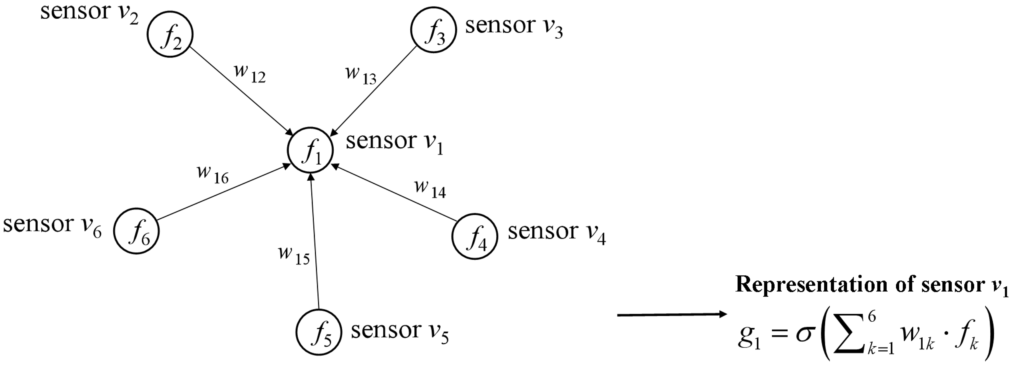
Figure 2. Correlation-strength learning based on GAT. GAT: Graph attention network.
The unnormalized attention score aij is further calculated according to Equation (2), where q is a learnable parameter vector and σ(…) is a nonlinear activation function.
The normalized correlation strengths are subsequently used to aggregate the neighboring features and update the embedding gi of node vi according to Equation (3), where wik is the normalized correlation strength from node vk to node vi and fk is the original feature of node vk.
After the two steps, each IoT sensing sample Xt is represented as a feature matrix GXt ∈ RN×W, where the i-th row of GXt represents the embedding vector of node vi (i.e., gi).
(2) The Encoder Layer
The autoencoder maps the original IoT sensing samples into a lower-dimensional latent feature space using an encoder and then reconstructs the latent features into the original sample space using a decoder. The autoencoder was trained by gradually reducing the errors between original samples and reconstructed samples through backpropagation.
Because the latent features have lower dimensionality than the original samples, the latent features can capture the dominant patterns of the original samples. For the anomaly detection task, the autoencoder is trained based on normal samples (or mostly normal samples), so the latent features learned by the trained autoencoder can represent the dominant patterns of normal samples. If a reconstructed sample deviates greatly from the original, it means the original sample does not conform to the main patterns of normal samples, indicating an anomaly.
Considering the temporal characteristics of IoT sensing samples, we employ an LSTM encoder based on the recurrent architecture proposed by Hochreiter and Schmidhuber[51]. As shown in Figure 3, given an IoT sensing sample Xt = [xt-W+1, xt-W+2, …, xt] (xt ∈ RN×1 denotes the sensor-reading vector at time slot t), we first input Xt into the GAT layer to obtain the updated feature matrix GXt = [gxt-W+1, gxt-W+2, …, gxt]. At each time slot t, the encoder updates its hidden state htie from the previous state ht-1ie and the current GAT-enhanced feature gxt according to Equation (4), where the superscript “ie” denotes the IoT sensing data encoder.
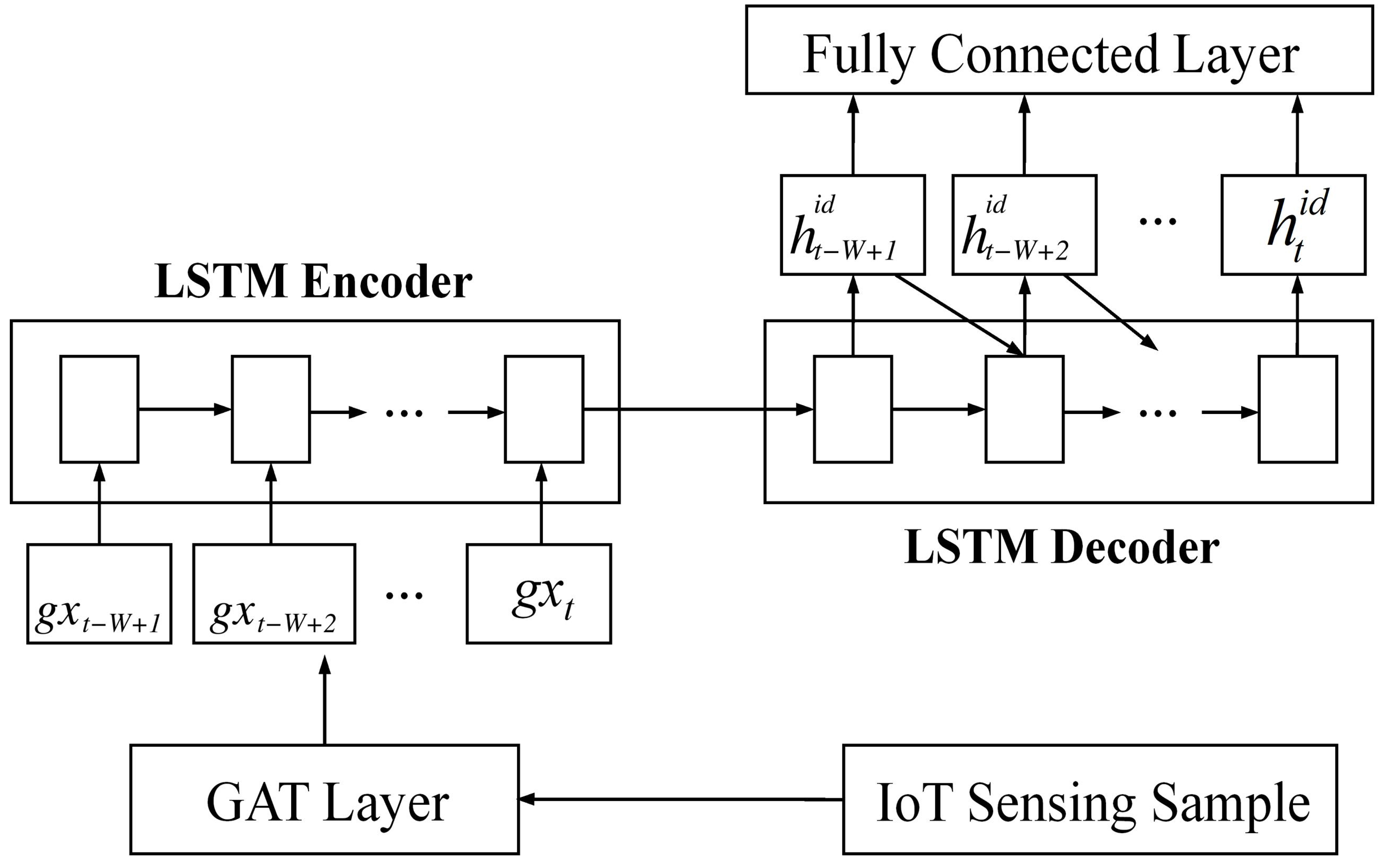
Figure 3. The architecture of the LSTM autoencoder. LSTM: Long short-term memory; GAT: graph attention network; IoT: Internet of Things.
(3) The Decoder Layer
As shown in Figure 3, the decoder takes htie as input and also uses an LSTM subnetwork to output W hidden state vectors ht-W+1id, ht-W+2id, …, htid based on Equation (5). After that, a fully connected subnetwork is used to reconstruct ht-W+1id, ht-W+2id, …, htid into the same dimensions as the original samples
Following the reconstruction-error objective commonly used in LSTM-based autoencoders, we train the autoencoder for IoT sensing data by minimizing the RMSE between the original sample Xt and its reconstruction
3.2.2. Network traffic data-based autoencoder
The backbone autoencoder for network traffic data is composed of three layers, i.e., the feature extraction layer, the encoder layer, and the decoder layer.
(1) The Feature Extraction Layer
The feature extraction layer includes two steps, i.e., sample generation and feature extraction.
Sample generation: The network data packets can be captured using tools such as tcpdump and Wireshark. Then, we generate network traffic samples by selecting network data packets for a specific source-destination pair (same source IP, destination IP, source port, destination port, and protocol) within a specific time period (t-W, t].
Feature extraction: We used CICFlowMeter (https://github.com/ahlashkari/CICFlowMeter) to extract a fixed set of statistical features from each network-traffic sample. These features characterize flow duration, packet counts and byte volumes in the forward and backward directions, packet-length statistics, transmission rates, and packet inter-arrival times. Identifier fields and label-related fields are excluded. The remaining numerical features are normalized using statistics calculated from the training set and are assembled into an M-dimensional vector yt ∈ RM×1.
(2) The Encoder Layer
We used an MLP as the encoder for the network traffic samples. Given a network traffic sample yt, the encoder layer maps yt to a latent feature space. Specifically, a two-layer MLP is applied, as shown in Equation (7), where W(i) and b(i) denote the learnable weight matrix and bias vector of the i-th hidden layer, respectively.
(3) The Decoder Layer
The decoder layer’s task is to reconstruct the latent feature hne(2) back to the input space. We also apply a two-layer MLP as the decoder, which outputs a reconstructed sample
3.3. Data fusion via ensemble of autoencoders
3.3.1. Unsupervised data fusion framework
Because IoT sensing data and network traffic data typically have distinct dimensions and characteristics, a single, unified autoencoder cannot process both. Instead, we used autoencoders with different structures to model them. However, IoT sensing data and network traffic data collected from the same IIoT system may exhibit semantic correlations. For example, in a smart home environment, an attacker could remotely control a door lock. Because attack behaviors involve infiltrating the household’s smart home network and lurking on edge devices, clues can be reflected in both network traffic data and device log data. Therefore, a data fusion mechanism is needed to learn semantic correlations across the IoT sensing data and network traffic data.
However, existing data fusion frameworks are designed for supervised learning tasks. For example, the most popular traditional data fusion frameworks (including Bagging[52], Boosting[53], and Stacking[54]) perform data fusion by exploiting classification consistency, classification residual, or classification probability distribution, whereas such information is unavailable in unsupervised settings. Deep learning models usually perform data fusion by integrating different subnetworks in a unified learning objective. Unfortunately, it is infeasible to simultaneously reconstruct heterogeneous data modalities in a unified autoencoder.
To address this challenge, we propose a data-fusion framework for autoencoders with different data modalities. As shown in Figure 4, this framework comprises three parts: data sampling, local autoencoder training, and global autoencoder training.
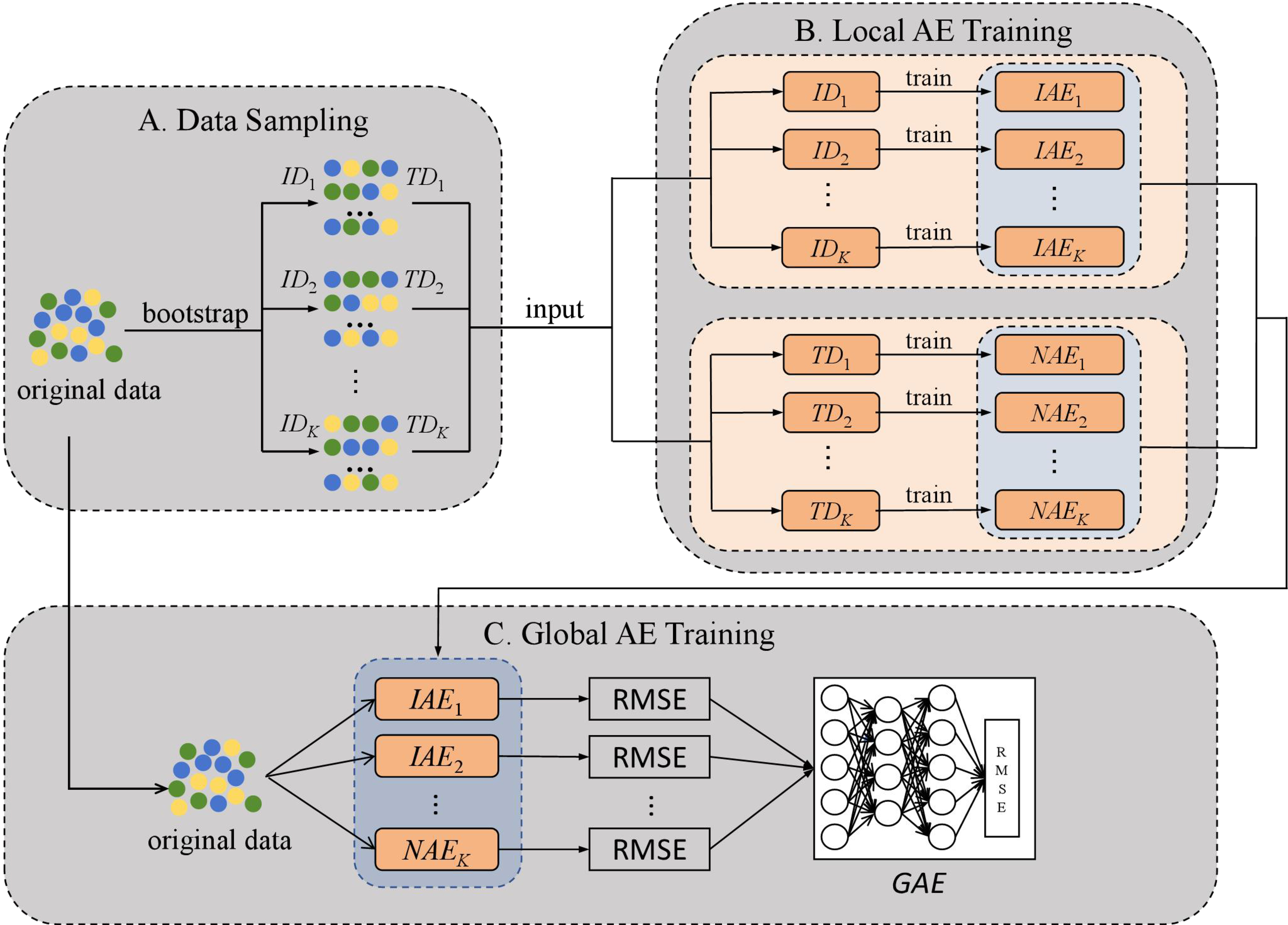
Figure 4. The data fusion framework for autoencoders. AE: Autoencoder; RMSE: root mean square error; GAE: global autoencoder.
(1) Data Sampling
Ensembling multiple sub-models is an effective approach for data fusion. Diversity among component models is an important factor affecting ensemble performance[55]. Thus, we used bootstrap sampling to create multiple training subsets for both IoT sensing data and network traffic data. Specifically, given a training dataset D, we perform K bootstrap iterations. In each iteration, a training subset is generated by randomly selecting NS samples from D with replacement, which means that a sample in D can be selected multiple times or not at all in the training subset. By applying bootstrap sampling, we can generate diverse training subsets for each data modality.
Finally, we can obtain K training subsets for both IoT sensing data (denoted as IDS = {ID1, ID2, …, IDK}) and network traffic data (denoted as TDS = {TD1, TD2, …, TDK}).
(2) Local Autoencoder Training
After obtaining the collections of training subsets IDS and TDS for both data modalities, we train multiple autoencoders through the following steps. First, for each training subset IDk in IDS, we train a backbone autoencoder for IoT sensing data (denoted as IAEk). Second, for each training subset TDk in TDS, we train a backbone autoencoder for network traffic data (denoted as NAEk). Finally, we can obtain a set of IoT sensing data-based local autoencoders IAES = {IAE1, IAE2, …, IAEK} and a set of network traffic data-based local autoencoders NAES = {NAE1, NAE2, …, NAEK}. This ensures that each training subset is used to train a dedicated local autoencoder, and the resulting collection of local autoencoders is capable of capturing diverse patterns within the IIoT data.
(3) Global Autoencoder Training
To fuse the multiple local autoencoders from IAES and NAES, we train a global autoencoder to capture their joint semantic correlations and behavioral patterns. The core idea is inspired by stacking, i.e., the global autoencoder is trained on the outputs of the local autoencoders, but in an unsupervised manner. The specific steps are as follows.
RMSE generation: Given an IIoT data sample St = (Xt, Yt), we input the IoT sensing sample Xt into each local autoencoder in IAES. For each local autoencoder IAEk, it outputs a reconstructed sample
Global autoencoder training: The global autoencoder (denoted as GAE) is trained to capture the normal patterns of the outputs of all the local autoencoders. Specifically, GAE takes an RMSE vector ES(t) as input, and outputs a reconstructed RMSE vector E
Since GAE is trained on the outputs from all data modalities and all semantic spaces, it is expected to discover latent anomalies that are difficult to detect based on a single autoencoder or a single data modality. For example, some latent and stealthy anomalies might not necessarily cause all local autoencoders to generate high reconstruction RMSEs.
3.3.2. Anomaly detection
Given an IIoT data sample St = (Xt, Yt), we first input it to the set of local autoencoders AES = {IAE1, IAE2, …, IAEK, NAE1, NAE2, …, NAEK}, which outputs a set of RMSEs ES(t) = {IRMSE(t)1, IRMSE(t)2, …, IRMSE(t)K, NRMSE(t)1, NRMSE(t)2, …, NRMSE(t)K}. Second, we input ES(t) into the global autoencoder GAE, which outputs a reconstructed RMSE vector E
4. EXPERIMENTS
This section evaluates AD-FIT through four sets of experiments. We first introduce the dataset and evaluation strategies. We then compare AD-FIT with representative baseline methods, analyze the effect of the anomaly detection threshold, examine the contribution of different data modalities through ablation experiments, and finally present representative cases to illustrate the effectiveness of the proposed data fusion framework. The experimental results are discussed together with their underlying reasons and implications.
4.1. Experiment setup
4.1.1. Dataset
We evaluated AD-FIT based on the ToN_IoT dataset[56], which includes heterogeneous data sources collected from IoT sensors and network traffic. It was collected from a realistic and large-scale testbed network designed by the IoT Lab of UNSW Canberra Cyber. The testbed network emulates a complex and scalable IIoT environment that includes virtual machines, physical systems, hacking platforms, cloud/fog platforms, and IoT sensors. Specifically, the IoT sensor subset of ToN_IoT includes 21 data dimensions sampled from 7 sensors, and the network traffic subset comprises 46 features. ToN_IoT was collected from March 31 to April 27, 2019 (spanning nearly a month), including 167 MB of IoT sensing data and 3.16 GB of network traffic data. The IoT sensing data were sampled at 1 Hz. The complete original dataset has a normal-to-abnormal event ratio of approximately 24:1. However, after preprocessing, temporal alignment, and test-sample construction, anomalous samples account for approximately 40.7% of the test set used in our experiments.
In the experiments, the window length W was set to five sampling intervals. Since the IoT sensing data were sampled at 1 Hz, each IoT sensing sample contained five consecutive observations. Non-overlapping windows with a stride of five sampling intervals were applied to both the IoT sensing data and network traffic data, and the data falling within the same time window were paired to construct an IIoT data sample.
Unless otherwise specified, K was set to 10 in all experiments. Accordingly, 10 local autoencoders were trained for each data modality, and the RMSE vector input to the global autoencoder had a dimension of 2K.
4.1.2. Evaluation strategies
To comprehensively evaluate the anomaly detection performance, we used Accuracy, Precision, Recall, and F1-score as evaluation metrics. Accuracy alone is insufficient because a model may achieve high accuracy while failing to detect anomalous events. Hence, following the standard definitions provided by Sokolova and Lapalme[57], we used Precision, Recall, and F1-score, as shown in Equations (10)-(12), where TP is the number of abnormal samples that are accurately detected, FP is the number of normal samples that are mistakenly identified as abnormal, and FN is the number of abnormal samples that are mistakenly identified as normal.
4.2. Experiment 1: Comparison Experiment
To evaluate the comparative performance of AD-FIT, we compared it with the following seven baseline methods. All these baseline methods (a) operate in an unsupervised manner without requiring anomalous training samples; (b) consider both data modalities (i.e., the IoT sensing data and network traffic data); and (c) were configured using their best-performing parameter settings.
Threshold: It first calculates the value range for each attribute in the normal samples. Then, given an IIoT data sample, if the value of any of its attributes exceeds the corresponding normal value range, it is identified as abnormal. IoT sensing samples have attributes corresponding to different sensors, while network traffic samples have attributes that are extracted statistical features.
OC-SVM: It refers to the One-Class SVM anomaly detection model[6]. Specifically, it first learns a boundary that encapsulates the normal samples in a high-dimensional feature space, and then detects abnormal samples that fall outside this boundary.
iForest: It refers to the iForest anomaly detection model, which leverages an ensemble of decision trees[7]. Specifically, it first splits samples by features using multiple decision trees, then considers samples with shorter average path lengths as anomalies.
MLP-AE: Autoencoder-based anomaly detection identifies anomalous samples according to reconstruction errors[58]. In our MLP-AE baseline, both the encoder and decoder are implemented using two-layer MLPs.
LSTM-AE: It also refers to an autoencoder-based anomaly detection model, which uses a stacked two-layer LSTM as encoder and decoder[14].
Hard Voting: It first trains a collection of 2K local autoencoders for both data modalities. Then, these local autoencoders make anomaly detection decisions independently. Finally, given an IIoT data sample, the sample is classified as abnormal if more than K local autoencoders classify it as abnormal.
Soft Voting: It also first trains a collection of 2K local autoencoders for both data modalities. Then, the final anomaly detection decision is based on the local autoencoders’ reconstruction RMSEs. Specifically, for an IIoT data sample, we calculate the average reconstruction RMSE across all local autoencoders and compare it with the predefined threshold δ.
In these baseline methods, Threshold is a rule-based method. OC-SVM, iForest, MLP-AE, and LSTM-AE are feature-level fusion methods. Specifically, given an IIoT data sample St = (Xt, Yt), they first flatten the multivariate time-series IoT sensing sample Xt into a 1-dimensional vector xt, and extract the statistical feature vector yt for Yt. Then, they concatenate xt and yt into a unified vector zt, and train the anomaly detection models based on the unified vectors. Hard Voting, Soft Voting, and AD-FIT are model-level fusion methods. They allow the sub-models to generate outputs independently and fuse these outputs based on a global strategy. The comparison results are shown in Table 1, and the following tendencies could be discerned from the results.
The comparison with different baseline methods
| Accuracy | Precision | Recall | F1 | |
| Threshold | 0.726 | 0.996 | 0.329 | 0.495 |
| OC-SVM | 0.669 | 0.557 | 0.911 | 0.691 |
| iForest | 0.774 | 0.822 | 0.568 | 0.672 |
| LSTM-AE | 0.758 | 0.641 | 0.923 | 0.756 |
| MLP-AE | 0.678 | 0.558 | 0.998 | 0.716 |
| Hard Voting | 0.697 | 0.664 | 0.517 | 0.581 |
| Soft Voting | 0.844 | 0.801 | 0.821 | 0.810 |
| AD-FIT | 0.903 | 0.879 | 0.883 | 0.881 |
First, although threshold-based detection is widely used in engineering practice, it performs poorly on this dataset, particularly when detecting gradual pattern deviations without abrupt changes in sensor signals. Based on our experimental results, we found that threshold-based detection can detect only simple anomalies in IoT devices, such as significant temperature fluctuations. However, most anomalies in the dataset are caused by complex events, such as network intrusions. For instance, attackers may disrupt the operation of remote sensing devices through intrusion, causing slight deviations from normal patterns in the detected data.
Second, deep-learning-based methods (i.e., MLP-AE and LSTM-AE) perform better than traditional machine-learning-based methods (i.e., OC-SVM and iForest). This is because the deep-learning-based methods have more powerful learning capability that can capture the latent and semantic features of the heterogeneous data, while traditional machine-learning-based methods capture only relatively shallow feature representations.
Third, LSTM-AE outperforms MLP-AE. LSTM is more effective at modeling time-series data as compared to MLP. This indicates that IIoT data samples contain strong temporal patterns, particularly in the IoT sensing time series.
Fourth, the suboptimal performance of Hard Voting is attributed to its difficulty in detecting complex anomalies. For example, anomalies caused by network intrusions may involve subtle deviations from normal behavior. Additionally, because each autoencoder’s decision is weighted equally, the aggregation may be ineffective when an anomaly can be detected by only a small subset of the local autoencoders.
Fifth, among the model-level fusion methods, AD-FIT outperforms Hard Voting and Soft Voting. It shows that learning a global model on the outputs of the sub-models is a better model fusion strategy than the simple voting mechanisms. Although rich supervised signals (e.g., classification probability distributions, classification residuals) are unavailable for data fusion under unsupervised learning, the reconstruction errors generated by diverse local autoencoders can still provide clues for model-level fusion to make joint decisions. AD-FIT also has the best overall performance on anomaly detection.
4.3. Experiment 2: Parameter Tuning Experiment
The most important parameter in AD-FIT is δ, the anomaly-score threshold (Section 3.3.2). Here, we varied δ in the range [0.1, 1], and the experimental results are shown in Figure 5. First, Precision and Recall show opposite trends. As δ increases, the decision criterion becomes more conservative for anomaly detection, so fewer anomalies are detected. As a result, Precision shows a stable increasing phase and Recall shows a stable decreasing phase. Second, Accuracy and F1 exhibit a significant upward trend when increasing δ from 0.1 to 0.2, followed by a stable downward trend by further increasing δ. The best overall performance was achieved at δ = 0.2.
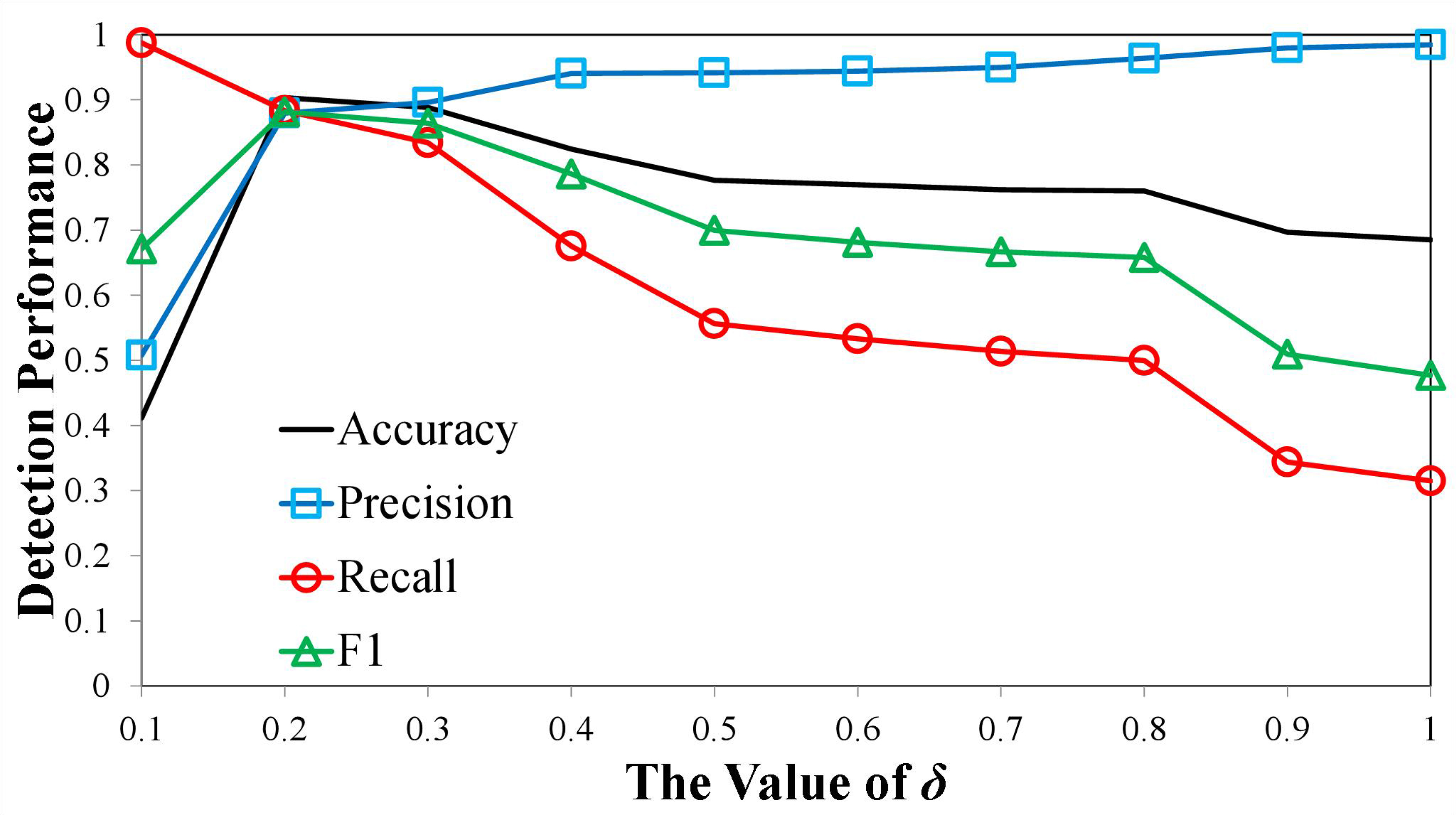
Figure 5. The effect of parameter δ.
4.4. Experiment 3: Ablation Experiment
To investigate the impact of the two data modalities (i.e., IoT sensing data and network traffic data) on anomaly-detection performance, we conducted separate tests on the autoencoder for IoT sensing data (IoT-AE) and the autoencoder for network traffic data (Network-AE). Here, IoT-AE was trained as a global autoencoder according to Section 3.3.1 without local autoencoders of the network traffic data. Similarly, Network-AE was trained as a global autoencoder without local autoencoders of the IoT sensing data.
In the first experiment, we compared IoT-AE with AD-FIT and other baseline methods as follows. These baseline methods consider only IoT sensing data.
MLP-IAE: An autoencoder-based anomaly detection model based only on IoT sensing data. It uses a two-layer MLP as the encoder and decoder.
LSTM-IAE: It is also an autoencoder-based anomaly detection model based only on IoT sensing data. It uses a two-layer stacked LSTM as the encoder and decoder.
MTGNN: This is a prediction-based anomaly detection model. Specifically, it first trains a multivariate time-series prediction model based on a novel GNN proposed in[59], and then detects anomalies by comparing the predicted values and the true values.
The experimental results are shown in Table 2. First, LSTM-IAE, MTGNN, and IoT-AE achieve better performance than MLP-IAE. This indicates that temporal patterns are crucial for IoT sensing data-based anomaly detection, and therefore should not be ignored. Second, IoT-AE has a slight advantage over LSTM-IAE. This result shows that using a graph to capture spatial correlations across dimensions of multivariate time-series data benefits anomaly detection. Third, MTGNN performs worse than LSTM-IAE. MTGNN detects anomalies by predicting the value at a given time point and comparing it with the observed value at that time point. The prediction-based anomaly detection model evaluates prediction error at a single time point, while the autoencoder-based anomaly detection model evaluates reconstruction error over a time range. This suggests that a large proportion of anomalies in our dataset are subtle and collectively evolving trend anomalies, rather than significant value changes at a given time point.
The evaluation of the autoencoder for IoT sensing data
| Accuracy | Precision | Recall | F1 | |
| MLP-IAE | 0.701 | 0.595 | 0.837 | 0.696 |
| LSTM-IAE | 0.855 | 0.776 | 0.906 | 0.836 |
| MTGNN | 0.829 | 0.795 | 0.783 | 0.788 |
| IoT-AE | 0.865 | 0.821 | 0.853 | 0.837 |
| AD-FIT | 0.903 | 0.879 | 0.883 | 0.881 |
In the second experiment, we compared Network-AE with AD-FIT and other baseline methods as follows. These baseline methods consider only network traffic data. We extracted statistical features according to Section 3.2.2 as the input to these baseline methods.
iForest: The iForest model was trained using only network traffic data.
MLP-NAE: An autoencoder-based anomaly detection model trained only on network traffic data. It uses a two-layer MLP as the encoder and decoder.
The experimental results are shown in Table 3. First, deep-learning-based models (i.e., MLP-NAE and Network-AE) outperform traditional machine-learning-based models (i.e., iForest). This finding is consistent with the results of the previous experiment presented in Section 4.2. Second, Network-AE outperforms MLP-NAE. It demonstrates the advantages of model ensemble, which can reduce the risk of overfitting. Finally, AD-FIT achieves the best overall performance among the evaluated baseline methods. It demonstrates the advantages of multi-view data fusion.
Evaluation of the autoencoder on network traffic data
| Accuracy | Precision | Recall | F1 | |
| iForest | 0.751 | 0.799 | 0.517 | 0.628 |
| MLP-NAE | 0.762 | 0.635 | 0.974 | 0.769 |
| Network-AE | 0.901 | 0.967 | 0.784 | 0.865 |
| AD-FIT | 0.903 | 0.879 | 0.883 | 0.881 |
4.5. Experiment 4: Case Study
In this section, we use three cases to demonstrate the effectiveness of AD-FIT. Figure 6A and B present the IoT sensing data and network traffic data for Case 1, respectively; Figure 6C and D present the corresponding data for Case 2; and Figure 6E and F present the corresponding data for Case 3. For each case, the IoT sensing data comprise five dimensions (latitude, longitude, temperature, pressure, and humidity), and the network traffic data comprise six representative features.
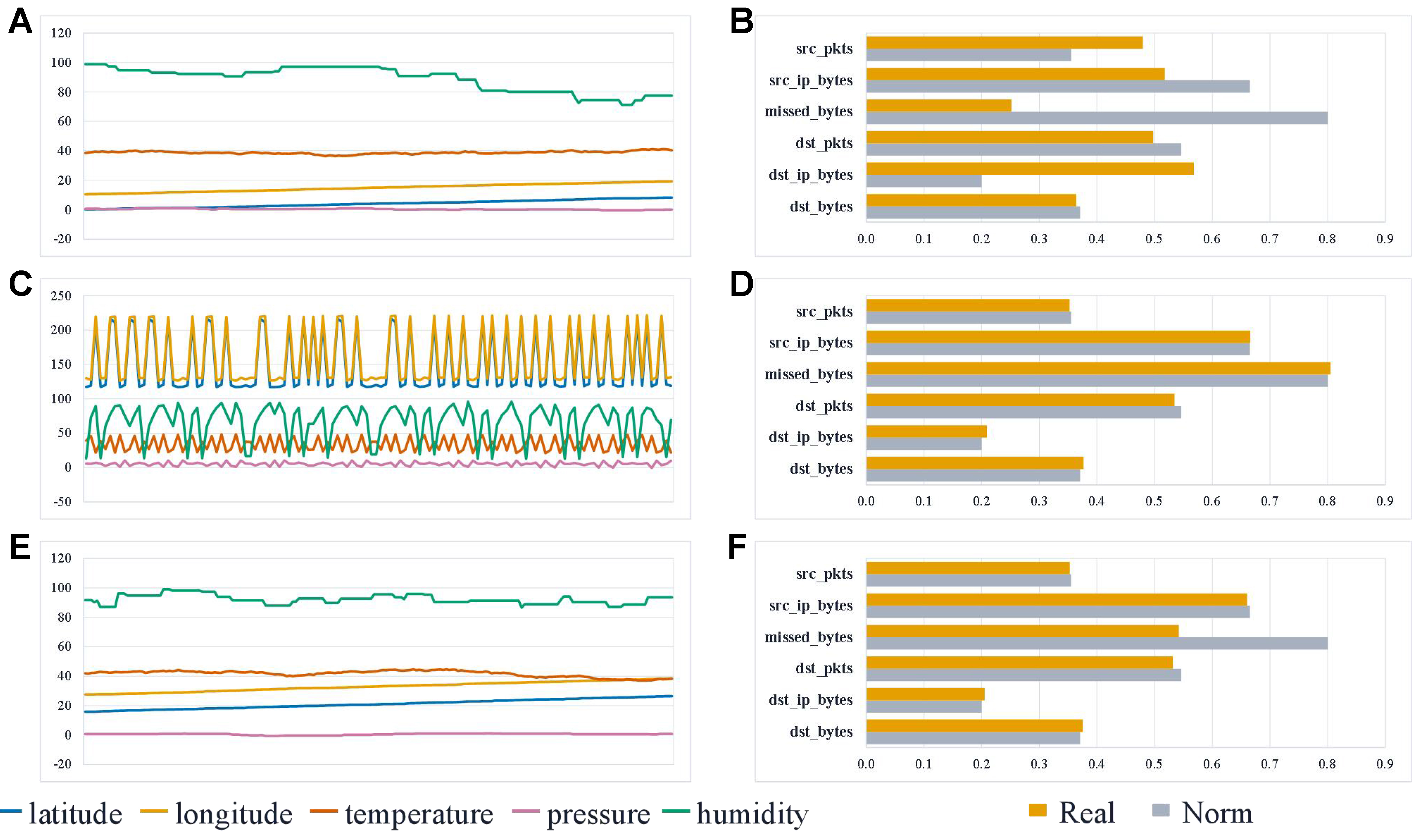
Figure 6. Representative cases illustrating the complementary roles of IoT sensing data and network traffic data in AD-FIT. (A) IoT sensing data of Case 1, which show no obvious deviation from normal patterns; (B) network traffic data of Case 1, which show significant deviations in multiple features; (C) IoT sensing data of Case 2, which show pronounced fluctuations; (D) network traffic data of Case 2, which show no obvious deviation from normal patterns; (E) IoT sensing data of Case 3, in which the humidity dimension shows a slight fluctuation; and (F) network traffic data of Case 3, in which the missed_bytes feature shows a slight deviation. IoT: Internet of Things.
The first case shows an abnormal sample that cannot be detected by considering only the IoT sensing data, since the five displayed IoT sensing dimensions show no obvious deviation from their normal patterns, as shown in Figure 6A. On the other hand, we can observe a significant deviation in most features of the network traffic data, as shown in Figure 6B, where “Norm” stands for the average value of a specific feature in all the normal samples and “Real” stands for the real value of the feature in the target sample. Here, dst_bytes, dst_ip_bytes, dst_pkts, missed_bytes, src_ip_bytes, and src_pkts denote bytes of packets received by the destination system, bytes of the IP header of the destination system, number of packets received by the destination system, bytes of missed packets, bytes of the IP header of the source system, and number of packets sent by the source system. As a result, this sample can be detected by an anomaly detector based on network traffic data. The second case shows the opposite scenario, where the network traffic data show almost no deviation across all features, while the IoT sensing data curve has pronounced fluctuations (as shown in Figure 6C and D). Therefore, this sample cannot be detected by an anomaly detector based on network traffic data alone but can be detected using IoT sensing data.
As shown in Figure 6E and F, the third case shows a more subtle anomalous sample, where neither IoT sensing data nor network traffic data exhibit significant deviations from normal temporal patterns. Nevertheless, the humidity dimension of the IoT sensing data and the missed_bytes feature of the network traffic data show slight fluctuations. By considering the two factors simultaneously, AD-FIT can successfully identify this abnormal sample, highlighting the advantage of the data fusion scheme.
5. CONCLUSIONS
In this paper, we investigate anomaly detection in IIoT systems. We propose AD-FIT, a novel unsupervised deep learning framework to identify anomalies by fusing multiple autoencoders based on the joint consideration of IoT sensing data and network traffic data in IIoT systems. By exploiting and learning the correlation patterns between multiple data modalities, AD-FIT achieves the best performance among the evaluated baseline methods on the ToN_IoT dataset.
Overall, the experimental results consistently demonstrate AD-FIT’s effectiveness. The comparison experiment shows that learning a global model from local autoencoder reconstruction errors is more effective than direct feature-level fusion or simple voting strategies. The parameter tuning experiment identifies an appropriate trade-off between precision and recall, while the ablation experiment confirms the complementary contributions of different data modalities. Finally, the case study further illustrates that jointly considering IoT sensing data and network traffic data enables AD-FIT to detect subtle anomalies that may be overlooked when either modality is used alone.
Future work will focus on two directions. First, AD-FIT detects anomalous events but does not classify them. Hence, equipping AD-FIT with anomaly classification capabilities could facilitate more effective responses to detected anomalies. Second, diagnosing detected anomalies and tracing their root causes are also important directions for future research.
DECLARATIONS
Authors’ contributions
Responsible for the overall study: Wang, F.
Wrote the manuscript: Lv, M.; Wang, F.
Contributed to the discussion and revision of the manuscript: Wang, L.; Chen, H.; Zhang, Z.; Tao, Y.
All authors read and approved the final manuscript.
Availability of data and materials
The data used in this paper are publicly available at https://research.unsw.edu.au/projects/toniot-datasets.
AI and AI-assisted tools statement
During revision of this manuscript, the authors used the AI tool ChatGPT (version GPT-5.6 Sol, released 2026-07-09) to edit the language and improve the clarity of the text. All AI-assisted suggestions were critically reviewed and edited by the authors, who take full responsibility for the final content. No AI-assisted tools were used to generate experimental data, conduct experiments, or determine the research conclusions.
Financial support and sponsorship
The work is supported by the Shaoxing Science and Technology Plan Project (2025B11004), Quzhou Science and Technology Research Project (2025K132), National Natural Science Foundation of China (62372410), and the Key Technology Research and Development Program of Shandong Province (2024SZD1A11).
Conflicts of interest
Tao, Y. is affiliated with Shaoxing Smart City Group Co., LTD., while the other authors declare no conflicts of interest.
Ethical approval and consent to participate
Not applicable.
Consent for publication
Not applicable.
Copyright
© The author(s) 2026.
REFERENCES
1. Pang, G.; Shen, C.; Cao, L.; Hengel, A. V. D. Deep learning for anomaly detection: a review. ACM. Comput. Surv. 2022, 54, 1-38.
2. Omar, S.; Ngadi, A.; Jebur, H. H. Machine learning techniques for anomaly detection: an overview. Int. J. Comput. Appl. 2013, 79, 33-41.
3. Audibert, J.; Michiardi, P.; Guyard, F.; Marti, S.; Zuluaga, M. A. USAD: unsupervised anomaly detection on multivariate time series. In Proceedings of the 26th ACM SIGKDD International Conference on Knowledge Discovery & Data Min. Association for Computing Machinery; 2020. pp. 3395-404.
4. Singhal, A.; Seborg, D. E. Clustering multivariate time‐series data. J. Chemometrics. 2005, 19, 427-38.
5. Karim, S.; Rousanuzzaman, M.; Yunus, P. A.; Khan, P. H.; Asif, M. Implementation of K-means clustering for intrusion detection. Int. J. Sci. Res. Comput. Sci. Eng. Inf. Technol. 2019, 5, 1232-41.
6. Erfani, S. M.; Rajasegarar, S.; Karunasekera, S.; Leckie, C. High-dimensional and large-scale anomaly detection using a linear one-class SVM with deep learning. Pattern. Recognit. 2016, 58, 121-34.
7. Liu, F. T.; Ting, K. M.; Zhou, Z. H. Isolation forest. In 2008 Eighth IEEE International Conference on Data Mining, Pisa, Italy. Dec 15-19, 2008. IEEE; 2008. pp. 413-22.
8. Malhotra, P.; Ramakrishnan, A.; Anand, G.; Vig, L.; Agarwal, P.; Shroff, G. LSTM-based encoder-decoder for multi-sensor anomaly detection. arXiv 2016, arXiv:1607.00148. Available online: https://doi.org/10.48550/arXiv.1607.00148. (accessed 2026-09-21).
9. Zeng, F.; Chen, M.; Qian, C.; Wang, Y.; Zhou, Y.; Tang, W. Multivariate time series anomaly detection with adversarial transformer architecture in the Internet of Things. Future. Gener. Comput. Syst. 2023, 144, 244-55.
10. Nanduri, A.; Sherry, L. Anomaly detection in aircraft data using recurrent neural networks (RNN). In 2016 Integrated Communications Navigation and Surveillance (ICNS), Herndon, USA. Apr 19-21, 2016. IEEE; 2016. pp. 5C2-1-8.
11. Hwang, R.; Peng, M.; Huang, C.; Lin, P.; Nguyen, V. An unsupervised deep learning model for early network traffic anomaly detection. IEEE. Access. 2020, 8, 30387-99.
12. Dutta, V.; Pawlicki, M.; Kozik, R.; Choraś, M. Unsupervised network traffic anomaly detection with deep autoencoders. Log. J. IGPL. 2022, 30, 912-25.
13. Xu, W.; Jang-Jaccard, J.; Singh, A.; Wei, Y.; Sabrina, F. Improving performance of autoencoder-based network anomaly detection on NSL-KDD dataset. IEEE. Access. 2021, 9, 140136-46.
14. Said Elsayed, M.; Le-Khac, N. A.; Dev, S.; Jurcut, A. D. Network anomaly detection using LSTM based autoencoder. In Proceedings of the 16th ACM Symposium on QoS and Security for Wireless and Mobile Networks. Association for Computing Machinery; 2020. pp. 37-45.
15. Zare, F.; Mahmoudi-Nasr, P.; Yousefpour, R. A real-time network based anomaly detection in industrial control systems. Int. J. Crit. Infrastruct. Prot. 2024, 45, 100676.
16. Xu, J.; Wu, H.; Wang, J.; Long, M. Anomaly transformer: time series anomaly detection with association discrepancy. In ICLR 2022 Conference. 2022. https://openreview.net/forum?id=LzQQ89U1qm_. (accessed 2026-09-21).
17. Tuli, S.; Casale, G.; Jennings, N. R. TranAD: deep transformer networks for anomaly detection in multivariate time series data. Proc. VLDB. Endow. 2022, 15, 1201-14.
18. Zhang, W.; Zhang, C.; Tsung, F. GRELEN: multivariate time series anomaly detection from the perspective of graph relational learning. In Proceedings of the Thirty-First International Joint Conference on Artificial Intelligence (IJCAI-22). 2022. pp. 2390-7.
19. Zhou, Q.; Chen, J.; Liu, H.; He, S.; Meng, W. Detecting multivariate time series anomalies with zero known label. Proc. AAAI. Conf. Artif. Intell. 2023, 37, 4963-71.
20. Song, J.; Kim, K.; Oh, J.; Cho, S. MEMTO: memory-guided transformer for multivariate time series anomaly detection. In Proceedings of the 37th International Conference on Neural Information Processing Systems. Curran Associates Inc.; 2023. pp. 57947-63.
21. Wang, C.; Zhuang, Z.; Qi, Q.; et al. Drift doesn’t matter: dynamic decomposition with diffusion reconstruction for unstable multivariate time series anomaly detection. In Proceedings of the 37th International Conference on Neural Information Processing Systems. Curran Associates Inc.; 2023. pp. 10758-74.
22. Dai, Z.; He, L.; Yang, S. H.; Leeke, M. SARAD: spatial association-aware anomaly detection and diagnosis for multivariate time series. In Proceedings of the 38th International Conference on Neural Information Processing Systems. Curran Associates Inc.; 2024. pp. 48371-410.
23. Huang, X.; Chen, W.; Hu, B.; Mao, Z. Graph mixture of experts and memory-augmented routers for multivariate time series anomaly detection. Proc. AAAI. Conf. Artif. Intell. 2025, 39, 17476-84.
24. Liu, S.; Kimura, T.; Liu, D.; et al. FOCAL: contrastive learning for multimodal time-series sensing signals in factorized orthogonal latent space. In Proceedings of the 37th International Conference on Neural Information Processing Systems. Curran Associates Inc.; 2023. pp. 47309-38.
25. Ferrag, M. A.; Friha, O.; Hamouda, D.; Maglaras, L.; Janicke, H. Edge-IIoTset: a new comprehensive realistic cyber security dataset of IoT and IIoT applications for centralized and federated learning. IEEE. Access. 2022, 10, 40281-306.
26. Neto, E. C. P.; Dadkhah, S.; Ferreira, R.; Zohourian, A.; Lu, R.; Ghorbani, A. A. CICIoT2023: a real-time dataset and benchmark for large-scale attacks in IoT environment. Sensors 2023, 23, 5941.
27. Qathrady, M. A.; Ullah, S.; Alshehri, M. S.; et al. SACNN‐IDS: a self‐attention convolutional neural network for intrusion detection in industrial Internet of Things. CAAI. Trans. Intell. Technol. 2024, 9, 1398-411.
28. Li, X.; Li, S.; Zhang, G.; Xie, Y.; Wang, T.; Chu, F. A novel interpretable dynamic weighted domain adaptation network for cross-domain fault diagnosis of bearings under time-varying speeds. Eng. Appl. Artif. Intell. 2026, 170, 114173.
29. Griffin, J. M.; Doberti, A. J.; Hernández, V.; Miranda, N. A.; Vélez, M. A. Multiple classification of the force and acceleration signals extracted during multiple machine processes: part 1 intelligent classification from an anomaly perspective. Int. J. Adv. Manuf. Technol. 2017, 93, 811-23.
30. Janssens, O.; Slavkovikj, V.; Vervisch, B.; et al. Convolutional neural network based fault detection for rotating machinery. J. Sound. Vib. 2016, 377, 331-45.
31. Amruthnath, N.; Gupta, T. A research study on unsupervised machine learning algorithms for early fault detection in predictive maintenance. In 2018 5th International Conference on Industrial Engineering and Applications (ICIEA), Singapore. Apr 26-28, 2018. IEEE; 2018. pp. 355-61.
32. Diez-Olivan, A.; Pagan, J. A.; Khoa, N. L. D.; Sanz, R.; Sierra, B. Kernel-based support vector machines for automated health status assessment in monitoring sensor data. Int. J. Adv. Manuf. Technol. 2018, 95, 327-40.
33. Joshi, S. S.; Phoha, V. V. Investigating hidden Markov models capabilities in anomaly detection. In Proceedings of the 43rd Annual ACM Southeast Conference. Association for Computing Machinery; 2005. pp. 98-103.
34. Nguyen, M. N.; Vien, N. A. Scalable and interpretable one-class SVMs with deep learning and random fourier features. In Berlingerio, M.; Bonchi, F.; Gärtner, T.; Hurley, N.; Ifrim, G.; eds. Machine learning and knowledge discovery in databases. Cham: Springer International Publishing; 2019. pp. 157-72.
35. Xu, H.; Chen, W.; Zhao, N.; et al. Unsupervised anomaly detection via variational auto-encoder for seasonal KPIs in web applications. In Proceedings of the 2018 World Wide Web Conference. International World Wide Web Conferences Steering Committee; 2018. pp. 187-96.
36. Lu, C.; Wang, Z.; Qin, W.; Ma, J. Fault diagnosis of rotary machinery components using a stacked denoising autoencoder-based health state identification. Signal. Process. 2017, 130, 377-88.
37. Zhang, C.; Song, D.; Chen, Y.; et al. A deep neural network for unsupervised anomaly detection and diagnosis in multivariate time series data. Proc. AAAI. Conf. Artif. Intell. 2019, 33, 1409-16.
38. Yin, C.; Zhang, S.; Wang, J.; Xiong, N. N. Anomaly detection based on convolutional recurrent autoencoder for IoT time series. IEEE. Trans. Syst. Man. Cybern. Syst. 2022, 52, 112-22.
39. Muneer, A.; Mohd Taib, S.; Mohamed Fati, S.; Balogun, A. O.; Abdul Aziz, I. A hybrid deep learning-based unsupervised anomaly detection in high dimensional data. Comput. Mater. Contin. 2022, 70, 5363-81.
40. Zheng, Y. Methodologies for cross-domain data fusion: an overview. IEEE. Trans. Big. Data. 2015, 1, 16-34.
41. Xiao, X.; Zheng, Y.; Luo, Q.; Xie, X. Inferring social ties between users with human location history. J. Ambient. Intell. Human. Comput. 2014, 5, 3-19.
42. Ngiam, J.; Khosla, A.; Kim, M.; Nam, J.; Lee, H.; Ng, A. Y. Multimodal deep learning. In Proceedings of the 28th International Conference on Machine Learning, Bellevue, USA. 2011. pp. 689-96. https://ai.stanford.edu/~jngiam/papers/NgiamKhoslaKimNamLeeNg2011.pdf. (accessed 2026-09-21).
43. Nagrani, A.; Yang, S.; Arnab, A.; Jansen, A.; Schmid, C.; Sun, C. Attention bottlenecks for multimodal fusion. arXiv 2021, arXiv:2107.00135. Available online: https://doi.org/10.48550/arXiv.2107.00135. (accessed 2026-09-21).
44. Yasaei, R.; Moghaddas, Y.; Al Faruque, M. A. IoT-GRAF: IoT graph learning-based anomaly and intrusion detection through multi-modal data fusion. In 2024 Design, Automation & Test in Europe Conference & Exhibition (DATE), Valencia, Spain. Mar 25-27, 2024. IEEE; 2024. p. 1-6.
45. Zhan, D.; Zhang, W.; Ye, L.; Yu, X.; Zhang, H.; He, Z. Anomaly detection in industrial control systems based on cross-domain representation learning. IEEE. Trans. Dependable. Secure. Comput. 2025, 22, 2505-18.
46. Sun, Y.; Qi, J.; Zheng, Y.; Zhang, R. K-nearest neighbor temporal aggregate queries. In Proceedings of the 18th International Conference on Extending Database Technology. 2015. pp. 493-504. https://www.microsoft.com/en-us/research/publication/k-nearest-neighbor-temporal-aggregate-queries/. (accessed 2026-09-21).
47. Canonico, R.; Esposito, G.; Navarro, A.; Romano, S. P.; Sperlì, G.; Vignali, A. Empowered cyber–physical systems security using both network and physical data. Comput. Secur. 2025, 152, 104382.
48. Pinto, A.; Herrera, L.; Donoso, Y.; Gutierrez, J. A. Cyber-physical anomaly detection a deep adversarial fusion of sensor and network data. Discov. Comput. 2026, 29, 10064.
49. Shafin, S. S.; Karmakar, G.; Mareels, I.; Balasubramanian, V.; Kolluri, R. R. Sensor self-declaration of numeric data reliability in Internet of Things. IEEE. Trans. Reliab. 2025, 74, 2751-65.
50. Veličković, P.; Cucurull, G.; Casanova, A.; Romero, A.; Liò, P.; Bengio, Y. Graph attention networks. arXiv 2017, arXiv:1710.10903. Available online: https://doi.org/10.48550/arXiv.1710.10903. (accessed 2026-09-21).
52. Ngo, G.; Beard, R.; Chandra, R. Evolutionary bagging for ensemble learning. Neurocomputing 2022, 510, 1-14.
53. Kadkhodaei, H. R.; Moghadam, A. M. E.; Dehghan, M. HBoost: a heterogeneous ensemble classifier based on the boosting method and entropy measurement. Expert. Syst. Appl. 2020, 157, 113482.
54. Zhang, H.; Li, J.; Liu, X.; Dong, C. Multi-dimensional feature fusion and stacking ensemble mechanism for network intrusion detection. Future. Gener. Comput. Syst. 2021, 122, 130-43.
55. Kuncheva, L. I.; Whitaker, C. J. Measures of diversity in classifier ensembles and their relationship with the ensemble accuracy. Mach. Learn. 2003, 51, 181-207.
56. Booij, T. M.; Chiscop, I.; Meeuwissen, E.; Moustafa, N.; Hartog, F. T. H. D. ToN_IoT: the role of heterogeneity and the need for standardization of features and attack types in IoT network intrusion data sets. IEEE. Internet. Things. J. 2022, 9, 485-96.
57. Sokolova, M.; Lapalme, G. A systematic analysis of performance measures for classification tasks. Inf. Process. Manag. 2009, 45, 427-37.
58. Li, R.; Li, Y.; He, W.; Chen, L.; Luo, J. Multi-layer reconstruction errors autoencoding and density estimate for network anomaly detection. Comput. Model. Eng. Sci. 2021, 128, 381-97.
59. Wu, Z.; Pan, S.; Long, G.; Jiang, J.; Chang, X.; Zhang, C. Connecting the dots: multivariate time series forecasting with graph neural networks. In Proceedings of the 26th ACM SIGKDD International Conference on Knowledge Discovery & Data Mining. Association for Computing Machinery; 2020. pp. 753-63.
Cite This Article
 Open Access
How to Cite
Wang, F.; Wang, L.; Lv, M.; Chen, H.; Zhang, Z.; Tao, Y. AD-FIT: industrial anomaly detection via fusion of IoT sensing and network traffic data. Intell. Robot. 2026, 6(3), 729-49. https://dx.doi.org/10.20517/ir.2026.32
Download Citation
If you have the appropriate software installed, you can download article citation data to the citation manager of your choice. Simply select your manager software from the list below and click on download.
Export Citation File
Type of Import
Tips on Downloading Citation
Citation Manager File Format
Type of Import
Direct Import: When the Direct Import option is selected (the default state), a dialogue box will give you the option to Save or Open the downloaded citation data. Choosing Open will either launch your citation manager or give you a choice of applications with which to use the metadata. The Save option saves the file locally for later use.
Indirect Import: When the Indirect Import option is selected, the metadata is displayed and may be copied and pasted as needed.
About This Article
Copyright

Data & Comments
Data
0










Comments
Comments must be written in English. Spam, offensive content, impersonation, and private information will not be permitted. If any comment is reported and identified as inappropriate content by OAE staff, the comment will be removed without notice. If you have any queries or need any help, please contact us at [email protected].