


Risk-adaptive conservation zones: integrating degradation vulnerability into spatially explicit carbon crediting
 0
0 
Abstract
Fragmentation and edge exposure have caused major, spatially structured carbon losses in once-intact forests globally, yet most carbon methodologies, though central to conservation finance, still rely primarily on projected deforestation and fail to explicitly capture degradation-driven losses spatially. Here, we develop a Risk-Adaptive Conservation Zone (RACZ) model that integrates landscape ecology, spatial gradients of deforestation, and mechanistic edge-effect dynamics to delineate evidence-based carbon crediting zones. Using the distance to the nearest deforestation as a proxy for spatial risk, and incorporating pressure intensity and landscape structure, the model generates a dynamic, project-specific RACZ that adapts to both external pressure and internal resistance. Two tropical, similarly sized areas with contrasting deforestation pressures were tested. The model yielded a small RACZ of 1,150 ha in the intact, low-pressure landscape, concentrated in narrow bands near isolated edges, covering 0.27% of the total area. While for the highly fragmented frontier, RACZ expanded to 337,985 ha, covering 99.4% of the total area and reflecting pervasive, far-reaching degradation risk. These results show that RACZ restricts crediting to genuinely vulnerable areas in intact regions while capturing extensive risk in heavily fragmented frontiers. Therefore, this ecologically grounded approach complements core principles of the Integrity Council for the Voluntary Carbon Market by improving environmental integrity and credibility in carbon accounting through aligning credit zones with spatial degradation risk.
Keywords
INTRODUCTION
Nature-based climate solutions, particularly the conservation and restoration of forests, are recognized as a cornerstone of any viable strategy to meet the climate mitigation targets, with the potential to provide over a third of the cost-effective CO2 mitigation needed by 2030[1]. In terms of conservation scope, most methodologies still treat deforestation as the most relevant disturbance and assume that emissions occur only where forests are directly cleared. Most carbon accounting frameworks such as REDD+ have mainly focused on projecting deforestation to define highly flexible, while easily inflated, baselines[1-4], which are often based on simple correlations or historical transitions rather than ecological processes[5]. Of the deforestation baselines found to be inflated, only 25% of the resulting avoided-deforestation credits led to actual emission reductions[5,6].
Recent commentaries and syntheses argue that restoring trust in carbon markets requires more transparent and evidence-based quantification[4]. This matters “now” because carbon market legitimacy has become a binding constraint: when integrity is questioned, demand softens, pricing becomes volatile, and high-quality projects struggle to compete in an increasingly skeptical environment. Recent market analyses indicate that high-integrity credits typically trade at price premiums of three to five times those of lower-quality offsets—often around US$ 15 t-1CO2 compared to US$ 3-5 t-1CO2—reflecting buyer preference for reduced uncertainty and more defensible climate claims[7,8]. Parallel methodological critiques identify structural reasons for inflated crediting under commonly used REDD+ baseline approaches[9,10]. Approximately 78% of over-crediting is due to the various ex ante modeling approaches used in certified valuations, with considerable uncertainty surrounding this allocation being acknowledged[4,11]. Together, these studies highlight the same practical point for developers and standards: credibility increasingly relies on whether a method can distinguish truly threatened forests from relatively stable ones and assign credit accordingly.
A central gap emerges at the interface between current ecological understanding and operational carbon methodologies. Most REDD+ approaches estimate avoided emissions primarily by projecting future deforestation and applying risk models tuned to the probability of forest loss. That logic is appropriate for deforestation, but it tends to treat remaining forest as uniformly “safe” unless it is predicted to be cleared—thereby under-representing a second, increasingly well-documented pathway of carbon loss: degradation inside standing forests driven by fragmentation and proximity to anthropogenic edges. Carbon losses derived from the edge effect induced by fragmentation affect 97% of global forest area[12,13] and may account for up to one-third of losses resulting from deforestation[14]. Consequently, forests adjacent to deforested regions can function as chronic sources of carbon emissions, with cumulative biomass losses working as an additional unquantified flux, that can counteract carbon emissions avoided by reducing deforestation[14,15]. Indeed, studies have demonstrated that degradation is not a peripheral or secondary impact but rather a primary driver of carbon loss, potentially exceeding emissions from deforestation[16,17].
This effect is not fortuitous. A growing body of empirical evidence shows that forest degradation driven by proximity to deforestation has substantial impacts on biodiversity, vegetation structure, and aboveground biomass[18-22]. Edge-induced microclimatic changes—such as increased temperature, reduced humidity, and greater wind exposure—elevate physiological stress and mortality among large, high-biomass trees, leading to shifts in species composition, lower wood density, reduced carbon storage, and declining ecosystem function[23-25]. These effects commonly penetrate tens to hundreds of meters into forest interiors, depending on fragment size, shape, and landscape configuration[20,26,27], and often persist over decadal timescales due to repeated edge exposure and structural instability[14,28,29].
Landscape ecology provides a mechanistic explanation for how degradation occurs, depending critically on landscape structure, including fragment size, shape, and connectivity[30,31]. These attributes modulate the spatial spread of ecological disturbances, producing predictable distance-decay patterns across forest mosaics[32,33]. In practical terms, two projects with identical “forest area” may have sharply different carbon trajectories depending on how fragmented they are and how exposed their boundaries are to the surrounding matrix—precisely the type of within-project heterogeneity that deforestation-only baselines struggle to represent[24,34]. While typical REDD+ approaches identify how much deforestation is likely to occur, they fail to capture the spatial pattern of disturbance propagation and the ecological vulnerability that emerges from the area's characteristics and landscape context.
The influence of external disturbances typically diminishes with distance from their source due to barriers, habitat heterogeneity, and energy dissipation, producing nonlinear distance-decay patterns[35,36]. Accordingly, edge effects, microclimatic alterations, and other disturbance signals are commonly represented using exponential or exponential-like functions[27,33,37,38]. Building on these principles, we developed a Risk-Adaptive Conservation Zone (RACZ) model to delineate carbon crediting areas based on spatially structured degradation risk. It captures the asymmetric and scale-dependent nature of edge-driven degradation, while providing a mechanistic representation of how landscape structure mediates ecological responses, rather than relying on purely statistical association[32,33]. This study shows that RACZ identifies where forest carbon is plausibly threatened by deforestation-driven degradation, thus supporting conservative and transparent decisions consistent with Integrity Council for the Voluntary Carbon Market (ICVCM) principles on additionality, permanence, and robust quantification.
METHODS
RACZ model is a distance-dependent, ecologically informed framework. It integrates: (i) delineation of a reference region (RR) surrounding the project area; (ii) quantification of external deforestation pressure; (iii) distance-dependent risk modelling; and (iv) parametrization based on mechanistic principles governed by landscape ecology. The model yields a dynamic internal buffer whose size varies locally in response to both the spatial gradient of surrounding deforestation and the structural vulnerability of the project area.
Distance-dependent risk model
Degradation risk is modelled using a truncated exponential decay function [Figure 1], where the independent variable d represents the Euclidean distance from the project boundary to the nearest deforested pixel. This exponential formulation follows well-established distance-decay relationships in landscape ecology, where the intensity of ecological processes decreases as a function of distance from disturbance sources[27,30,39]. Empirical studies have consistently shown that proximity to forest edges influences microclimatic conditions, biomass dynamics, and biodiversity patterns, with effects attenuating nonlinearly with the distance[20,40,41].
Figure 1. Conceptual illustration for truncated exponential decay function for α = 5 m. When d > α, R(d) = 0; when d = 0, R(d) = 5. The dataset and graphic were generated in Python using NumPy and Matplotlib. Note: The scale of the figure is an approximation.
In this analysis, the dependent variable (R(d)) is the buffer radius, calculated for each point along the project edge, from which a risk zone of variable size is defined.
Where:
• R(d) is the buffer radius, defining the internal limit of degradation risk, expressed in meters;
• α is the maximum distance of anthropogenic matrix influence within the project area, expressed in meters;
• β is the exponential decay rate, governing how rapidly the influence attenuates with distance, expressed in m-1.
• d is the distance between each point on the edge of the project area and the nearest deforested area within the landscape, expressed in meters;
•
The truncation ensures that external influence is bounded by a biologically plausible maximum distance, beyond which effects are assumed negligible. When d = 0 (minimum possible distance), the influence reaches its maximum (R(d) = α); when d > α, influence decays to zero. The model’s behavior is illustrated in Figure 1, which is based on hypothetical data.
This nearest-distance model is particularly applicable in landscapes where deforestation constitutes the primary and spatially continuous disturbance driver, exhibiting spatial autocorrelation and predominantly isotropic edge effects, such that distance to the nearest deforestation serves as a conservative proxy for degradation exposure.
Parametrization of the model
The exponential decay model arises as the analytical solution of a first-order differential equation describing the proportional decay with distance, a property characteristic of diffusion-like ecological processes. As the exponential decay model is grounded in well-established mathematical properties of diffusion, attenuation, and boundary-driven processes, the parameters α and β are defined theoretically[35,42].
Within this formulation, parameters emerge from the mathematical structure of the differential equation and from ecological first principles that govern the structure and dynamics of the landscape, not from data calibration. This is consistent with mechanistic modeling in landscape ecology, where parameters are derived from theoretical descriptions of spatial propagation, edge influence, fragment geometry, and landscape resistance, rather than solely from empirical regression.
Alpha (α): maximum distance of influence
The parameter α represents the maximum spatial extent of degradation influence generated by surrounding deforestation. It is interpreted as the upper bound of edge-driven degradation pressure acting on the project area. Alpha is obtained from the following steps: (i) RR delineation; (ii) Building of a binary matrix with deforestation data; (iii) Computing a Euclidean distance surface; (iv) Estimation of the Weighted Landscape Class Proportion (PLw); and (v) Applying the equation to estimate the alpha.
• Reference region delineation
The RR is defined as a buffer surrounding the project area, with radius scaled to project size. It provides the spatial data needed to set the parameters for the variable internal RACZ. The radius of the RR is calculated using a geometric expression that scales proportionally to the project area, ensuring consistent spatial representation of potential threats in different project contexts.
Where:
• RRradius is the buffer radius of the RR, expressed in meters;
• PA is the project area, expressed in square meters.
The term (PA/2) establishes a sufficiently large reference radius to capture the surrounding landscape context while avoiding an excessive spatial extent that would dilute the representation of local pressure.
Based on the calculated radius, we define an outer buffer zone to represent a RR, from which the data used to quantify external deforestation pressure is obtained.
• Binary matrix
We generated a binary land-cover matrix representing the presence or absence of deforestation within the RR, to quantify the spatial influence of deforestation over the area. Under this framework, deforestation refers to the current state of land cover, based on stable anthropogenic land-use classes, defined as the long-term or permanent conversion of forested land into non-forested land as a result of human activities. For this analysis, we used the land use and land cover (LULC) mapping from the MapBiomas platform, collection 10 (launched in August 2025) for 2024[43]. MapBiomas provides annual, wall-to-wall LULC classifications for Brazil, based on the Random Forest algorithm for processing Landsat images, with a resolution of 30 m[44].
The MapBiomas dataset was subsequently reclassified into a binary deforestation matrix, in which anthropogenic land uses are assigned a value of 1 (deforested), while all remaining land-cover classes are assigned a value of 0 (non-deforested). The resulting matrix serves as the fundamental layer from which we calculate the Euclidean distance (d) to the nearest deforested pixel, generating a continuous "distance to deforestation" surface. This distance raster is then used in the remaining steps.
• Euclidean distance
After generating the binary deforestation matrix, the next preparatory step consists of computing Euclidean distance surface to quantify how far each location within the study area lies from the nearest deforested pixel. The Euclidean distance algorithm measures the shortest straight-line distance between every non-deforested cell (value 0) and the nearest cell classified as deforested (value 1), producing a continuous raster in which each pixel contains a distance value expressed in map units. This approach follows the standard convention in landscape ecology, where proximity to edges and disturbance sources is represented as straight-line distance due to its geometric clarity and established empirical performance[27,33,37]. Because edge influence and degradation processes tend to diffuse outward from deforestation boundaries in approximately radial patterns, distance, from Euclidean distance algorithm, has long been recognized as the most appropriate metric for capturing spatial exposure to anthropogenic pressure[19,30,38]. The resulting distance raster captures the spatial gradient of deforestation intensity and, in addition to being used to determine alpha, serves as the main input variable (d) for the exponential degradation model.
• Weighted landscape class proportion (PLw)
The Weighted Landscape Class Proportion (PLw) is an original metric proposed in this study, designed to quantify deforestation pressure, in terms of magnitude and proximity, by integrating class proportion with a distance-based weighting function. It is constructed to translate the quantity and spatial configuration of deforestation within the RR into an effective measure of external anthropogenic pressure.
The calculation of the PLw is performed based on the following steps:
(i) Creation of a weight raster w(d), in which each pixel receives an individual weight based on its distance from the edge (Euclidean distance). To achieve this, the RR is divided into concentric circles reflecting the spatial distribution of deforestation in terms of the distance of each deforested pixel from the project edge. Each deforested pixel then receives a weight from 1 at the edge of the project to 0 at the outer limit of the ring, decaying with distance.
Where:
• w(di) is the distance-based weight assigned to pixel i, (unitless);
• di is the Euclidean distance between the deforested pixel i and the project boundary, expressed in meters;
• RRradius is the buffer radius of the RR, expressed in meters.
The result provides a spatial representation of the landscape structure, based on deforestation distribution.
(ii) Estimation of a weighted average that favors what is closest to the edge, regardless of the geometry or size of the RR.
Where:
• PLw is the Weighted Landscape Class Proportion, ranging from 0 to 1 (unitless);
• w(di) is the distance-based weight assigned to pixel i, unitless;
• n is the total number of pixels within the RR;
• bi is a binary variable equal to 1 if pixel i is deforested and 0 otherwise.
Lower PLw values reflect negligible or spatially distant deforestation relative to the project boundary, whereas higher values denote greater deforestation intensity and increasing edge-proximal concentration.
Unlike a simple proportional metric, PLw captures not only how much deforestation exists in the surrounding landscape, but also how spatially proximate it is to the project area, thereby providing a more meaningful representation of pressure gradients.
• Estimation of the alpha
The parameter α defines the maximum extent to which degradation can spread from the edge of a project area. Its value is derived empirically by applying a pressure adjustment factor (Fp) to the radius of the RR (RRradius) (see Equation 5), ensuring that α responds proportionally to the level of external disturbances to which the area is exposed. Ultimately, α represents the structural attributes of the landscape in the surroundings of the area, in relation to the deforestation class.
Where:
• α is the maximum spatial extent over which external anthropogenic pressure exerts influence on the Project Area, expressed in meters;
• RR is the radius is the radius of the RR, expressed in meters;
• Fp is the pressure adjustment factor, unitless.
BETA (β): decay rate of degradation influence
The parameter β controls the rate at which the degradation influence attenuates with distance in the exponential model. It represents the structural susceptibility of the forested landscape to edge-driven degradation and is determined by fragment size and fragment shape[40], two well-established controls on edge exposure and core-area buffering in landscape ecology. Fragments with higher edge-to-area ratios, typically associated with smaller size or irregular geometry, are more exposed to external influences and therefore, exhibit a smoother decay curve (lower β). Conversely, larger or more compact habitats show steeper attenuation of pressure (higher β). In these formulations, β acts as a modulator of the response, reflecting the degree of ecological resilience or susceptibility of the landscape to external stress.
Operationally, beta is obtained from two independent components:
(i) a shape-based circularity index (CI), representing geometric exposure to edge effects; and
(ii) an area-based resistance factor (k), representing the buffering effect of fragment size.
• Circularity index (CI)
Fragment shape is quantified using the CI, a dimensionless metric that relates area to perimeter and provides a proxy for edge susceptibility[45]. Shape metrics are strongly linked to fragmentation and edge exposure[33]. CI measures how closely a fragment approximates a perfect circle, which minimizes edge length for a given area.
Where:
• CI is the circularity index, unitless;
• A is the project area, expressed in square meters;
• p is the project perimeter, expressed in meters.
CI ranges from 0 to 1. Values approaching 1 indicate compact geometries with low edge exposure, while values near 0 indicate elongated or irregular shapes with high edge density and increased susceptibility to external disturbance.
• Area factor (k)
Fragment size influences degradation dynamics primarily through the proportion of interior (core) habitat because no standardized size index exists at the single-fragment level[41]. We defined an area factor (k) that captures the buffering capacity associated with fragment size. The relationship between area (A) and factor (k) is monotonically increasing and non-linear in nature—that is, larger areas have higher k values, but with decreasing growth (smaller marginal gains as A increases). This behavior is represented using a smooth, continuous function derived from monotonic cubic Hermite interpolation by segments (splines)[46], following established approaches for preserving monotonicity in ecological scaling[47]. k(A) is defined as the continuous function interpolated in logarithmic space, from previously defined anchor points.
Where:
• k(A) is the area factor, unitless;
• A is the project area, expressed in the same units used to define the anchor points;
• f is a monotonic cubic Hermite spline function fitted to predefined anchor points in log-area space.
This formulation yields a continuous, analytically tractable estimate of k for each project, avoiding discontinuities at class boundaries, and allows recalibration if additional reference points are introduced [Figure 2].
Figure 2. Continuous relationship between project area (A) and area factor (k). The curve of the equation and the graphic were generated in R, from ggplot package.
• Estimation of beta
The parameter β integrates the effects of fragment size and shape into a single structural control on degradation propagation. This combination allows β to reflect both a fragment's intrinsic capacity to dampen disturbances (area factor) and its geometric propensity to amplify edge effects (CI), resulting in a biologically significant and landscape-responsive parameter in the exponential degradation model.
Beta is calculated as:
Where:
• β is the decay rate of the exponential model, expressed in m-1;
• β0 is a scaling coefficient to preserve dimensional consistency, expressed in m-1;
• k is the Area Factor, unitless;
• CI is the circularity index, unitless.
The parameters CI and k are descriptors of the area’s structure and do not carry spatial units. Their role in the model is to modulate the rate at which the influence of external pressure decays across space. The dimensional component of the decay parameter is provided by β0. This formulation allows the model to maintain dimensional consistency while preserving its ecological interpretation as a measure of its susceptibility to degradation.
Mathematically, the equation ensures that β decreases with both a decrease in project area and an increase in shape irregularity (i.e., lower CI). Conversely, beta increases as the project area grows and CI increases. Consequently, lower decay rates are produced in structurally susceptible areas, while higher rates are produced in more stable areas.
Application of the model
The RACZ framework was applied to two contrasting case-study landscapes to demonstrate model behavior under differing disturbances. In both cases, land-cover data were reclassified into a binary deforestation matrix, from which Euclidean distance-to-deforestation surfaces were generated and used as inputs to the exponential degradation model.
The first case represents a low-pressure landscape, characterized by limited surrounding deforestation and weak fragmentation dynamics. The second represents a high-pressure frontier landscape, where extensive deforestation generates strong spatial gradients of degradation risk. Together, these cases demonstrate the flexibility, scalability, and structural sensitivity of the RACZ framework.
Case study 1: low anthropogenic pressure
Case study 1 [Figure 3] is a tropical forest called Kokolopori Bonobo Natural Reserve, located between the provinces of Tshuapa and Tshopo in the Democratic Republic of Congo, within the Congo Basin tropical rainforest, part of the Afrotropical moist broadleaf forest biome. The region lies in the Af classification of the Köppen-Geiger system and is characterized by high precipitation, consistently high temperatures, and the absence of a dry season. These conditions sustain dense evergreen forests with high biomass and complex vertical structure, forming part of one of the largest contiguous tropical forests in the world.
Figure 3. Location of case study 1, Kokolopori Bonobo Natural Reserve.
Case study 2: high anthropogenic pressure
Case study 2 [Figure 4] is located within the Brazilian Amazon and falls under the Am classification of the Köppen-Geiger climatic system, characterized by uniformly high temperatures, a pronounced wet season, and a short dry period. The area corresponds to the indigenous land Parakanã in Pará, an officially recognized Indigenous Territory containing extensive tracts of mature evergreen forest. Although these conditions support the functional integrity of dense tropical forests, with their high levels of biomass accumulation and year-round ecological productivity, the project area is located within an expanding agricultural frontier and is subject to persistent deforestation due to logging, the expansion of ranching and regional infrastructure. These conditions generate high edge exposure and strong spatial gradients of degradation risk along the project boundary.
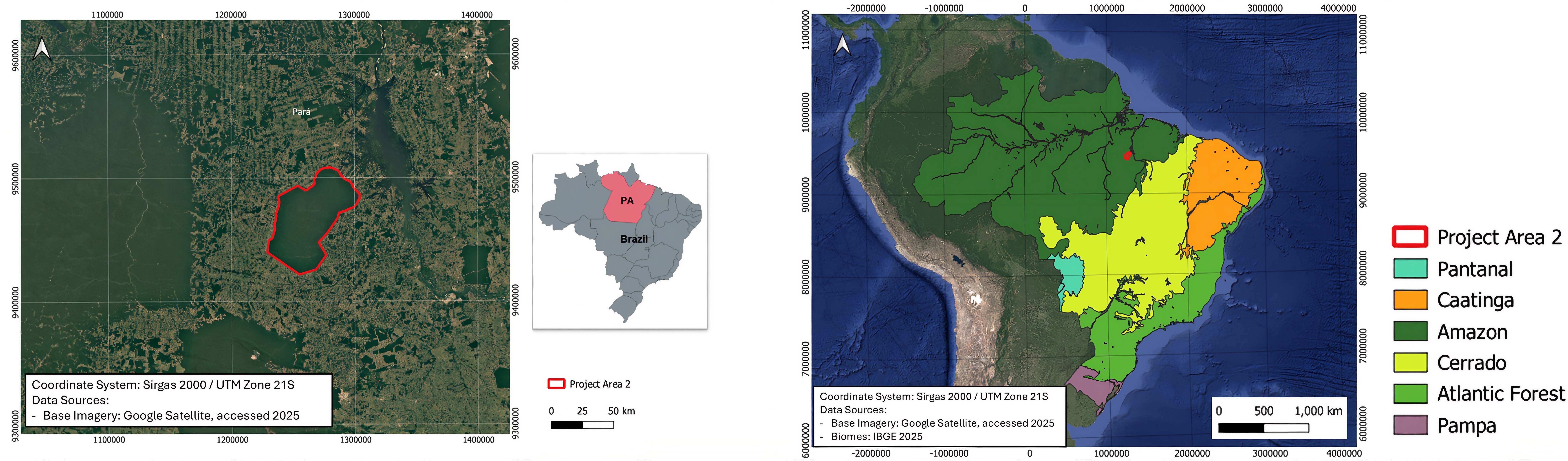
Figure 4. Location of case study 2, Parakanã Indigenous Territory.
RESULTS
Application of the RACZ framework to the two similar-sized while contrasting landscapes produced distinct spatial extents and configurations of degradation risk [Figure 5], indicating differences in surrounding deforestation pressure and landscape structure. The RACZ areas ranges from 1,150 ha in the low-pressure landscape to 337,985 ha in the high-pressure one, confirming the sensitivity of the exponential decay model to fragment geometry and external pressure [Table 1].
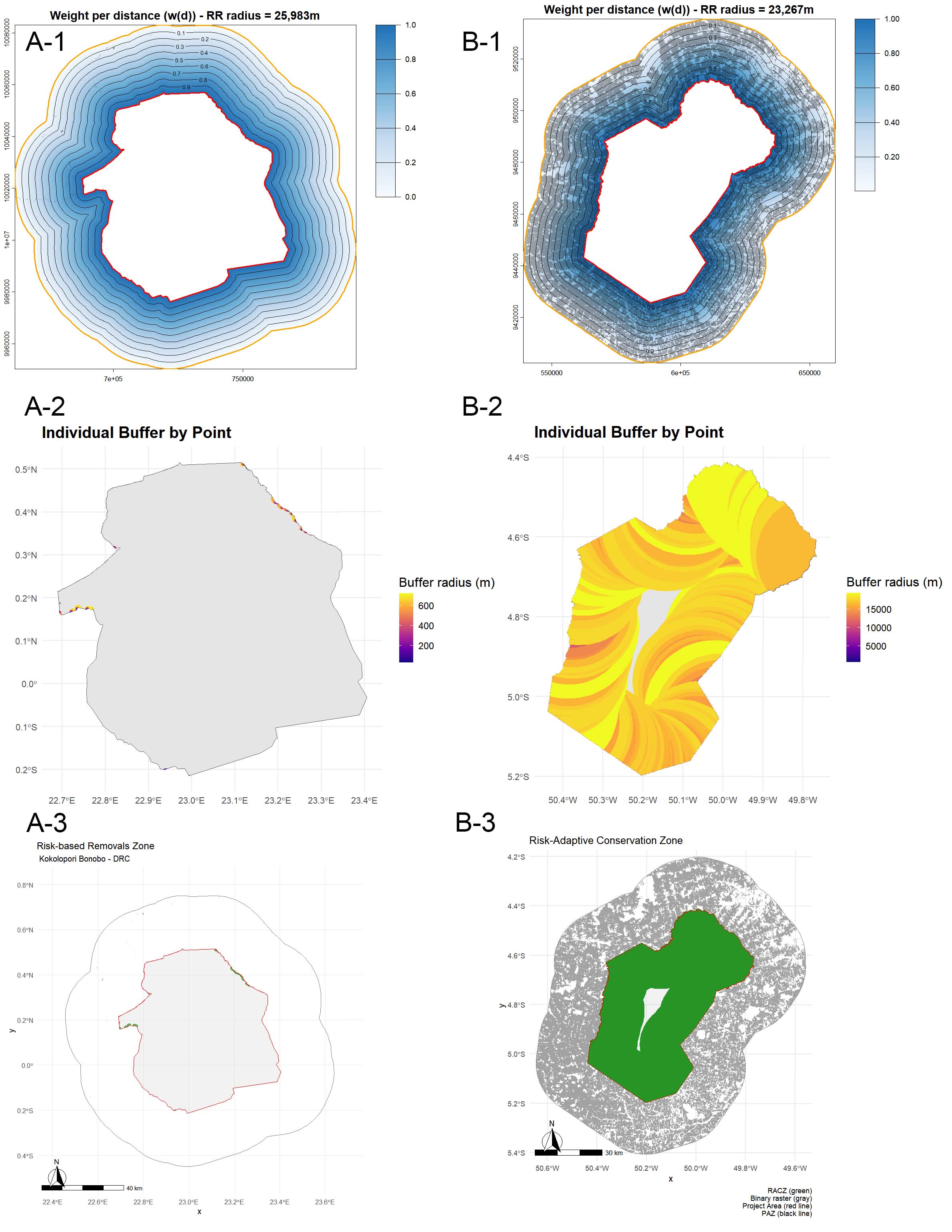
Figure 5. RACZ (A-3, B-3) derived from spatially variable buffer radius (A-2, B-2) and raster of weight per distance (A-1, B-1) in low- and high- pressure landscapes. In A-1 and B-1, Grey patches represent the pixels of deforestation. The contour lines represent intervals of the decay function, with values decreasing from 1.0 at the project edge (red polygon) to 0.0 at the maximum influence distance. Darker blue areas indicate regions of stronger potential influence from external anthropogenic pressure, while lighter tones represent rapidly decreasing influence with increasing distance.
Test results for RACZ model application in landscapes with contrasting external pressure and internal resilience
| Case study ID | Name | Country | Area (ha) | RRradius (m) | PLw | α (m) | CI | k | β (m-1) | RACZ (ha) |
| 1 | Kokolopori Bonobo Natural Reserve | Democratic Republic of the Congo | 424,200 | 25,983 | 0.0008 | 719 | 0.61 | 0.0071 | 0.0043 | 1,150 |
| 2 | Indigenous Territory Parakanã | Brazil | 340,100 | 23,267 | 0.83 | 19,407 | 0.49 | 0.0055 | 0.0027 | 337,985 |
Low-pressure landscape
In Kokolopori Bonobo Natural Reserve, Democratic Republic of the Congo, deforestation within the RR was minimal [Figure 5A-1]. The weighted landscape class proportion (PLw) was 0.0008, indicating that less than 0.1% of the surrounding areas contribute to deforestation on the project boundary. Such an extremely low value reflects the scarcity of consolidated deforestation around the site and confirms that the project area is embedded in a largely intact forest matrix. Consequently, the correction factor applied to the initial α parameter, derived from PLw, was also extremely small, resulting in a maximum ecological influence distance (α) of only 719 m. This short maximum reach already signals that anthropogenic effects do not propagate far into the landscape, consistent with an environment under minimal external disturbance.
The structural characteristics of the project area reinforce this pattern of low vulnerability. The site encompasses more than 400,000 hectares and exhibits a relatively compact geometry (CI = 0.61), resulting in a relatively high decay rate (β = 0.0043m-1). Therefore, whatever disturbance pressure exists diminishes rapidly with increasing distance from deforested pixels. When this β value is combined with the α parameter, the resulting exponential decay function produces a RACZ of only 1,150 hectares, around 0.27% of the entire area. Spatially, this RACZ is concentrated in narrow strips adjacent to isolated deforestation points and does not extend far into the forest interior [Figure 5A-2 and A-3].
High-pressure landscape
In contrast, the indigenous land Parakanã exhibited extensive surrounding deforestation [Figure 5B-1]. The resulting PLw value of 0.83 indicates that more than 80% of the surrounding landscape contributes directly to deforestation-driven pressure on the project boundary. This level of exposure is characteristic of frontier contexts where deforestation is widespread, spatially aggregated, and strongly connected. Consequently, the correction factor applied to the initial α parameter was extremely high, producing a maximum external influence distance (α) of 19,407 m.
The structural characteristics of the project area further modulate this spatial influence. Despite encompassing over 340,000 hectares, the site exhibits a shape factor of 0.49, reflecting a moderately irregular geometry with a relatively high perimeter-to-area ratio. Such configurations reduce the stability of interior habitats by increasing the proportion of forest areas exposed to edge influence. Under these conditions, the model estimated a decay rate of β = 0.0027 m-1, which corresponds to a slower decline of disturbance intensity, i.e., higher external influence penetration, relative to the very large α. The result of applying the model to each point on the area's edge is shown in Figure 5B-2. The various overlapping buffers are merged and inserted into the area to generate the RACZ [Figure 5B-3]. When combined in the exponential decay formulation, the large α and relatively lower β produced a RACZ of 337,985 hectares [Figure 5B-2 and B-3], extending across most of the project area.
This expansive RACZ reflects the ecological reality of a landscape under intense anthropogenic pressure. Disturbance does not dissipate quickly and edge effects penetrate deeply into forest interiors due to both strong external forcing and structural fragmentation. The resulting pattern demonstrates how the RACZ framework responds sensitively to the joint effects of pressure and susceptibility, capturing a broad spatial footprint of vulnerability in contexts where degradation is both pervasive and spatially far-reaching.
DISCUSSION
The two case studies demonstrate how degradation risk emerges from the complex interaction between external anthropogenic pressure and internal structural resistance, reinforcing the need for spatially adaptive approaches in conservation planning and carbon-accounting methodologies. In low-pressure landscapes, sparse surrounding deforestation and largely intact structure produced higher β values, reflecting rapid attenuation of disturbance signals and resulting in narrow RACZ bands around forest edges. Conversely, in high-pressure frontier regions dominated by fragmentation and repeated disturbances, lower β values result in slow decay rates and extensive RACZ footprints, capturing the deeper penetration of spatially contagious degradation processes. Together, these outcomes demonstrate the RACZ model's capacity to distinguish structurally stable forests from landscapes subject to pervasive, spatially contagious degradation.
These contrasting patterns are aligned with long-standing expectations in landscape ecology. Fragments differ profoundly in their susceptibility to external pressures based on their size and shape[26,27]. Large, intact fragments maintain extensive core habitat and internal microclimatic stability, buffering external influences and producing steep, short-range degradation gradients. In contrast, small or irregular fragments exhibit disproportionately large perimeter-to-area ratios, increasing their exposure to temperature shifts, desiccation, wind turbulence, treefall rates, invasive species, and fire - leading to slower attenuation of edge effects and higher vulnerability to degradation[19,48]. The RACZ model operationalizes these mechanisms mathematically through the interaction of α and β:α describes the maximum spatial envelope in which risk might propagate, while β quantifies the structural resistance governing the rate of decay. As shown in our results, these parameters adjust intuitively across contrasting landscapes, emerging as functional descriptors of well-established ecological principles.
Recent empirical studies[14,49] show fragmentation-driven degradation represents a large and persistent carbon loss that is often comparable to, or exceeds, emissions from deforestation itself, providing strong support for our conceptual foundation. For example, persistent collapse of edge biomass in the Amazon between 2001 and 2015 amounted to 947 Tg C—nearly one-third of the carbon emitted through deforestation during the same period[14]. This indicates that fragmentation-driven degradation is a large and persistent carbon flux, often invisible to deforestation-only accounting frameworks. Complementing this Amazonian evidence, observations using GEDI LiDAR showed that canopy height and structural deficits extend 1-1.5 km, and up to 7 km in repeatedly disturbed tropical forests[49]. In our model, however, the parameter α is not the penetration depth of edge effects in the same sense as that study. Instead, α defines the maximum range over which degradation risk is allowed to be non-zero, after which the function is truncated to zero. The effective “depth” of the gradient inside that range is governed by β. Crucially, the thresholds used in Bourgoin et al.’s study[49] (95% structural recovery) map conceptually onto the β-derived decay distances in the RACZ model (e.g., distances at which R(d) declines to 1%-5% of edge influence), suggesting that the model’s decay function captures the same underlying ecological gradients observed across global tropical forests.
Growing evidence further reinforces the generality of this edge-driven deforestation pattern. Edge forests have been shown to undergo chronic structural degradation, becoming more vulnerable to fire, drought, and other disturbances than intact interiors[50]. A global synthesis[12] found that negative edge effects on above-ground biomass occur in 97% of the world’s forests, with average biomass deficits of ~16% near edges. A recent study further adds that small patch sizes and irregular geometries dramatically exacerbate biomass loss, showing how structural vulnerability accelerates forest degradation in highly fragmented landscapes[51].
Collectively, these empirical studies converge on a fundamental pattern: degradation is a spatially extensive, structurally mediated, and pressure-dependent process, rather than a localized or binary phenomenon (e.g., arbitrarily defined edge strips). The mechanisms they document—microclimatic changes, shifts in species interactions, increased tree mortality, fire susceptibility, and biomass decline—behave like diffusion processes traveling from disturbance sources into forest interiors. This is directly compatible with the exponential decay kernel adopted in RACZ, which is grounded in mathematical ecology and diffusion theory[35,42]. Through the α-β decomposition, RACZ captures both: (i) the potential extent of influence (α), reflecting the cumulative burden of external anthropogenic forces; and (ii) the resistance-based attenuation (β), reflecting structural susceptibility. In this sense, RACZ not only mirrors but formalizes and quantifies the ecological mechanisms that have been described qualitatively for decades.
The integration of external pressure and internal susceptibility is particularly relevant for carbon crediting, where traditional methodologies assume that carbon benefits derive solely from the avoidance of deforestation. These approaches neglect the large and growing body of evidence showing that intact forests adjacent to deforestation edges experience significant carbon losses via degradation. By restricting crediting to areas within the RACZ envelope—that is, where degradation risk is empirically and theoretically supported—the model improves the environmental integrity of carbon credits. It prevents over-crediting in low-pressure landscapes where risk is minimal and appropriately recognizes larger vulnerable areas in highly pressured, fragmented forests. In doing so, RACZ aligns carbon-accounting practices with contemporary scientific understanding of forest degradation, promoting transparency, defensibility, and ecological realism.
Implications for the NbS market and the integrity of carbon credits
The RACZ framework should not be understood as a methodological complement to existing ICVCM-approved REDD+ standards, but rather as a distinct and additional scope within nature-based solutions. REDD+ methodologies estimate avoided emissions by projecting future deforestation and quantifying the carbon losses that would occur in the absence of the project. By contrast, RACZ does not model deforestation trajectories; instead, it delineates the spatial extent of forest area that is vulnerable to degradation driven by proximity to anthropogenic land uses.
Whereas REDD+ methodologies model the risk of forest loss using distance to remaining forest as a predictor—consistent with its objective of forecasting where new clearing might occur—the RACZ model uses distance to deforestation to represent how already-established edges propagate structural and functional degradation into standing forests. This distinction aligns directly with empirical evidence, showing that edge-driven degradation reduces biomass, ecosystem function, biodiversity, and growth rates, even in forests that remain nominally intact.
In this sense, RACZ introduces a new conceptual scope for nature-based climate solutions, designed to protect the ecological integrity and growth potential of vulnerable forest margins. Rather than extending or substituting existing REDD+ frameworks, RACZ expands the methodological landscape by formalizing the spatial component of degradation risk and enabling crediting approaches that reflect the well-documented influence of fragmentation and anthropogenic proximity on long-term forest carbon dynamics.
The following are the potential implications of the RACZ approach for conservation-based carbon removal credits and the main innovations of the methodology.
Risk-adaptiveness as a mechanism for improving crediting accuracy
The RACZ framework offers a pathway for substantially improving the environmental integrity of carbon crediting by embedding ecological risk directly into the spatial definition of creditable areas. Current nature-based methodologies, particularly those relying on avoided deforestation, typically delineate project boundaries using projected deforestation risk or administrative units, implicitly assuming that vulnerability is uniform across landscapes that are, in reality, highly heterogeneous[5,52]. Such assumptions can lead to crediting forest areas that face little or no disturbance pressure, thereby weakening additionality and overstating climate benefits.
By contrast, RACZ introduces risk-adaptiveness as a core design principle. By integrating external anthropogenic pressure (operationalized as distance to deforestation) with internal ecological susceptibility (derived from fragment size, shape, and structural configuration), the model identifies the portions of a project area where degradation is most likely to occur. This ensures that crediting zones are geographically restricted to areas with demonstrable, ecologically justified vulnerability, rather than areas selected through uniform or administratively convenient rules.
In doing so, RACZ improves crediting accuracy by aligning carbon benefits with actual landscape processes, reducing the risk of over-crediting, and increasing transparency for both project developers and standard-setting bodies. The result is a crediting framework that is more scientifically defensible, more consistent with contemporary understanding of forest degradation dynamics, and better suited to support high-integrity nature-based climate solutions. Therefore, RACZ provides a more defensible and scientifically coherent basis for avoiding over-crediting while strengthening environmental integrity across carbon portfolios.
Supporting dynamic, evidence-based buffering
The proposed approach provides a scientifically grounded delineation of the areas that crediting areas reflect actual zones of vulnerability. By deriving spatial risk directly from the α-β parameterization, RACZ translates decades of empirical knowledge on distance-decay processes, landscape ecology, and structural susceptibility[20,23,26,33,50,53] into an operational framework.
This evidence-based approach has direct implications for assessments of project performance. Because α captures the external pressure envelope and β encodes internal structural resistance, RACZ identifies zones where biomass, canopy structure, and ecological function are most vulnerable to degradation, areas that traditional deforestation-only baselines fail to recognize[14,45]. In doing so, RACZ enhances not only project-level accuracy but also portfolio-level conservativeness, an increasingly important criterion in international carbon standards aiming to improve environmental integrity.
Finally, the RACZ framework also strengthens conservation practice by identifying where forests are most vulnerable to edge-driven degradation, enabling more targeted deployment of restoration, fire prevention, and connectivity interventions. By operationalizing these insights into a practical spatial product, RACZ strengthens the capacity of conservation programs to anticipate degradation before it becomes irreversible, ultimately improving the long-term resilience of forest landscapes.
Limitations and future work
Although the RACZ framework provides a mechanistic, ecologically grounded approach for delineating degradation-risk-adaptive conservation zones, several important limitations should be acknowledged.
First, the current approach infers spatial vulnerability from structural and contextual predictors—distance to deforestation, landscape configuration, and pressure indices—without yet incorporating temporal validation of degradation processes. While extensive literature supports the assumption that RACZ-identified areas are more susceptible to biomass loss, microclimatic alteration, and biodiversity decline, the model has not been explicitly tested using time-series observations of canopy height, above-ground biomass, spectral degradation indices, or species-level responses within RACZ zones. Longitudinal validation using LiDAR, radar backscatter, repeat optical imagery, or ecological plot networks will be essential to confirm whether RACZ-delineated areas indeed undergo accelerated structural or functional degradation, and to refine the decay parameters accordingly.
Second, some components of the model, particularly the area factor, shape-based adjustments, and landscape-specific decay rates, were calibrated using a combination of ecological theory and generalized empirical regularities. While these formulations capture broad ecological patterns, they may not fully represent biome-specific or region-specific dynamics. Forests differ widely in their sensitivity to fragmentation. For example, humid tropical forests often show deep structural degradation gradients, whereas dry forests, savannas, and temperate systems may exhibit different decay rates or disturbance propagation pathways. Future work should therefore explore biome-specific parameterizations, including alternative α and β distributions, distinct formulations for shape and area-derived susceptibility, and possibly additional modifiers such as climatic seasonality, fire regimes, hydrological connectivity, or species composition.
A related limitation lies in the structure of the decay function. The model assumes a simple exponential model, which is consistent with diffusion-based ecological theory but may not capture multimodal or threshold-driven behavior observed in some ecosystems, such as abrupt biomass collapse following fire incursion, nonlinear feedbacks from edge-driven mortality, or spatial contagion reinforced by human activities. Likewise, the assumption that the nearest deforested pixel is the dominant source of degradation pressure may underestimate risks in landscapes with multiple interacting disturbances dynamically over time, such as selective logging, chronic understory fire, or edge-induced drought stress.
Revalidation of the model with updates of the RACZ area’s delineation, incorporating multi-source disturbance layers and probabilistic representations of disturbance interactions, may help refine RACZ estimates. The framework assumes that deforestation is the primary and spatially continuous driver of disturbance, such that distance to the nearest deforestation provides a proxy for degradation risk. This assumption may be less appropriate in landscapes dominated by multi-source or strongly directional disturbances, where cumulative or anisotropic effects are not explicitly captured. Integrating multi-source disturbance into the model, as well as with predictive models of land-use change, fire spread, or road expansion could strengthen its utility for long-term conservation planning and dynamic carbon-crediting.
At a broader level, an important limitation is the dependence on the quality of deforestation and land-cover data. Spatial errors in deforestation detection, classification bias, or temporal inconsistencies may propagate uncertainty into the risk surface.
Future research should therefore focus on three key areas:
(1) Temporal validation, using independent multi-sensor datasets (GEDI, ICESat-2, Sentinel-1/2, Landsat harmonics) to test whether RACZ-designated zones systematically undergo greater biomass, canopy, or biodiversity loss.
(2) Biome and region-specific parameterization, ensuring that α, β, and the area-factor spline reflect structural and ecological realities of distinct forest types.
(3) Model expansion and integration, incorporating additional disturbance pathways, alternative decay functions, and links to predictive spatial models.
Despite these limitations, the RACZ framework represents an important step toward more ecologically realistic, empirically grounded, and risk-adaptive zoning for carbon crediting.
CONCLUSION
This study presents a spatially explicit framework for modeling degradation risk based on distance to deforestation and landscape structure. The RACZ model formalizes the relationship between anthropogenic pressure and forest condition through a distance-decay function, enabling the delineation of conservation areas grounded in ecological processes.
The framework was shown to be consistent across contrasting landscape contexts, demonstrating its ability to represent spatial variability in degradation risk and to translate ecological principles into an operational tool for conservation and carbon accounting.
By integrating spatial dynamics and ecological structure into a unified formulation, the RACZ model provides a transparent and adaptable approach for identifying areas of vulnerability. Future work should focus on expanding the framework. Continued refinement and validation will enhance its robustness and ensure that it remains aligned with contemporary scientific understanding of forest degradation dynamics.
DECLARATIONS
Acknowledgments
We’d like to thank Aurélien Vivancos and Vanessa Fuentes Suguiyama in C3 Ambiental for their comments on the paper.
Authors’ contributions
Development of concept and model, data analysis: Corsini, C.
Writing-original draft, editing & supervision: Corsini, C.; Chaib, J.; Wang, H.
Edited and revised the manuscript: Corsini, C.; Chaib, J.; Davies, M.; Centeno, D.; Feldmann, R.; Wang, H.
Availability of data and materials
The datasets used and/or analyzed in the current study are available from the corresponding author upon reasonable request.
AI and AI-assisted tools statement
During the preparation of this manuscript, the AI tool ChatGPT (version 5.3, released 2026-03-03) was used solely for language editing and for the creation of the graphical abstract. The tool did not influence the study design, data collection, analysis, interpretation, or the scientific content of the work. All authors take full responsibility for the accuracy, integrity, and final content of the manuscript.
Financial support and sponsorship
None.
Conflicts of interest
All authors declared that there are no conflicts of interest.
Ethical approval and consent to participate
Not applicable.
Consent for publication
Not applicable.
Copyright
© The Author(s) 2026.
REFERENCES
1. Griscom, B. W.; Adams, J.; Ellis, P. W.; et al. Natural climate solutions. Proc. Natl. Acad. Sci. USA. 2017, 114, 11645-50.
2. Angelsen, A.; Martius, C.; De Sy, V.; Duchelle, A.; Larson, A.; Thuy, P. Transforming REDD+: lessons and new directions. Center for International Forestry Research (CIFOR); 2018.
3. Delacote, P.; Chabé-Ferret, S.; Creti, A.; et al. Restoring credibility in carbon offsets through systematic ex post evaluation. Nat. Sustain. 2025, 8, 733-40.
4. West, T. A. P.; Alford-Jones, K.; Delacote, P.; et al. Demystifying the romanticized narratives about carbon credits from voluntary forest conservation. Global. Chang. Biol. 2025, 31, e70527.
5. West, T. A. P.; Börner, J.; Sills, E. O.; Kontoleon, A. Overstated carbon emission reductions from voluntary REDD+ projects in the Brazilian Amazon. Proc. Natl. Acad. Sci. USA. 2020, 117, 24188-94.
6. Probst, B. S.; Toetzke, M.; Kontoleon, A.; et al. Systematic assessment of the achieved emission reductions of carbon crediting projects. Nat. Commun. 2024, 15, 9562.
7. Ecosystem Marketplace. 2023. Available from: https://www.ecosystemmarketplace.com/publications/state-of-the-voluntary-carbon-market-report-2023/ [Last accessed on 22 Jun 2026].
8. Fastmarkets. Carbon credit demand plateaued in 2025 as buyers sorted by quality, compliance and durability. 2025. Available from: https://www.fastmarkets.com/insights/carbon-credit-demand-plateaued-in-2025-as-buyers-sorted-by-quality-compliance-and-durability/ [Last accessed on 22 Jun 2026].
9. West, T. A.; Bomfim, B.; Haya, B. K. Methodological issues with deforestation baselines compromise the integrity of carbon offsets from REDD+. Global. Environ. Chang. 2024, 87, 102863.
10. Tang, Y.; Yang, C.; Wu, H.; et al. Tropical forest carbon offsets deliver partial gains amid persistent over-crediting. Science 2025, 390, 182-7.
11. Swinfield, T.; Toye Scott, E. Scientific credibility for high-integrity voluntary carbon markets. Earth. Environ. Sci. 2025.
12. Yang, G.; Crowther, T. W.; Lauber, T.; Zohner, C. M.; Smith, G. R. A globally consistent negative effect of edge on aboveground forest biomass. Nat. Ecol. Evol. 2025, 9, 2036-45.
13. Aguilar-Amuchastegui, N.; Riveros, J. C.; Forrest, J. L. Identifying areas of deforestation risk for REDD+ using a species modeling tool. Carbon. Balance. Manag. 2014, 9, 10.
14. Silva Junior, C. H. L.; Aragão, L. E. O. C.; Anderson, L. O.; et al. Persistent collapse of biomass in Amazonian forest edges following deforestation leads to unaccounted carbon losses. Sci. Adv. 2020, 6, eaaz8360.
15. Qie, L.; Lewis, S. L.; Sullivan, M. J. P.; et al. Long-term carbon sink in Borneo’s forests halted by drought and vulnerable to edge effects. Nat. Commun. 2017, 8, 1966.
16. Matricardi, E. A. T.; Skole, D. L.; Costa, O. B.; Pedlowski, M. A.; Samek, J. H.; Miguel, E. P. Long-term forest degradation surpasses deforestation in the Brazilian Amazon. Science 2020, 369, 1378-82.
17. Assis, T. O.; Aguiar, A. P. D.; Von Randow, C.; Nobre, C. A. Projections of future forest degradation and CO2 emissions for the Brazilian Amazon. Sci. Adv. 2022, 8, eabj3309.
18. Berenguer, E.; Armenteras, D.; Lees, A. C.; et al. Drivers and ecological impacts of deforestation and forest degradation in the Amazon. Acta. Amaz. 2024, 54, e54es22342.
19. Broadbent, E. N.; Asner, G. P.; Keller, M.; Knapp, D. E.; Oliveira, P. J.; Silva, J. N. Forest fragmentation and edge effects from deforestation and selective logging in the Brazilian Amazon. Biol. Conserv. 2008, 141, 1745-57.
20. Haddad, N. M.; Brudvig, L. A.; Clobert, J.; et al. Habitat fragmentation and its lasting impact on Earth’s ecosystems. Sci. Adv. 2015, 1, e1500052.
21. Lapola, D. M.; Pinho, P.; Barlow, J.; et al. The drivers and impacts of Amazon forest degradation. Science 2023, 379, eabp8622.
22. Laurance, W. Hyper-disturbed parks: edge effects and the ecology of isolated reserves in tropical Australia. In Tropical Forest Remnants: Ecology, Management, and Conservation of Fragmented Communities; University of Chicago Press, 1997; pp. 71-84. Available from: https://www.researchgate.net/publication/313644549_Hyper-disturbed_parks_Edge_effects_and_the_ecology_of_isolated_reserves_in_tropical_Australia [Last accessed on 26 Jun 2026].
23. Laurance, W. F.; Camargo, J. L.; Luizão, R. C.; et al. The fate of Amazonian forest fragments: a 32-year investigation. Biol. Conserv. 2011, 144, 56-67.
24. Chaplin-Kramer, R.; Ramler, I.; Sharp, R.; et al. Degradation in carbon stocks near tropical forest edges. Nat. Commun. 2015, 6, 10158.
25. Esquivel-Muelbert, A.; Baker, T. R.; Dexter, K. G.; et al. Compositional response of Amazon forests to climate change. Global. Chang. Biol. 2018, 25, 39-56.
26. Murcia, C. Edge effects in fragmented forests: implications for conservation. Trends. Ecol. Evol. 1995, 10, 58-62.
27. Harper, K. A.; Macdonald, S. E.; Burton, P. J.; et al. Edge influence on forest structure and composition in fragmented landscapes. Conserv. Biol. 2005, 19, 768-82.
28. Berenguer, E.; Ferreira, J.; Gardner, T. A.; et al. A large-scale field assessment of carbon stocks in human-modified tropical forests. Global. Chang. Biol. 2014, 20, 3713-26.
29. Taubert, F.; Fischer, R.; Groeneveld, J.; et al. Global patterns of tropical forest fragmentation. Nature 2018, 554, 519-22.
30. Turner, M. G.; Gardner, R. H. Landscape ecology in theory and practice: pattern and process. New York, NY: Springer; 2015.
31. Mcgarigal, K.; Cushman, S. A. Comparative evaluation of experimental approaches to the study of habitat fragmentation effects. Ecol. Appl. 2002, 12, 335.
32. Fletcher, R. J. Multiple edge effects and their implications in fragmented landscapes. J. Anim. Ecol. 2005, 74, 342-52.
33. Ewers, R. M.; Didham, R. K. Confounding factors in the detection of species responses to habitat fragmentation. Biol. Rev. 2005, 81, 117.
34. Su, Y.; Zhang, C.; Cescatti, A.; et al. Pervasive but biome-dependent relationship between fragmentation and resilience in forests. Nat. Ecol. Evol. 2025, 9, 1670-84.
35. Okubo, A.; Levin, S. A. The basics of diffusion. In: Diffusion and ecological problems: modern perspectives. New York, NY: Springer New York; 2001. pp. 10-30.
37. Laurance, W. F.; Ferreira, L. V.; Rankin-de Merona, J. M.; Laurance, S. G. Rain forest fragmentation and the dynamics of amazonian tree communities. Ecology 1998, 79, 2032.
38. Fortin, M.; Dale, M. R. T. Spatial analysis: a guide for ecologists. Cambridge University Press; 2009.
39. Forman, R. T. T.; Wilson, E. O. Land mosaics: the ecology of landscapes and regions. Cambridge University Press; 2018.
40. Hansen, M. C.; Wang, L.; Song, X.; et al. The fate of tropical forest fragments. Sci. Adv. 2020, 6, eaax8574.
41. Haines-Young, R.; Chopping, M. Quantifying landscape structure: a review of landscape indices and their application to forested landscapes. Prog. Phys. Geogr. Earth. Environ. 1996, 20, 418-45.
43. Project MapBiomas. Collection 10 of the annual series of land use and land cover in Brazil. Available from: https://brasil.mapbiomas.org/colecoes-mapbiomas/ [Last accessed on 22 Jun 2026].
44. Souza, C. M.; Shimbo, J. Z.; Rosa, M. R.; et al. Reconstructing three decades of land use and land cover changes in brazilian biomes with landsat archive and earth engine. Remote. Sens. 2020, 12, 2735.
45. McGarigal, K.; Cushman, S. A.; Ene, E. FRAGSTATS v4: spatial pattern analysis program for categorical and continuous maps; University of Massachusetts: Amherst, MA, 2012. Available from: http://www.umass.edu/landeco/research/fragstats/fragstats.html [Last accessed on 22 Jun 2026].
46. Fritsch, F. N.; Carlson, R. E. Monotone piecewise cubic interpolation. SIAM. J. Numer. Anal. 1980, 17, 238-46.
47. Aràndiga, F.; Baeza, A.; Yáñez, D. F. Monotone cubic spline interpolation for functions with a strong gradient. Appl. Numer. Math. 2022, 172, 591-607.
48. Brinck, K.; Fischer, R.; Groeneveld, J.; et al. High resolution analysis of tropical forest fragmentation and its impact on the global carbon cycle. Nat. Commun. 2017, 8, 14855.
49. Bourgoin, C.; Ceccherini, G.; Girardello, M.; et al. Human degradation of tropical moist forests is greater than previously estimated. Nature 2024, 631, 570-6.
50. Sun, M.; Li, W.; Zhu, L.; et al. Degradation in edge forests caused by forest fragmentation. Carbon. Res. 2025, 4, 38.
51. Sgarlata, G. M.; Maié, T.; De Zoeten, T.; Salmona, J.; Rasteiro, R.; Chikhi, L. The effect of habitat loss and fragmentation on isolation by distance and divergence. Proc. Natl. Acad. Sci. USA. 2025, 122, e2410951122.
52. Badgley, G.; Freeman, J.; Hamman, J. J.; et al. Systematic over-crediting in California's forest carbon offsets program. Global. Chang. Biol. 2021, 28, 1433-45.
Cite This Article
How to Cite
Download Citation
Export Citation File:
Type of Import
Tips on Downloading Citation
Citation Manager File Format
Type of Import
Direct Import: When the Direct Import option is selected (the default state), a dialogue box will give you the option to Save or Open the downloaded citation data. Choosing Open will either launch your citation manager or give you a choice of applications with which to use the metadata. The Save option saves the file locally for later use.
Indirect Import: When the Indirect Import option is selected, the metadata is displayed and may be copied and pasted as needed.
About This Article
Special Topic
Copyright

Data & Comments
Data
0


Comments
Comments must be written in English. Spam, offensive content, impersonation, and private information will not be permitted. If any comment is reported and identified as inappropriate content by OAE staff, the comment will be removed without notice. If you have any queries or need any help, please contact us at [email protected].