

A spatial multi-scale reservoir computing framework for power flow analysis in power grids
 0
0 Abstract
With the ongoing evolution of modern power grids, power flow calculation, which is the cornerstone of power system analysis and operation, has become increasingly complex. While promising, existing data-driven methods struggle with key challenges: poor generalization in data-scarce scenarios, efficiency bottlenecks when integrating physical laws, and a failure to capture higher-order interactions within the grid. To address these challenges, this paper proposes a Spatial Multi-scale Reservoir Computing framework that seamlessly incorporates functional matrix and physical information to solve power flow calculation. The framework utilizes parallel readout layer parameters to construct the functional matrix and integrates physical information to create a multi-scale information processing mechanism and readout constraints. By improving the reservoir computing model, the framework also combines the reservoir paradigm with the inherent physical characteristics of power grids while maintaining computational efficiency. Experimental results demonstrate that the presented framework achieves exceptional performance across various IEEE bus systems, showcasing superior generalization in data-scarce scenarios, as well as improvement in computational speed, prediction accuracy, and robustness, while ensuring the feasibility of the output results.
Keywords
1. INTRODUCTION
With the evolution of the economy and the profound changes in the energy generation and consumption, the scale and structure of modern power grids have become increasingly diverse, and the operational characteristics of the system have become more complex, while also facing greater uncertainties[1,2]. Power flow calculation, as a fundamental component of power system analysis and operation, is also a prerequisite for advanced applications such as stability analysis and optimal dispatching, playing a critical role in ensuring the safe and economical operation of power grids[3,4]. However, in the face of highly nonlinear modern power grids, some traditional numerical methods or heuristic methods often have problems such as non-convergence or low computational efficiency when solving power flow, which make them face considerable challenges in computation and decision support[5,6].
To address these challenges, researchers have increasingly focused on the application of artificial intelligence, especially machine learning and deep learning, in power system analysis and power flow calculations[7,8,9]. These methods have shown significant potential to improve computational speed and handle complex nonlinear relationships. Some of the early data-driven models faced challenges such as limited generalization, inadequate consideration of underlying physical mechanisms, and insufficient accounting for the local-global topological interdependence they entail, especially when applied to highly nonlinear and dynamically evolving complex systems such as power grids[10,11]. Later, with the rise of the graph neural and physics-informed approaches, researchers have sought to integrate the physical mechanisms or topology of power grids with data-driven models[12], but these also introduce the challenge of balancing model complexity and computational efficiency. Moreover, due to the complex and special nature of the electrical environment, models sometimes also face challenges in robustness and data scarcity[13].
Recently, a computational framework known as reservoir computing (RC) has attracted significant attention in the study of complex systems[14,15]. This paradigm circumvents the need for backpropagating error signals, thereby enhancing both robustness and training efficiency. Owing to the high-dimensional and nonlinear dynamics of the reservoir, RC can effectively extract rich and distinguishable dynamic features from the system, even with limited historical data[16]. The RC paradigm has seen some exploratory applications in power systems[17], which are typical complex dynamical systems, but RC′s use for analyzing power flow remains quite limited.
Motivated by these challenges, this paper proposes the Spatial Multi-scale Reservoir Computing (SMsRC) framework to improve standard RC for power flow calculation. It has three key innovations: first, a functional matrix is introduced to deterministically encode each bus′s role, overcoming the limitations of random input weights; second, a spatial multi-scale analysis captures complex dependencies from higher-order, non-local neighbors; third, physical information is incorporated as a constraint on the readout layer to ensure outputs obey fundamental power flow laws. The main contributions are summarized as follows:
● Considering the advantages of the RC in efficiency and stability, especially for limited-data scenarios, a novel spatial multi-scale reservoir model is proposed and integrated with physical mechanisms to construct a power flow solving framework named SMsRC.
● Three core innovations are introduced in the SMsRC framework. First, a functional matrix replaces random input weights to encode each bus′s role, providing data-driven priors. Second, a multi-scale spatial structure captures complex dependencies from higher-order and non-local neighbors for a fuller system representation. Third, physical constraints are applied directly to the RC readout layer, ensuring outputs follow basic power flow laws while maintaining efficiency.
● The performance of the SMsRC framework is validated in solving the power flow across different IEEE bus systems. Compared with other data-driven methods, particularly in the few-shot scenario, the SMsRC demonstrates stronger generalizability, achieving faster training and prediction while ensuring accuracy. Meanwhile, SMsRC shows robustness for diverse power grid scenarios.
The remainder of this article is organized as follows. Section 2 reviews the related work. Section 3 introduces the preliminary concepts and problem definitions. Section 4 outlines the proposed SMsRC framework in detail. Section 5 presents the experimental setup along with the results, and finally, Section 6 concludes the paper with discussions.
2. RELATED WORK
Current methods for power flow calculation fall into three categories: traditional numerical methods, heuristic search methods, and data-driven methods.
2.1. Traditional numerical methods
Numerical methods model power grid operational constraints and objective functions as mathematical equations, deriving optimal flow solutions via numerical iterations[18]. Examples include the Newton-Raphson, Gauss-Seidel, and fast-decoupled power flow methods, etc.[19]. Additionally, to improve the convergence, Niu et al.[20] designed methods based on Taylor series expansion and improved Newton methods. Montoya et al.[21] proposed backward/forward sweep methods based on graph theory and improved algorithms based on rectangular coordinates, improving calculation speed and accuracy under specific conditions. Tang et al.[22] developed an Alternating Current optimal power flow calculation method based on the Quasi-Newton method. Despite these advancements, fundamentally, the non-linear and non-convex nature of the alternating current optimal power flow (AC-OPF) problem means they are computationally intensive, highly sensitive to initial values, and can easily get trapped in local optima, failing to find a global-like solution. This results in a lack of convergence and robustness, rendering them inadequate for the fast-timescale control of modern complex power systems. To address these convergence bottlenecks and sensitivity to initial conditions, heuristic search strategies were introduced to enhance global optimization capabilities.
2.2. Heuristic search methods
Researchers have also explored heuristic search methods for power flow calculation. These methods use novel search mechanisms to enhance exploration and exploitation, improving convergence and accuracy. They are typically used for multi-objective optimization problems difficult for traditional techniques[23,24]. The genetic algorithm was among the first heuristic methods applied to power flow[25]. Others include teaching–learning optimization, metaheuristic algorithms, and differential evolution algorithms[26,27], etc., all of which are used to solve optimal power flow problems involving both continuous and discrete control variables. However, these methods present trade-offs. While often more robust in avoiding poor local optima compared to numerical methods, they are notoriously computationally expensive and time-consuming[28]. Their performance is sensitive to the initial encoding of the problem and the specific design of the fitness function, including the penalty mechanisms for handling operational constraints. And they face persistent challenges in generalizing effectively to high-dimensional nonlinear systems. These computational bottlenecks have motivated the emergence of data-driven methods, which aim to learn complex mappings directly from historical data without explicit iterative optimization.
2.3. Data-driven methods
With the rapid advancement of deep learning technologies and the growing complexity of modern power grids, there has been increasing research interest in data-driven approaches. These methods are capable of automatically learning feature patterns directly from data, without the need for precise prior knowledge[29,30]. Currently, the models applied to power flow are primarily based on deep neural networks (DNNs) or graph neural networks (GNNs), as well as physics-informed neural networks expanded on this basis[31]. Hansen et al.[32] developed an end-to-end framework based on line GNNs to balance the power flow in energy grids. Lopez-Garciaet al.[3] developed a typed GNN with linear complexity that solves the power flow problem through an unsupervised method of minimizing the violation of physical laws. In addition, ensuring feasible solutions is crucial in power flow problems. Some studies verify or refine model outputs using additional optimizers or classifiers[33], while others enhance accuracy and feasibility by incorporating physical information[34]. However, these approaches often rely on complex penalty-based loss functions to address the limitations of general models such as DNNs or GNNs[35], which can increase computational cost, complicate gradient calculation, and sometimes lead to parameter sensitivity or unstable outputs. These observations motivate our proposed SMsRC framework that can organically integrate physical laws with efficient learning paradigms to simultaneously ensure computational speed and solution feasibility.
To highlight the research gap, Table 1 compares existing methods with the proposed SMsRC framework. SMsRC addresses previous limitations by integrating physical constraints and functional priors, balancing efficiency, generalization, and physical consistency.
Comparisons of characteristics and limitations among different power flow calculation methods
| Category | Representative methods | Characteristics & limitations (pain points) | Evolution & superiority of SMsRC |
| Traditional numerical methods (Rule-based) | Newton-Raphson, Gauss-Seidel, Fast-decoupled methods (e.g., [18,19,20]) | Char: Solves mathematical equations based on physical laws via iterations Limits: Computationally intensive; highly sensitive to initial values; prone to non-convergence in complex, non-convex AC-OPF problems. | SMsRC replaces the rigid iterative solving process with a learned non-linear mapping, avoiding non-convergence issues while maintaining physical feasibility through constrained readout layers |
| Heuristic search methods (Evolutionary) | Genetic Algorithm (GA), PSO, Differential Evolution (e.g., [25,26,27]) | Char: Global optimization mechanisms; effective for discrete variables Limits: Extremely computationally expensive and time-consuming; performance is sensitive to encoding and fitness function design | Leveraging the echo state property of Reservoir Computing (RC), SMsRC achieves extremely fast training and inference speeds, addressing the computational bottleneck of heuristic search methods |
| Existing data-driven methods (Machine learning) | DNN, GNN, PINN (e.g.,[32,3,31]) | Char: Fast inference; automatic feature extraction from data Limits: Poor generalization in data-scarce scenarios; often neglects high-order topological dependencies; struggles to strictly guarantee physical consistency (feasibility) | Addressing data-driven gaps: 1. Functional matrix: Replaces random weights to encode bus roles (Deterministic vs. Random) 2. Spatial multi-scale: Captures long-range/high-order dependencies often missed by standard GNNs 3. Physical constraints: Directly integrates power laws into the readout to ensure valid solutions |
| Proposed framework | SMsRC (This paper) | Char: A spatial multi-scale reservoir computing framework integrated with functional matrix and physical information | Synthesis: SMsRC combines the efficiency of RC with the rigour of physical laws. It demonstrates superior robustness and accuracy, especially in few-shot scenarios where pure data-driven methods fail |
3. PRELIMINARIES AND PROBLEM FORMULATION
To rigorously formulate the power flow solving problem addressed in this paper, this section introduces the theoretical and physical foundations alongside the mathematical definition. Specifically, Section 3.1 first outlines the basic principles of RC, which serves as the core computational engine of the proposed framework. Subsequently, Section 3.2 describes the physical characteristics and governing equations of the power flow in power grids, defining the key variables and node types. Finally, based on the computational paradigm introduced in Section 3.1 and the system variables defined in Section 3.2, Section 3.3 formally presents the mathematical formulation of the data-driven power flow calculation problem.
3.1. Reservoir computing (RC)
RC, as a machine learning paradigm that has gained attention in the field of complex systems in recent years, has its core idea in performing nonlinear transformations with the help of a randomly connected neural network (i.e., the reservoir), and then achieving the output of specific tasks by training the weights of the readout layer[36].
Echo State Network (ESN), as a prominent implementation of RC, features a basic architecture comprising three core parts: the input layer, the reservoir, and the readout layer. Operations related to these three parts mainly include initializing the input matrix
For the problem of the power flow calculation, which is a system of nonlinear equations, the training process of the ESN can be characterized using [38,39]:
where
3.2. Power flow
In power system operations, two primary power flow models are widely used: direct current optimal power flow (DC-OPF) and AC-OPF. Although the DC-OPF model is relatively simple to compute, its precision is compromised due to the variations in reactive power and voltage magnitude. In contrast, the AC-OPF model considers more comprehensive system characteristics, providing a more accurate description of the actual system′s operational state. Therefore, this study adopts AC-OPF as the foundational model.
Under steady-state conditions, buses in a power grid can be classified into three types: PQ buses, PV buses, and slack bus. Each type of bus is characterized by distinct known and unknown parameters. Specifically, PQ buses correspond to load nodes, with known active power
The AC-OPF problem seeks to minimize the operational cost of the system while adhering to various physical and operational constraints[40]:
where
3.3. Problem formulation
This study aims to develop a power flow solving framework based on the RC paradigm, integrating physical functional information of the power grid to enrich the priors. The problem can be formally defined as follows:
where
More specifically, each row of the input matrix
where
The structure of the output matrix
where
4. PROPOSED FRAMEWORK
While data-driven methods show promise for power flow calculations, they often struggle to balance computational efficiency with physical consistency, especially under data-scarce conditions. To bridge these gaps, this paper proposes the SMsRC framework, which customizes the RC paradigm by deeply integrating it with power grid physics. Distinct from generic data-driven models, SMsRC introduces three problem-oriented innovations: (1) a Functional Matrix replaces random initialization to explicitly encode the heterogeneous functional roles of grid buses; (2) a Spatial Multi-scale mechanism is constructed to capture both local and global topological dependencies essential for power flow distribution; and (3) Physical Constraints are enforced in the readout layer to ensure solution feasibility while retaining RC′s rapid training advantages, avoiding the instability of complex penalty-based loss functions.
The framework aims to learn the solution function
where
The schematic diagram of presented SMsRC framework is presented in Figure 1. To better illustrate, the IEEE14 bus system is considered, as shown in Figure 1(a). A set of driving data, consisting of the known variable values of each bus, together with a set of physical information
Figure 1. Schematic diagram of the power flow solving framework SMsRC. (a) Driving information and IEEE14 bus system configuration with known/unknown variables. (b) Parallel Echo State Network for initial state learning. (c) Extraction of functional vectors via parameter compression. (d) Identification of higher-order neighbors via node-pair prediction losses. (e) Architecture of the Spatial Multi-scale Reservoir Computing. (f) Physical constraint module for readout layer solving. (g) Final feasible power flow solution.
4.1. Parallel learning auxiliary information
This stage focuses on learning two types of essential auxiliary information for the model: functional feature vectors and higher-order neighbors. The process consists of three steps. First, a parallel ESN architecture is used to generate bus-specific prediction outputs. Second, the resulting parameters are compressed into functional vectors that characterize the unique functional role of each bus. Finally, prediction losses between bus pairs are analyzed to identify higher-order neighbors-buses that exert significant influence despite not being directly connected.
4.1.1. Generating bus-specific prediction outputs via ESNs
First, the conventional ESNs are employed, where each of the
The purpose here is to observe the global state from the perspective of a single local bus with a certain bias.
A set of readout layer weight matrices
Figure 2. Schematic diagram of functional localization. Visualization of the readout layer weights of the parallel reservoirs corresponding to buses 1, 2, 3, 8, 9, and 12 in the IEEE14 bus system. For this test case, the output dimension is 28, and the number of nodes in each reservoir is 56.
4.1.2. Constructing functional feature of each bus via compression operation
Based on above characteristics,
4.1.3. Identifying higher-order neighbors via prediction loss
To uncover deep relationships between different buses, that is, to determine the potential higher-order neighbor information for each bus, the BPLoss metric is introduced to evaluate the loss of each bus relative to others. Define
where
Based on the
4.2. Reconstructing input matrix and input information
This stage utilizes the two types of auxiliary information from the previous stage to construct two key components: the functional matrix
4.2.1. Constructing the functional matrix
The functional feature vectors
4.2.2. Constructing the spatial multi-scale information
Bus information is passed and aggregated based on the neighbor information of buses. However, since the types and attribute values of buses and their neighbors may differ, direct aggregation and summation could lead to inaccuracies or distortions in the information, potentially misleading the model. To address this, the equivalent conversion value based on physical mechanisms is incorporated to ensure physical consistency and validity during the passing process. First, an influence weight
where
In addition to impedance-based weights, equivalent values are also calculated by simplified power equations using the nominal voltage
where
There is only one slack bus in a grid, with unique attribute values that serve as a reference for other buses, so no specific aggregation method is applied to it. Existing studies show that graph message passing often suffers from over-smoothing beyond 2–3 layers[43]. Considering this and the moderate scale of the power grids in this work, this work set the number of aggregation rounds to 2 to balance information utilization and over-smoothing. The spatial multi-scale input set
4.3. Multi-scale RC with physically constrained readout layer
In the third stage, the spatial multi-scale RC (SMsRC) is constructed based on the functional matrix and spatial multi-scale information, as shown in Figure 1(e). To ensure the output solution conforms to actual power grid operation rules without needing an additional optimizer, a physical constraint module is integrated with the readout layer of the SMsRC. The previously improved RC, the efficient training of the RC readout layer, and the physical constraint module together enable the SMsRC framework to both ensure the feasibility of the output and maintain efficiency and precision.
First, the data of each scale in
Now, the spatial multi-scale readout layer weights
It should be noted that the values obtained are not the final results, but the intermediate variable
where
To further assist the explanation and improve readability, Figure 3 provides a comprehensive flowchart that summarizes the key functional modules and their associated equations across Sections 4.1–4.3. This visual overview clarifies how each stage transforms input data through specific mathematical operations to produce the final feasible power flow solution.
Figure 3. Flowchart summarizing the key components and equations in Sections 4.1–4.3. Section 4.1 (Stage A): Parallel learning extracts functional vectors via reservoir state evolution (Eq. 16) and identifies higher-order neighbors via Bus-Pair loss (Eq. 17). Section 4.2 (Stage B): Constructs the functional matrix (Eq. 18) and generates spatial multi-scale input via physics-informed aggregation (Eqs. 19–21). Section 4.3 (Stage C): Trains multi-scale reservoir (Eq. 22) with ridge regression (Eq. 23) and applies physical power flow constraints (Eqs. 24 and 25) to ensure feasible solutions.
4.4. Algorithm pseudocode
The entire SMsRC can be summarized in Algorithm 1. The algorithm takes input sample data and physical information and outputs the corresponding power flow solution. In the first stage, by initializing the global input matrix
Algorithm 1 SMsRC for Power Flow Solving. Input: Output: 1: /* Stage 1: Parallel Mining */ 2: Initialize global 3: Construct 4: // i = 1 to 5: 6: 7: for 8: for 9: Eq. (17) 10: end for 11: 12: end for 13: /* Stage 2: Reconstruct Information */ 14: 15: 16: 17: for 18: for 19: 20: end for 21: end for 22: /* Stage 3: Solving Under Physical Constraints */ 23: Construct 24: 25: 26:
5. EXPERIMENTS
5.1. Experimental setup
5.1.1. Systems and data
Since the relatively simple structure of IEEE14 system, it is used in Figures 1 and 2, to illustrate the main process of SMsRC. However, it is not included in the main experiments, as its limited complexity makes it difficult to clearly differentiate the performance of various methods. Therefore, the main results are performed in four standard power grid models widely used in the electric power field, i.e., IEEE39, IEEE57, IEEE118, and IEEE300 systems[44]. Detailed physical information about the system is obtained using tools such as pypower or pandapower[45], and power flow samples, including intermediate variables
5.1.2. Environment and parameters
The framework is implemented using PyTorch 2.3 and Python version 3.9.19. All experiments are conducted on a CentOS Linux 7.5 machine equipped with a NVIDIA A100-40G GPU, running CUDA version 11.4. The main hyperparameters of the RC model are empirically configured. Specifically, the reservoir size
5.1.3. Baseline methods for comparison
Since the presented SMsRC is a data-driven methodology based on RC for power flow approximation, the comparison is made with recent data-driven models and other RC-based approaches. Direct comparisons with numerical or heuristic methods are less relevant in this context, as those serve as direct solvers rather than learned approximators.
● FCN: A method based on fully connected feedforward neural networks for generating power flow solutions[46];
● GNN: A method based on graph neural networks for predicting power flow solution[47];
● ESN: A classical RC approach employing echo state networks to generate power flow solutions[38];
● GraphRC: A RC-based method combined with graph domains, applied to perform power flow calculations[48];
● ParallelRC: A RC-based method with a parallel architecture designed for solving power flow solutions in grids[49];
● PIGN4PF: A physics-informed graph neural network tailored for power flow calculations[50];
● PINN4PF: A physics-informed neural network architecture specifically for power flow calculations[51];
Since methods based on the RC paradigm typically employ ridge regression for solving, to ensure fair evaluation, the outputs of all methods in subsequent experiments are evaluated using the mean square error (MSE) metric.
5.2. Main results
Figure 4 compares the MSE performance of different approaches across four power grids. Several conclusions can be drawn. First, the presented SMsRC framework outperforms other methods, particularly when the training set ratio is below about 50%. Even as the proportion of the training set increases, SMsRC maintains a leading position in most cases, with only a few instances where its performance is matched or slightly surpassed by PINN4PF or PIGN4PF. However, the standard deviation (STD) of SMsRC is smaller than that of PINN4PF and PIGN4PF, indicating better stability. Furthermore, as demonstrated in the next section, SMsRC also excels in computational efficiency compared to these methods.
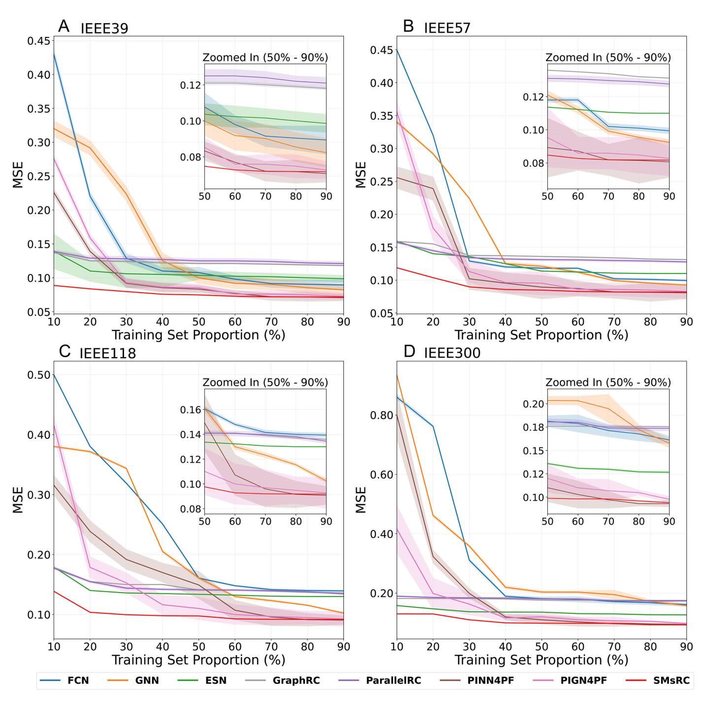
Figure 4. Comparison of MSE performance across four power grids. (A) IEEE39 bus system. (B) IEEE57 bus system. (C) IEEE118 bus system. (D) IEEE300 bus system. Shaded areas indicate the Standard Deviation (STD). Insets show magnified results for training set ratios of 50%–90% for clearer presentation.
Second, under data scarcity conditions, RC paradigm shows significant accuracy advantages over non-RC-based methods. This phenomenon can be explained from both architectural and theoretical perspectives. Architecturally, RC only trains the linear readout layer while keeping the reservoir weights fixed, which fundamentally reduces the number of learnable parameters and thus the sample complexity required for reliable generalization[52,53]. Theoretically, the reservoir serves as a high-dimensional nonlinear projection that maps input signals into a rich feature space where different system states become linearly separable[39,54]. This "separation property" enables the simple linear readout to distinguish complex patterns even with limited training samples. Furthermore, the fading memory property (echo state property) of the reservoir ensures that the network state is primarily determined by recent input history rather than requiring extensive data to learn temporal dependencies[37]. Recent studies have further demonstrated that RC can achieve effective predictions even from partial or incomplete observations[55], supporting its robustness in data-scarce scenarios. Consequently, while deep learning methods typically require large datasets for backpropagation-based gradient descent to converge reliably, RC circumvents this bottleneck through its fixed reservoir structure and linear training paradigm.
Third, for RC-based methods, when the amount of data is already sufficient, simply increasing the training samples does little to improve the performance of these models. However, the accuracy of GraphRC and ParallelRC is unsatisfactory, particularly when the training set ratio is higher. This can be attributed to their simple focus on individual nodes and their surroundings, while neglecting higher-order and system-wide information. Although this approach may be sufficient for local-related tasks, power flow calculations require a comprehensive understanding of interactions among bus nodes and the system′s overall physical characteristics. Additionally, their incorporation of physical mechanisms is relatively limited.
5.3. Parameter complexity and stable efficiency
First, as summarized in Table 2, this work analyzes the parameter complexity of each method under identical experimental settings, considering factors such as the number of neurons per layer or module and the number of grid buses. The table explicitly presents the parameter count expressions for each method, where
Comparison of parameter quantity for different methods. The last column represents the degree of improvement or decrease relative to the SMsRC
| Methods | Parameter count | Comparison |
| FCN | ||
| PINN4PF | ||
| GNN | ||
| PIGN4PF | ||
| ESN | ||
| GraphRC | ||
| ParallelRC | ||
| SMsRC |
Then, by fixing the training set ratio at 70%, the comparison of different methods in terms of efficiency with stability and precision is visually presented in Figure 5. It is clear that RC-based methods offer advantages in computational efficiency (i.e., lower running time) and stability (i.e., more consistent MSE values), while physics-informed methods excel in average prediction accuracy. The presented SMsRC framework effectively balances both, particularly standing out as the top performer in terms of both MSE and computational speed on the larger-scale IEEE300 system.
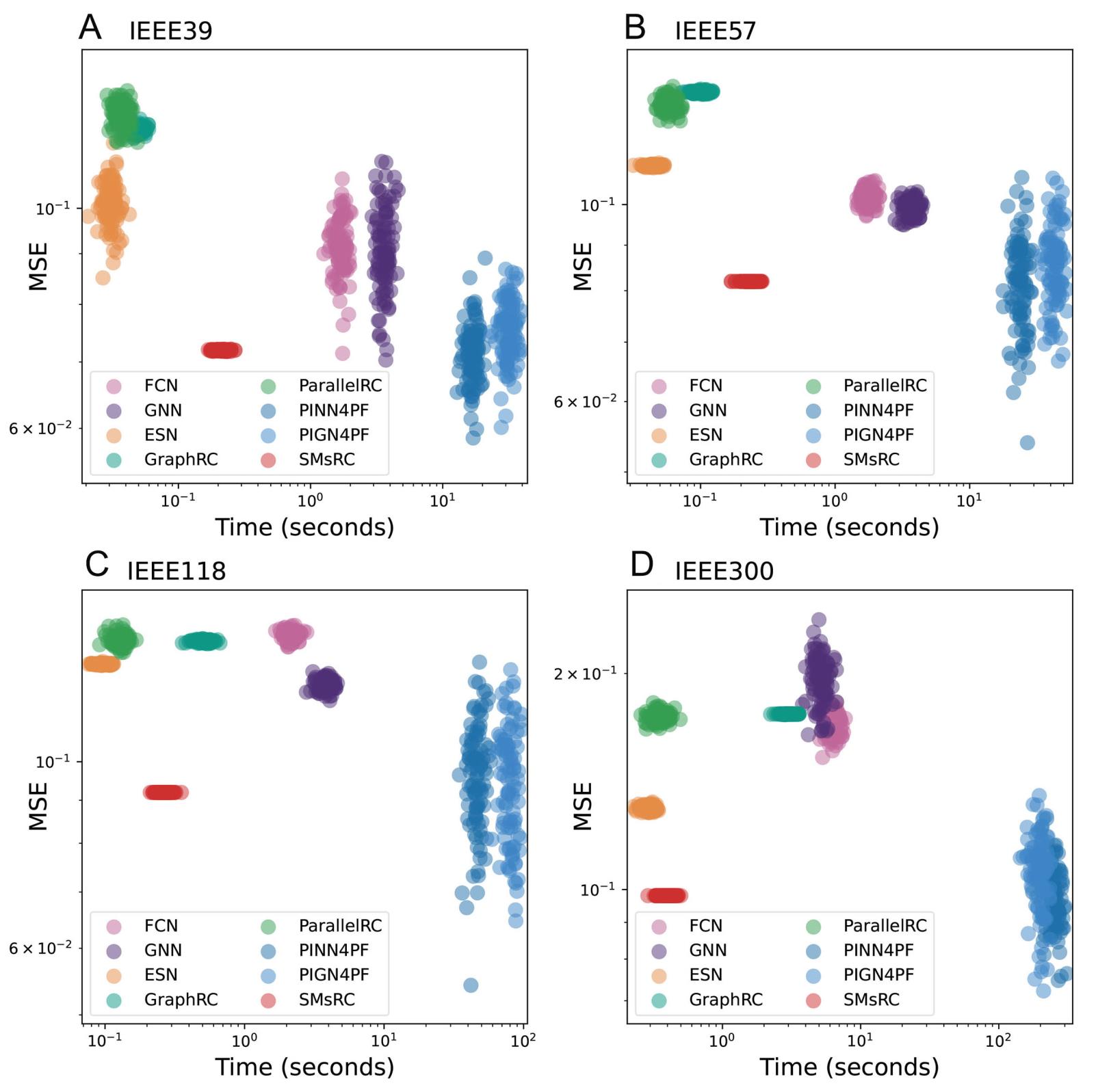
Figure 5. Comparison of efficiency, stability, and accuracy with a fixed training set ratio of 70%. (A) IEEE39 bus system. (B) IEEE57 bus system. (C) IEEE118 bus system. (D) IEEE300 bus system. Each cluster comprises 100 independent experiments, plotting running time (x-axis) against MSE (y-axis) to demonstrate computational speed and solution consistency.
5.4. Ablation experiments
The ablation experiments are conducted on the proposed SMsRC framework, as shown in Figure 6. In these experiments, "w/o FM" denotes the ablation of the functional matrix, meaning the random input matrix initialization method is retained. "w/o MS" represents the ablation of the spatial multi-scale component, which effectively reduces the three reservoirs in Figure 1(e) to a single reservoir while maintaining the same total number of reservoir nodes, and it includes "w/o PI" and "w/o HB". "w/o PI" indicates that the framework does not incorporate physical information and relies solely on sample data, with spatial multi-scale information aggregation limited to a simple summation of neighboring attributes. Last, "w/o HB" signifies that the framework no longer uses higher-order neighbor information of buses, considering only topologically first-order neighbors.
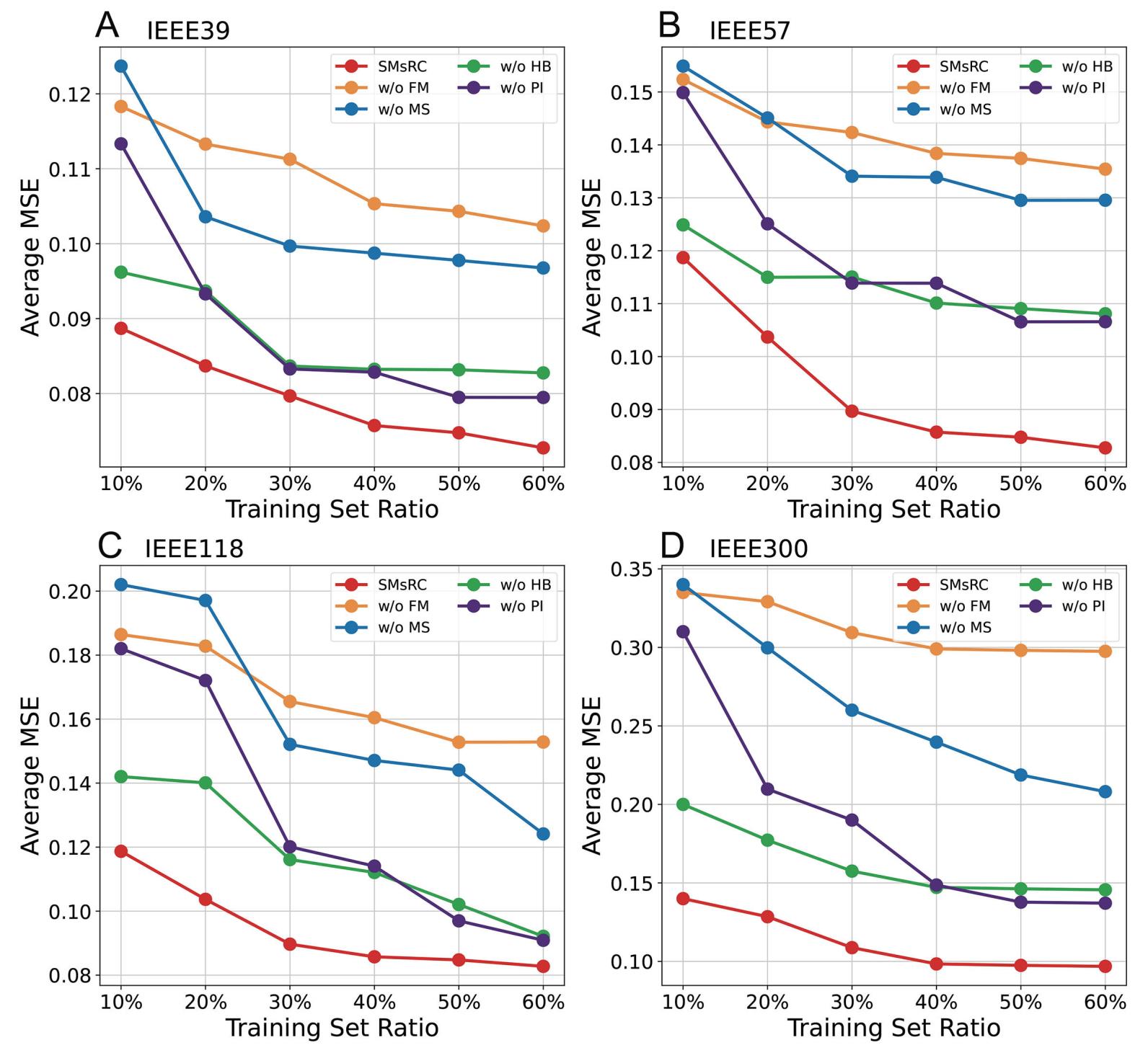
Figure 6. Average MSE of various ablation methods across different datasets. (A) IEEE39 bus system. (B) IEEE57 bus system. (C) IEEE118 bus system. (D) IEEE300 bus system. The ablation settings are defined as: "w/o FM" (without functional matrix), "w/o MS" (without spatial multi-scale mechanism), "w/o PI" (without physical information integration), and "w/o HB" (without higher-order neighbor mining).
In terms of prediction accuracy, the functional matrix and spatial multi-scale are the most critical contributors to the framework, followed by higher-order neighbors and physical information. Additionally, spatial multi-scale and physical information can further enhance stability in data-scarce scenarios. This is evidenced by the steeper curves for the "w/o PI" and "w/o MS" ablation studies, signifying a less stable model transition from data scarcity to normal conditions, and the "w/o MS" setup typically performs worst when the amount of data is minimal.
From a theoretical standpoint, the ablation results validate that each proposed component contributes to enhanced data efficiency in distinct ways. The functional matrix, by encoding deterministic bus-specific roles rather than random weights, provides structured inductive biases that reduce the hypothesis space the model must explore, thereby requiring fewer samples to identify correct mappings[38]. The spatial multi-scale mechanism aggregates information from higher-order neighbors, effectively increasing the information content available per sample by exploiting the inherent correlations in the power grid topology[55]. Finally, the integration of physical information acts as domain-specific regularization, constraining the solution space to physically plausible outputs and preventing overfitting in low-data regimes[56]. These three mechanisms synergistically enhance the framework′s sample efficiency, enabling robust performance even when only limited operational data is available.
5.5. Case analysis
Finally, a case study conducted on the 39-bus system in New England is presented in Figure 7. Specifically, Figure 7B-D shows the absolute errors between the model outputs and the true system values: (b)
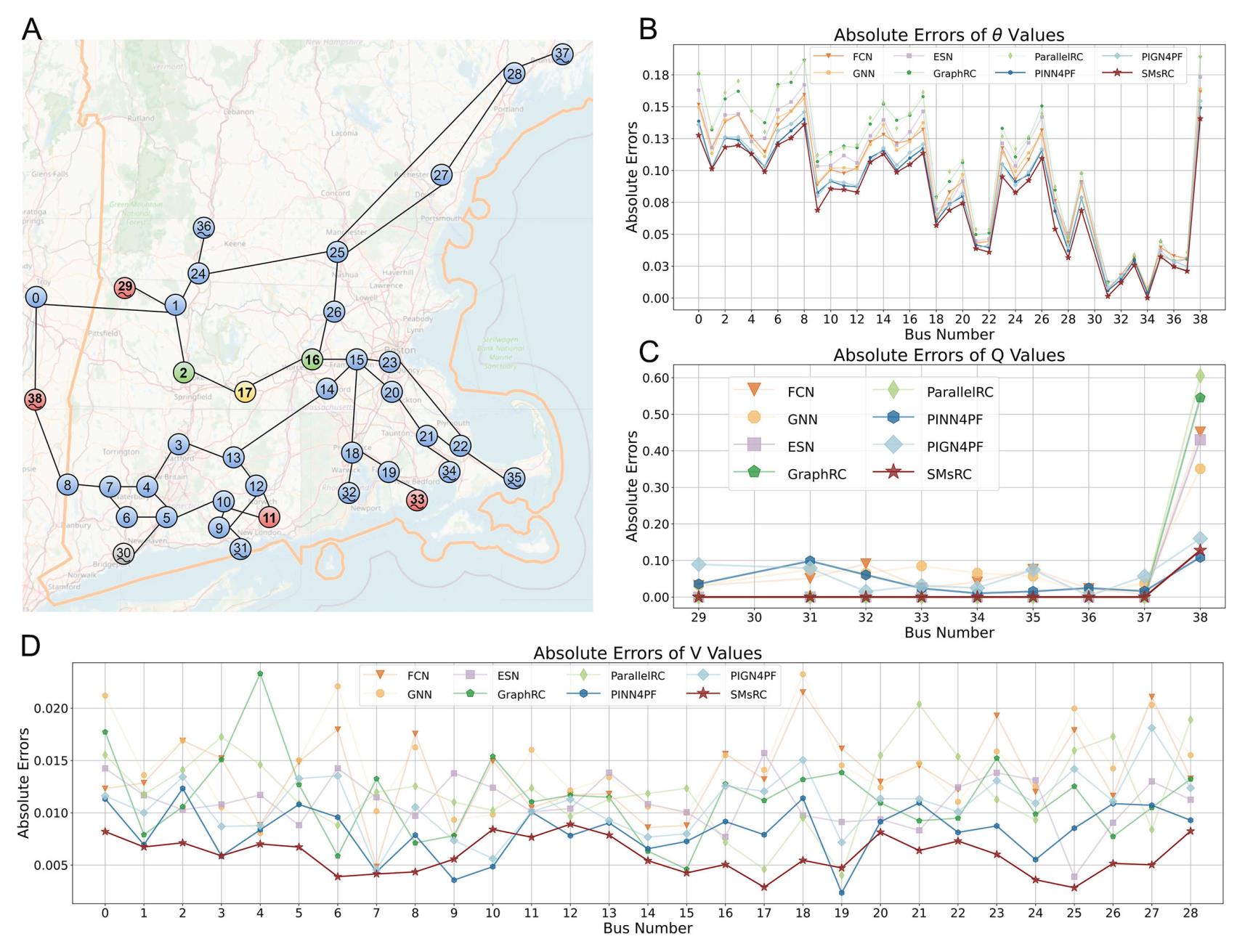
Figure 7. Case analysis of IEEE39 system located in New England. (A) The geographical distribution and connection relationships of 39 buses (Map data ©OpenStreetMap contributors). Green nodes are the direct neighbors of bus 17, and red nodes are the higher-order neighbors of bus 17 identified by SMsRC. (B-D) denote the absolute errors between the model outputs and the true system values for
6. CONCLUSIONS
In this work, we leverage the RC paradigm, proposing a SMsRC framework that integrates a functional matrix and physical information. The framework is structured into three main computational stages: parallel learning of auxiliary information, reconstructing the input matrix and input information, and a spatial multi-scale reservoir with a physically constrained readout layer. Together, these stages form a complete and robust power flow solution approach. The main experiments conducted on four standard IEEE bus systems comprehensively validate the effectiveness and advantages of the SMsRC as a power flow solver in terms of computational efficiency, accuracy, generalizability, and robustness. Ablation experiments also validate the critical role of each component.
In future work, we aim to further enhance the presented framework from other perspectives. However, there are still some limitations in this work that merit further investigation. First, regarding the mining of higher-order relationships, the current framework relies on the BPLoss metric. While effective, this metric infers dependencies indirectly based on pairwise prediction errors, and may not fully capture the complex, multi-way interactions inherent in power grid topologies as explicitly as advanced graph-theoretic tools such as hypergraphs or motifs. Second, although the framework demonstrates robustness in data-scarce scenarios, the current study primarily focuses on power flow calculations under steady-state conditions. It has not yet addressed the power flow solvability under scenarios involving dynamic or uncertain factors, such as time-varying load fluctuations, renewable energy intermittency, or extreme events including complex perturbations and cascading failures. Incorporating such factors into the physical constraints would require extending the current static constraint formulation to probabilistic or time-dependent forms, for example, by introducing stochastic programming or robust optimization techniques within the readout layer. Addressing these limitations by integrating hypergraph theory, developing uncertainty-aware physical constraints, and extending the framework to dynamic resilience analysis will be the focus of our future research.
DECLARATIONS
Authors′ contributions
Methodology, visualization, and writing-original draft: Zhang, H. F.; Zhang, Y. M.; Ding, X.; Ma, C.
Conceptualization, validation, writing-reviewing, and supervision: Xia, Y.; Tse, C. K.
Availability of data and materials
The raw data supporting the conclusions of this article will be made available by the authors upon request.
Financial support and sponsorship
This work is supported by the National Natural Science Foundation of China (62473001, 62476002), the Hong Kong Research Grants Council under GRF 112015/24, and the City University of Hong Kong (Grant No. 9229105).
Conflicts of interest
All authors declared that there are no conflicts of interest.
Ethical approval and consent to participate
Not applicable.
Consent for publication
Not applicable.
Copyright
© The Author(s) 2026.
REFERENCES
1. Rahman, M.; Islam, M. R.; Hossain, M. A.; Rana, M.; Hossain, M.; Gray, E. M. Resiliency of forecasting methods in different application areas of smart grids: a review and future prospects. Eng. Appl. Artif. Intell. 2024, 135, 108785.
2. Judge, M. A.; Khan, A.; Manzoor, A.; Khattak, H. A. Overview of smart grid implementation: frameworks, impact, performance and challenges. J. Energy. Storage. 2022, 49, 104056.
3. Lopez-Garcia, T. B.; Dominguez-Navarro, J. A. Power flow analysis via typed graph neural networks. Eng. Appl. Artif. Intell. 2023, 117, 105567.
4. Glover, J. D.; Sarma, M. S.; Overbye, T. Power system analysis and design, 6th ed. Stamford, CT: CengageLearning; 2017.
5. Milano, F. Continuous newton′s method for power flow analysis. IEEE. Trans. Power. Syst. 2009, 24, 50-7.
6. Huang, S.; Wang, L.; Xiong, L.; et al. Hierarchical robustness strategy combining model-free prediction and fixed-time control for islanded AC microgrids. IEEE. Trans. Smart. Grid. 2025, 16, 4380-94.
7. Ding, X.; Wang, H.; Zhang, X.; Ma, C.; Zhang, H. Dual nature of cyber–physical power systems and the mitigation strategies. Reliab. Eng. Syst. Saf. 2024, 244, 109958.
8. Khaloie, H.; Dolányi, M.; Toubeau, J.; Vallee, F. Review of machine learning techniques for optimal power flow. Appl. Energy. 2025, 388, 125637.
9. Pineda, S.; Perez-ruiz, J.; Morales, J. M. Beyond the neural fog: interpretable learning for AC optimal power flow. IEEE. Trans. Power. Syst. 2025, 40, 4912-21.
10. Canyasse, R.; Dalal, G.; Mannor, S. Supervised learning for optimal power flow as a real-time proxy. In 2017 IEEE Power & Energy Society Innovative Smart Grid Technologies Conference (ISGT), Washington, DC, USA, April 23-26, 2017; pp 1-5.
11. Ng, Y.; Misra, S.; Roald, L. A.; Backhaus, S. Statistical learning for DC optimal power flow. In 2018 Power Systems Computation Conference (PSCC), Dublin, Ireland, June 11-15, 2018; pp 1-7.
12. Liu, C.; Li, Y.; Xu, T. A neural network approach to physical information embedding for optimal power flow. Sustainability 2024, 16, 7498.
13. Grigoras, G.; Cartina, G.; Bobric, E.; Barbulescu, C. Missing data treatment of the load profiles in distribution networks. In 2009 IEEE Bucharest PowerTech (POWERTECH), Bucharest, Romania, June 28-July 2, 2009; pp 1-5.
14. Wringe, C.; Trefzer, M.; Stepney, S. Reservoir computing benchmarks: a tutorial review and critique. Int. J. Parallel. Emergent. Distrib. Syst. 2025, 40, 313-51.
15. Li, X.; Zhu, Q.; Zhao, C.; et al. Tipping point detection using reservoir computing. Research 2023, 6, 0174.
16. Sakemi, Y.; Morino, K.; Leleu, T.; Aihara, K. Model-size reduction for reservoir computing by concatenating internal states through time. Sci. Rep. 2020, 10, 21794.
17. Gao, L.; Deng, X.; Yang, W. Smart city infrastructure protection: real-time threat detection employing online reservoir computing architecture. Neural. Comput. Applic. 2021, 34, 833-42.
18. Yang, C.; Sun, Y.; Zou, Y.; et al. Optimal power flow in distribution network: a review on problem formulation and optimization methods. Energies 2023, 16, 5974.
19. Grisales-Norena, L. F.; Montoya, O. D.; Gil-Gonzalez, W. J.; Perea-Moreno, A.; Perea-Moreno, M. A comparative study on power flow methods for direct-current networks considering processing time and numerical convergence errors. Electronics 2020, 9, 2062.
20. Niu, Z.; Zhang, C.; Li, Q.; Liu, X. Power flow calculation of small impedance branches system based on improved rectangular coordinate newton method. In 2022 5th International Conference on Electronics and Electrical Engineering Technology (EEET), Beijing, China, December 2-4, 2022; pp 110-9.
21. Montoya, O. D. On the existence of the power flow solution in DC grids with CPLs through a graph-based method. IEEE. Trans. Circuits. Syst. II. 2020, 67, 1434-8.
22. Tang, Y.; Dvijotham, K.; Low, S. Real-time optimal power flow. IEEE. Trans. Smart. Grid. 2017, 8, 2963-73.
23. Niu, M.; Wan, C.; Xu, Z. A review on applications of heuristic optimization algorithms for optimal power flow in modern power systems. J. Mod. Power. Syst. Clean. Energy. 2014, 2, 289-97.
24. Cui, T.; Wang, S.; Qu, Y.; Chen, X. Parameters optimization of electro-hydraulic power steering system based on multi-objective collaborative method. Complex. Eng. Syst. 2023, 3, 2.
25. Bakirtzis, A.; Biskas, P.; Zoumas, C.; Petridis, V. Optimal power flow by enhanced genetic algorithm. IEEE. Trans. Power. Syst. 2002, 17, 229-36.
26. Ghasemi, M.; Taghizadeh, M.; Ghavidel, S.; Aghaei, J.; Abbasian, A. Solving optimal reactive power dispatch problem using a novel teaching–learning-based optimization algorithm. Engineering. Applications. of. Artificial. Intelligence. 2015, 39, 100-8.
27. Papadimitrakis, M.; Giamarelos, N.; Stogiannos, M.; Zois, E.; Livanos, N.; Alexandridis, A. Metaheuristic search in smart grid: a review with emphasis on planning, scheduling and power flow optimization applications. Renew. Sustain. Energy. Rev. 2021, 145, 11072.
28. Stankovic, S.; Söder, L. Optimal power flow based on genetic algorithms and clustering techniques. In 2018 Power Systems Computation Conference (PSCC), Dublin, Ireland, June 11-15, 2018; pp 1-7.
29. Huang, W.; Pan, X.; Chen, M.; Low, S. H. DeepOPF-Ⅴ: solving AC-OPF problems efficiently. IEEE. Trans. Power. Syst. 2022, 37, 800-3.
30. Bottcher, L.; Wolf, H.; Jung, B.; et al. Solving AC power flow with graph neural networks under realistic constraints. In 2023 IEEE Belgrade PowerTech, Belgrade, Serbia, June 25-29, 2023; pp 1-7.
31. Zhang, H. F.; Lu, X. L.; Ding, X.; Zhang, X. M. Physics-informed line graph neural network for power flow calculation. Chaos 2024, 34, 113123.
32. Hansen, J. B.; Anfinsen, S. N.; Bianchi, F. M. Power flow balancing with decentralized graph neural networks. IEEE. Trans. Power. Syst. 2023, 38, 2423-33.
33. Zhou, Y.; Lee, W.; Diao, R.; Shi, D. Deep reinforcement learning based real-time AC optimal power flow considering uncertainties. J. Mod. Power. Syst. Clean. Energy. 2022, 10, 1098-109.
34. Nellikkath, R.; Chatzivasileiadis, S. Physics-informed neural networks for AC optimal power flow. Elect. Power. Syst. Res. 2022, 212, 108412.
35. Singh, M. K.; Kekatos, V.; Giannakis, G. B. Learning to solve the AC-OPF using sensitivity-informed deep neural networks. IEEE. Trans. Power. Syst. 2022, 37, 2833-46.
36. Yan, M.; Huang, C.; Bienstman, P.; Tino, P.; Lin, W.; Sun, J. Emerging opportunities and challenges for the future of reservoir computing. Nat. Commun. 2024, 15, 2056.
37. Yildiz, I. B.; Jaeger, H.; Kiebel, S. J. Re-visiting the echo state property. Neural. Netw. 2012, 35, 1-9.
38. Lukoševičius, M. A practical guide to applying echo state networks. Berlin Heidelberg: Springer; 2012; pp 659-86.
39. Jaeger, H. The "echo state" approach to analysing and training recurrent neural networks – with an Erratum note. 2001.
40. Wood, A. J.; Wollenberg, B. F.; Sheblé, G. B. Power generation, operation, and control, 3rd ed. Hoboken, NJ: John Wiley & Sons; 2013.
41. Watts, D. J.; Strogatz, S. H. Collective dynamics of ′small-world′ networks. Nature 1998, 393, 440-2.
42. Emelianova, A. A.; Maslennikov, O. V.; Nekorkin, V. I. Higher-order interactions, adaptivity, and phase transitions in a novel reservoir computing model. Chaos 2025, 35, 103110.
43. Keriven, N. Not too little, not too much: a theoretical analysis of graph (over) smoothing. Adv. Neural. Inf. Process. Syst. 2022, 35, 2268-81.
44. Birchfield, A. B.; Xu, T.; Gegner, K. M.; Shetye, K. S.; Overbye, T. J. Grid structural characteristics as validation criteria for synthetic networks. IEEE. Trans. Power. Syst. 2017, 32, 3258-65.
45. Thurner, L.; Scheidler, A.; Schafer, F.; et al. Pandapower - an open-source python tool for convenient modeling, analysis, and optimization of electric power systems. IEEE. Trans. Power. Syst. 2018, 33, 6510-21.
46. Yang, Y.; Yang, Z.; Yu, J.; Zhang, B.; Zhang, Y.; Yu, H. Fast calculation of probabilistic power flow: a model-based deep learning approach. IEEE. Trans. Smart. Grid. 2020, 11, 2235-44.
47. Owerko, D.; Gama, F.; Ribeiro, A. Optimal power flow using graph neural networks. In ICASSP 2020 - 2020 IEEE International Conference on Acoustics, Speech and Signal Processing (ICASSP), Barcelona, Spain, May 4-8, 2020; pp 5930-4.
48. Gallicchio, C.; Micheli, A. Graph echo state networks. In 2010 International Joint Conference on Neural Networks (IJCNN), Barcelona, Spain, July 18-23, 2010; pp 1-8.
49. Srinivasan, K.; Coble, N.; Hamlin, J.; Antonsen, T.; Ott, E.; Girvan, M. Parallel machine learning for forecasting the dynamics of complex networks. Phys. Rev. Lett. 2022, 128, 164101.
50. Gao, M.; Yu, J.; Yang, Z.; Zhao, J. Physics embedded graph convolution neural network for power flow calculation considering uncertain injections and topology. IEEE. Trans. Neural. Netw. Learn. Syst. 2024, 35, 15467-78.
51. Wang, J.; Srikantha, P. Data-driven AC optimal power flow with physics-informed learning and calibrations. In 2024 IEEE International Conference on Communications, Control, and Computing Technologies for Smart Grids (SmartGridComm), Oslo, Norway, September 17-20, 2024; pp 289-94.
52. Lukoševičius, M.; Jaeger, H. Lukoševičius reservoir computing approaches to recurrent neural network training. Comput. Sci. Rev. 2009, 3, 127-49.
53. Gauthier, D. J.; Bollt, E.; Griffith, A.; Barbosa, W. A. S. Next generation reservoir computing. Nat. Commun. 2021, 12, 5564.
54. Dambre, J.; Verstraeten, D.; Schrauwen, B.; Massar, S. Information processing capacity of dynamical systems. Sci. Rep. 2012, 2, 514.
55. Ratas, I.; Pyragas, K. Application of next-generation reservoir computing for predicting chaotic systems from partial observations. Phys. Rev. E. 2024, 109, 064215.
Cite This Article
How to Cite
Download Citation
Export Citation File:
Type of Import
Tips on Downloading Citation
Citation Manager File Format
Type of Import
Direct Import: When the Direct Import option is selected (the default state), a dialogue box will give you the option to Save or Open the downloaded citation data. Choosing Open will either launch your citation manager or give you a choice of applications with which to use the metadata. The Save option saves the file locally for later use.
Indirect Import: When the Indirect Import option is selected, the metadata is displayed and may be copied and pasted as needed.
About This Article
Special Topic
Copyright

Data & Comments
Data
0


Comments
Comments must be written in English. Spam, offensive content, impersonation, and private information will not be permitted. If any comment is reported and identified as inappropriate content by OAE staff, the comment will be removed without notice. If you have any queries or need any help, please contact us at [email protected].