

Configuration selection and matrix-aware optimization for data-efficient atomistic foundation models
 0

Graphical Abstract
Abstract
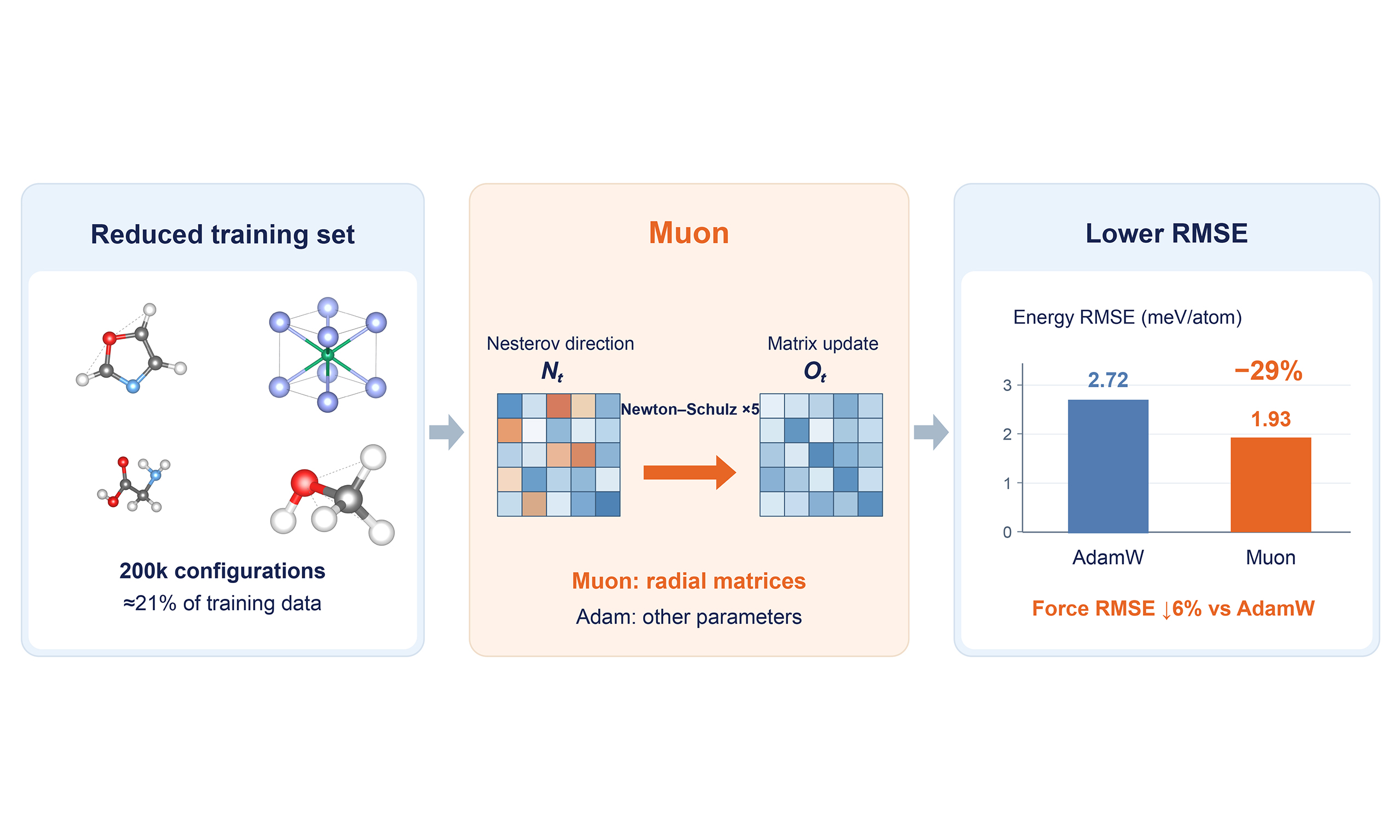
Atomistic foundation models achieve high accuracy by training on very large labeled datasets. However, it remains unclear how much of this data is actually needed. Data-efficient training requires a better understanding of the roles of both data selection and model optimization. Here, we study these two factors separately using MACE-OFF24 as a baseline. We build smaller training sets by selecting configurations to cover diverse local atomic environments and include cases with large teacher-model errors. We then compare AdamW with the matrix-aware Muon optimizer using the same training data. We selected approximately 21% of the available configurations (190,000 for training and 10,000 for validation). Training from scratch produced energy and force root-mean-square errors within 8.1% and 6% of those obtained with the published checkpoint. On the fixed 200k subset, Muon reduced mean energy and force errors by 29% and 6% relative to AdamW. In a single-run comparison of selection rules within a fixed candidate pool at 49k, the 80:20 representative/residual allocation gave the lowest observed energy and force errors. On a separate small test set of approximately 7,000 3BPA conformers, AdamW instead gave the lowest mean relative-energy and energy-span errors. Our results show that data-efficient training of atomistic foundation models is jointly controlled by configuration coverage, optimizer geometry, chemical regime, and target observable. Especially, for training on big datasets, matrix-aware updates can improve broad from-scratch energy-force training.
Keywords


 Download PDF
INTRODUCTION
Machine-learning interatomic potentials (MLIPs) replace repeated electronic-structure calculations with learned energy and force models, extending molecular and materials simulation to larger systems and longer time scales[1-10]. Equivariant representations have improved data efficiency and enabled scalable atomistic simulation[11,12]. Equivariant graph neural networks have extended this approach to universal or foundation MLIPs (U-MLIPs) trained across broad chemical spaces[13-18]. These models can serve as reusable components of high-throughput computational chemistry and materials modeling, but their chemical breadth relies on large, heterogeneous training collections. Efficiently reusing these labeled collections in smaller subsets is therefore important for making foundation-model training and adaptation more economical while preserving the chemical coverage required for downstream simulation[19]. Against this background, the problem considered here is the retrospective reduction of an existing, fully labeled atomistic dataset. Every retained configuration keeps its energy and complete force array, so removing a record removes both its supervision and the chemical environment it represents. For a fixed model architecture, the error obtained from such a reduced training set depends jointly on which configurations are retained and how the model is optimized. A learning curve that varies only the number of configurations leaves these effects confounded: the same subset can yield different errors under different optimizer configurations, while equal-size subsets can yield different errors under the same optimizer. The central problem is therefore not simply to find the smallest subset that reaches an aggregate error threshold, but to separate configuration coverage from optimization and determine the chemical regimes and observables for which accuracy is retained.
Relevant work falls into two broad strands. The first studies which data or labels should be retained. Sparse-label studies keep configurations but remove selected targets such as forces, whereas active-learning methods select configurations for new reference calculations by combining uncertainty, diversity, and iterative exploration[20-27]. Data-curation methods can instead construct compact training sets from existing labeled collections or identify diverse and discrepancy-aware subsets before new calculations[28-30], while application-specific studies may jointly vary label fidelity, model expressivity, and training-set size[31]. The second strand studies how optimization affects atomistic and geometric networks. We benchmarked first-order optimizers and a limited-memory Broyden–Fletcher–Goldfarb–Shanno (L-BFGS) refinement stage for fine-tuning pretrained atomistic foundation models[32]. Harari et al. compared the Muon, SOAP, and SOAP–Muon optimizers with AdamW under partial force supervision[33], while other studies have examined optimizer-dependent accuracy, loss geometry, spectral rank, and the basis covariance of polar updates[34,35].
However, these two strands remain largely separate. Offline curation studies do not establish how optimization affects models trained after complete configurations have been removed, while existing optimizer studies focus on fine-tuning, partial force supervision, or optimizer-dependent geometry without controlling configuration selection. They therefore do not show whether reduced-data accuracy comes from the selected configurations, the optimization protocol, or an interaction between the two. Nor do they connect matrix-aware updates to the energy and force outputs of the specific architecture being trained. The interaction between complete-configuration selection, optimization, and chemically resolved accuracy consequently remains unresolved.
In this work, we address this gap using MACE-OFF24 as a large-scale benchmark[36]. We construct reduced, fully labeled training sets by combining local-environment coverage within configuration families with teacher-residual enrichment. We then separate the two factors through complementary comparisons. One holds the selected configurations fixed while varying the complete optimizer configuration. The other fixes the optimization protocol, data count, and label-aware candidate pool while varying within-cluster selection. Aggregate and chemical-split errors assess where accuracy is retained, while a 3BPA conformational-energy test probes transfer to a chemically interpretable observable. This study demonstrates that multi-atomic cluster expansion (MACE) trained from scratch on the training partition of the selected 21% subset approaches the reference accuracy of MACE-OFF24 with full labels, while disentangling the respective effects of optimizer configurations and data selection rules, and mechanistically linking Muon-updated radial matrices to energy and force outputs via operator analysis. Together, this design treats efficient reuse of atomistic data as a joint question of configuration coverage, optimization, and the target chemical regime and observable.
MATERIALS AND METHODS
Model architecture and training objective
We use MACE as the equivariant MLIP architecture for the controlled study[37]. MACE encodes atomic neighborhoods through a body-ordered atomic-cluster expansion and propagates information with tensor products between learned radial features and equivariant spherical-harmonic basis functions, followed by symmetrized contractions over angular channels up to maximum angular degree ℓmax. The resulting node features pass through a learnable readout that produces per-atom energies; atomic forces follow by analytic differentiation of the predicted potential energy with respect to atomic positions.
The controlled benchmark runs used a two-block MACE configuration with 128 channels, ℓmax = 1, correlation order three, and maximum neighbor distance rmax = 6.0 Å. This architecture matches the published full-data reference, whose checkpoint is evaluated on the same official test splits and used as the accuracy target in the size-scaling benchmark. Training used double precision. Each selected OFF24 subset used a 95:5 training/validation split; the 200k subset therefore corresponds to 190,000 training and 10,000 validation configurations. Atomic-energy offsets, normalization, and neighbor statistics were fitted only on its training partition. The fixed-200k comparison reused one prepared split and its statistics across optimizers and training runs; the five 49k subsets shared the splitting rule, with statistics fitted separately for each subset.
Training objective and schedule. The scalar training loss
The force threshold depends on the magnitude of the reference force vector, while the two-stage schedule shifts weight from forces toward energies late in training. The OFF24 comparisons used this objective and schedule with validation-based checkpoint selection; the separate 3BPA transfer protocol is described in Section “Transfer Evaluation”.
Structured subset construction
Let the labeled training set contain N configurations and be written as
where i ∈ {1, …, N} indexes a configuration, xi contains its atomic species and coordinates, Ei is its scalar reference energy, and Fi is its full array of Cartesian force components. We choose an index set S
No target is masked within a selected tuple. The retained fraction is m/N, and the ratio of the original to retained set sizes is N/m. This differs from force-label sparsification, which retains all configurations but introduces a force mask in the loss for some of them.
Let
The minimization considers all index sets S of size m to identify the subset with the lowest target risk after training. In the experiments, energy and force root mean square error (RMSE) are evaluated separately on the untouched official test set
To make the dependence on training explicit, we denote the comparison risk for subset S and protocol
At fixed S, two protocols
The public benchmark corpus contains 951,005 configurations across seven chemical families and defines the denominator for all retained-data fractions[36]. We form a label-aware candidate pool containing approximately 31.5% of the benchmark corpus by stratifying over configuration family and size, preserving elemental coverage, and enriching configurations with large teacher residuals. This stage reduces the cost of descriptor construction, principal component analysis (PCA), clustering, and quota assignment; the same selector can instead act on the full collection by setting
Local-environment representation. Each configuration is represented by aggregated local descriptors that encode the central element, radial-shell neighbor composition and coordination, neighbor-distance statistics, and configuration size.
Representative and residual selection. Standardized descriptors are projected using PCA and clustered within configuration families. Representative ranks favor configurations spread across each cluster; residual ranks favor large teacher energy and force errors. The residual score for configuration c is
where
Muon optimization and matrix-update analysis
For Wt-1 ∈
Here, Mt is the momentum matrix at iteration t, formed as an exponential moving average of the gradients. The coefficients (a, b, c) = (3.4445, -4.7750, 2.0315) are adopted from Muon, where they were numerically selected to increase the polynomial’s slope near zero and accelerate approximate orthogonalization[38].
Matrix scope in MACE. Muon updates eight matrices that generate radial coefficients for tensor-product messages. We compare it with AdamW[39] and ScheduleFree[40].
Optimizer settings. The optimizer settings were fixed without a matched tuning search at 200k. Before stage two, Muon and AdamW used plateau-based learning-rate reduction; ScheduleFree did not. All three used the same stage-two learning-rate schedule.
Controlled benchmark runs. The 200k comparison used three paired training runs and the common training protocol in Section “Model architecture and training objective”. The 49k arms shared initialization and data-ordering settings, the label-aware pool, anchors, PCA representation, clusters, family and cluster quotas, Muon protocol, 200 epochs, and test set. Only within-cluster selection varied: matched random, representative-only, residual-only, and 80:20 or 50:50 representative/residual mixtures. To relate radial-matrix updates to MACE outputs, we bound perturbations in radial coefficients, tensor-product messages, energies, and forces. For radial layer l, Wl is the coefficient matrix, al(r) its input activation, and
Here, Δcl(r) denotes the change in radial coefficients at distance r induced by the matrix perturbation ΔWl, with al(r) held fixed. For matrices, ||·||2 is the operator norm: the largest singular value or maximum amplification. Tensor-product messages depend linearly on radial coefficients, so their perturbations are controlled by the same matrix norm. For a fixed configuration and sufficiently small ΔWl,
where Fα = -∂E/∂Rα and ||·||* is the nuclear norm, the sum of the singular values. For a nonzero matrix direction G =
The polar direction maximizes alignment within an operator-norm bound; Muon approximates it using the five-step polynomial in Equation (7).
Transfer evaluation
For 3BPA[42], AdamW, ScheduleFree, and Muon were compared over three paired training runs starting from the published MACE-OFF24 medium checkpoint[36], without stochastic weight averaging. All 7,047 dihedral conformers were evaluated using the same protocol. Relative energies (kcal/mol) were obtained by subtracting each model’s prediction for the density functional theory (DFT) minimum-energy conformer. For each run, we computed predicted-minus-DFT relative-energy residuals and their mean, and recorded the energies and conformer identities of the predicted extrema. Mean absolute error (MAE) differences were decomposed over DFT-energy intervals [0, 2), [2, 5), [5, 10), [10, 15), and [15, ∞) kcal/mol. Each interval contributes its population fraction times the within-interval MAE difference. Median-centering subtracts each run’s median residual before recomputing MAE.
RESULTS AND DISCUSSION
Effect of selected-subset size on MACE-OFF24
We first measure the accuracy of the combined selection and training procedure as the number of selected configurations increases. We then hold either the training set or the optimization protocol fixed to separate their effects. Finally, split-wise and conformational evaluations show where the aggregate trends hold and where the optimizer ranking changes. In the first experiment, the Muon optimization protocol is fixed, the target selected-subset size varies from 25k to 200k configurations, and MACE is trained from scratch at each size. The 25k, 100k, 150k, and 200k subsets use the PCA selector, whereas the 49k point is the historical pre-PCA 70:30 realization. Mean energy and force RMSE decrease monotonically across the five target sizes [Figure 1 and Table 1]. At 200k configurations, or 21% of the available benchmark corpus, energy and force RMSE are within 8.1% and 6%, respectively, of those obtained with the published full-data checkpoint. The 25k and historical 49k models remain well above the published reference, the 100k model is intermediate, and the 150k and 200k models approach it. Across these target sizes, the energy gap closes more rapidly than the force gap. This curve describes the combined effect of data count and subset realization.
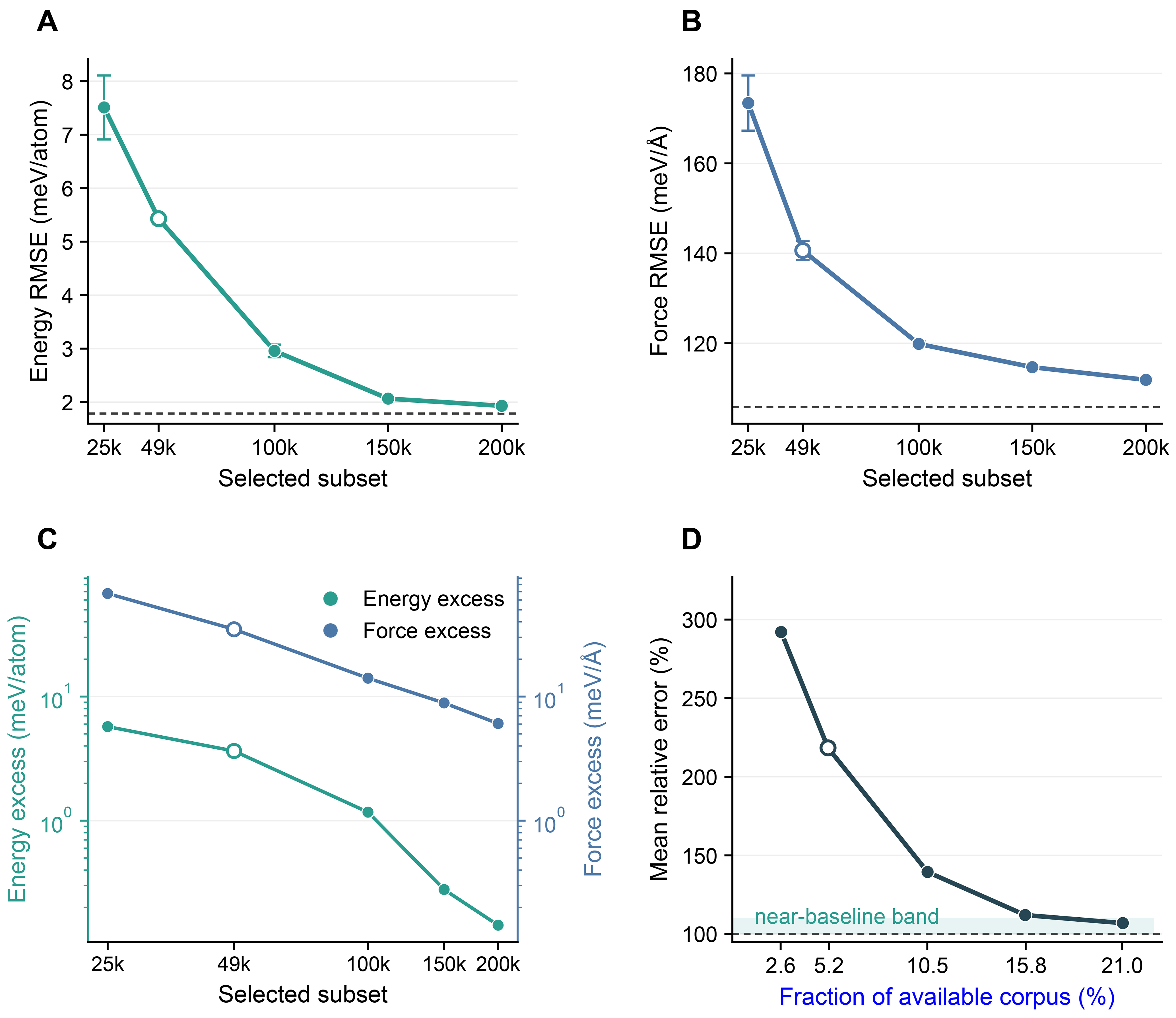
Figure 1. MACE-OFF24 target-size benchmark with the Muon optimization protocol held fixed. (A and B) show overall energy and force RMSE as the fully labeled selected subset increases from 25k to 200k configurations, with error bars denoting sample standard deviations over three training runs. Dashed horizontal lines in (A) and (B) mark the published full-data references; (C) shows energy excess on the left axis (meV/atom) and force excess on the right axis (meV/Å), both on logarithmic scales; connecting lines are visual guides; (D) shows the mean of the energy and force RMSE ratios relative to the references, with a dashed horizontal line at 100% and a shaded band from 100% to 110%. The open 49k marker identifies the historical pre-PCA 70:30 realization; the other reduced-data points use the PCA selector. MACE: Multi-atomic cluster expansion; RMSE: root mean square error; PCA: principal component analysis.
Overall MACE-OFF24 test performance with the Muon optimization protocol
| Model (selected-subset size; corpus fraction) | Energy RMSE (meV/atom) | Force RMSE (meV/Å) |
| Published MACE-OFF24 reference | 1.79 | 105.79 |
| 25k structured (25,000; 2.6%) | 7.51 ± 0.60 (+320%) | 173.41 ± 6.14 (+64%) |
| 49k historical pre-PCA (49,000; 5.2%) | 5.43 ± 0.04 (+204%) | 140.63 ± 2.14 (+33%) |
| 100k structured (100,000; 10.5%) | 2.96 ± 0.12 (+66%) | 119.85 ± 0.56 (+13%) |
| 150k structured (150,000; 15.8%) | 2.07 ± 0.02 (+16%) | 114.68 ± 0.28 (+8%) |
| 200k structured (200,000; 21.0%) | 1.93 ± 0.02 (+8%) | 111.86 ± 0.30 (+6%) |
Separating optimization and configuration-selection effects
Muon, AdamW, and ScheduleFree each use the same 200k structured subset, architecture, loss function, 200-epoch budget, and evaluation set and are each evaluated in three replicate runs [Figure 2 and Table 2].
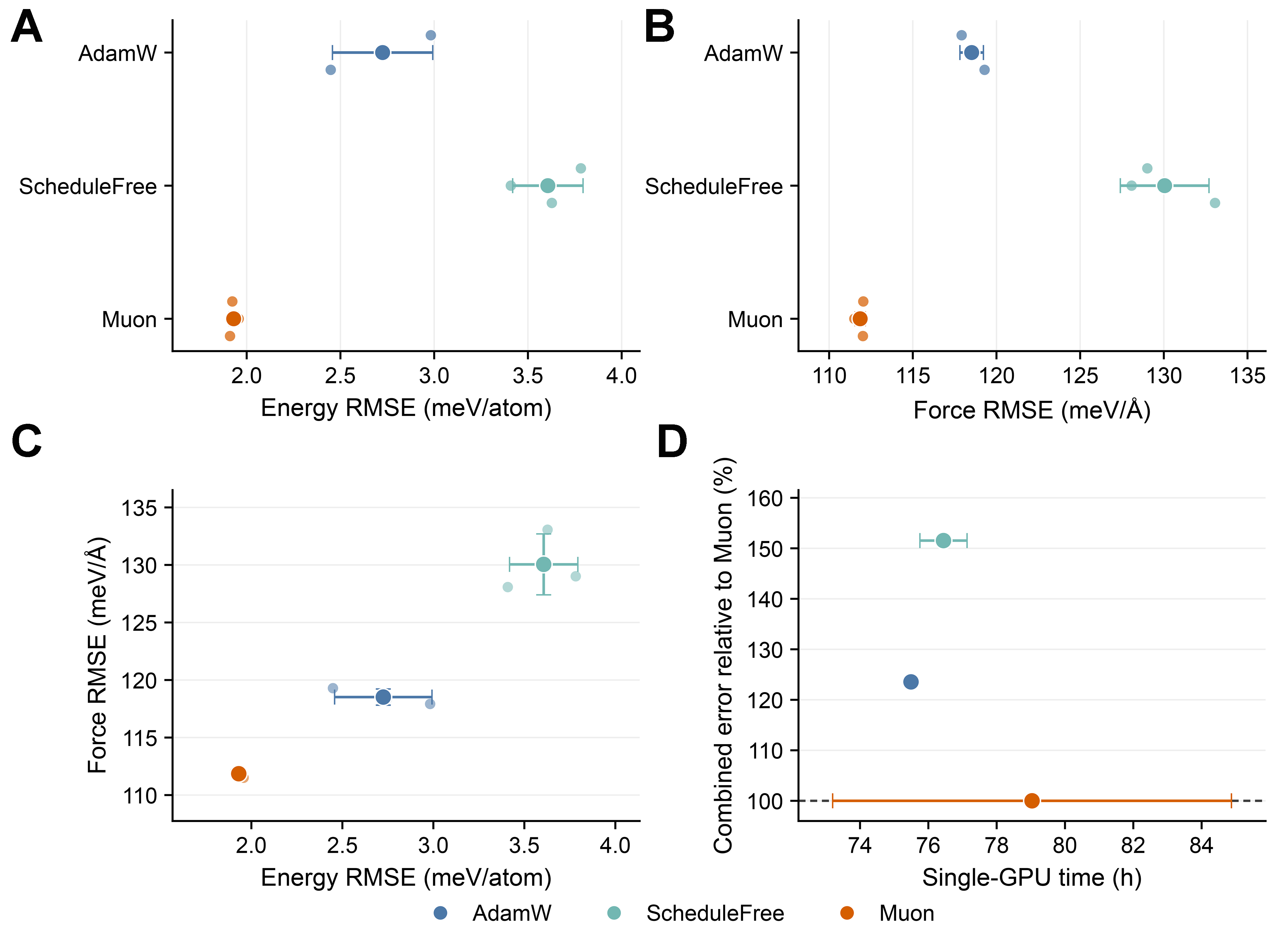
Figure 2. Fixed-subset comparison of optimizer configurations on the 200k structured MACE-OFF24 subset. (A and B) show final energy and force RMSE across three runs (points), with bars and error bars denoting mean ± sample standard deviation; (C) plots the energy–force position of each run; and (D) relates combined error to single-GPU wall-clock GPU-hours. Combined error is 100 times the mean of the energy and force RMSE ratios relative to their respective Muon means. Muon attains the lowest mean energy and force RMSEs among the three evaluated configurations. MACE: Multi-atomic cluster expansion; RMSE: root mean square error; GPU: graphics processing unit.
Fixed-subset comparison of optimizer configurations on the 200k structured subset
| Optimizer | Energy RMSE (meV/atom) | Force RMSE (meV/Å) | GPU-hours |
| Muon | 1.93 ± 0.02 (-29%) | 111.86 ± 0.30 (-6%) | 79.04 ± 5.84 |
| AdamW | 2.72 ± 0.27 | 118.52 ± 0.70 | 75.49 ± 0.11 |
| ScheduleFree | 3.61 ± 0.19 (+32%) | 130.05 ± 2.65 (+10%) | 76.44 ± 0.69 |
On the fixed subset, Muon lowers mean energy RMSE by 29.15% and force RMSE by 5.62% relative to AdamW and lowers both metrics relative to ScheduleFree. It requires 4.69% more single-graphics processing unit (GPU) time than AdamW. In a separate 25k learning-rate audit, AdamW gave lower validation energy and force RMSEs than Muon after 80 first-stage epochs. These validation results were obtained under a different protocol from that used for the three-run, 200-epoch test results in Table 1.
Table 3 compares peak memory and the first measured full-step time for the same initialized model and batch.
Cold-step GPU profile for the three optimizer configurations on the same initialized model and batch
| Optimizer | Peak allocated (GiB) | Peak reserved (GiB) | First full step (s) |
| Muon | 32.25 | 40.12 | 13.29 |
| AdamW | 32.25 | 40.12 | 6.89 |
| ScheduleFree | 32.25 | 40.12 | 14.93 |
No peak-memory difference was observed for this batch.
Figure 3 compares the historical structured, random, and stratified 49k subsets across three training runs.
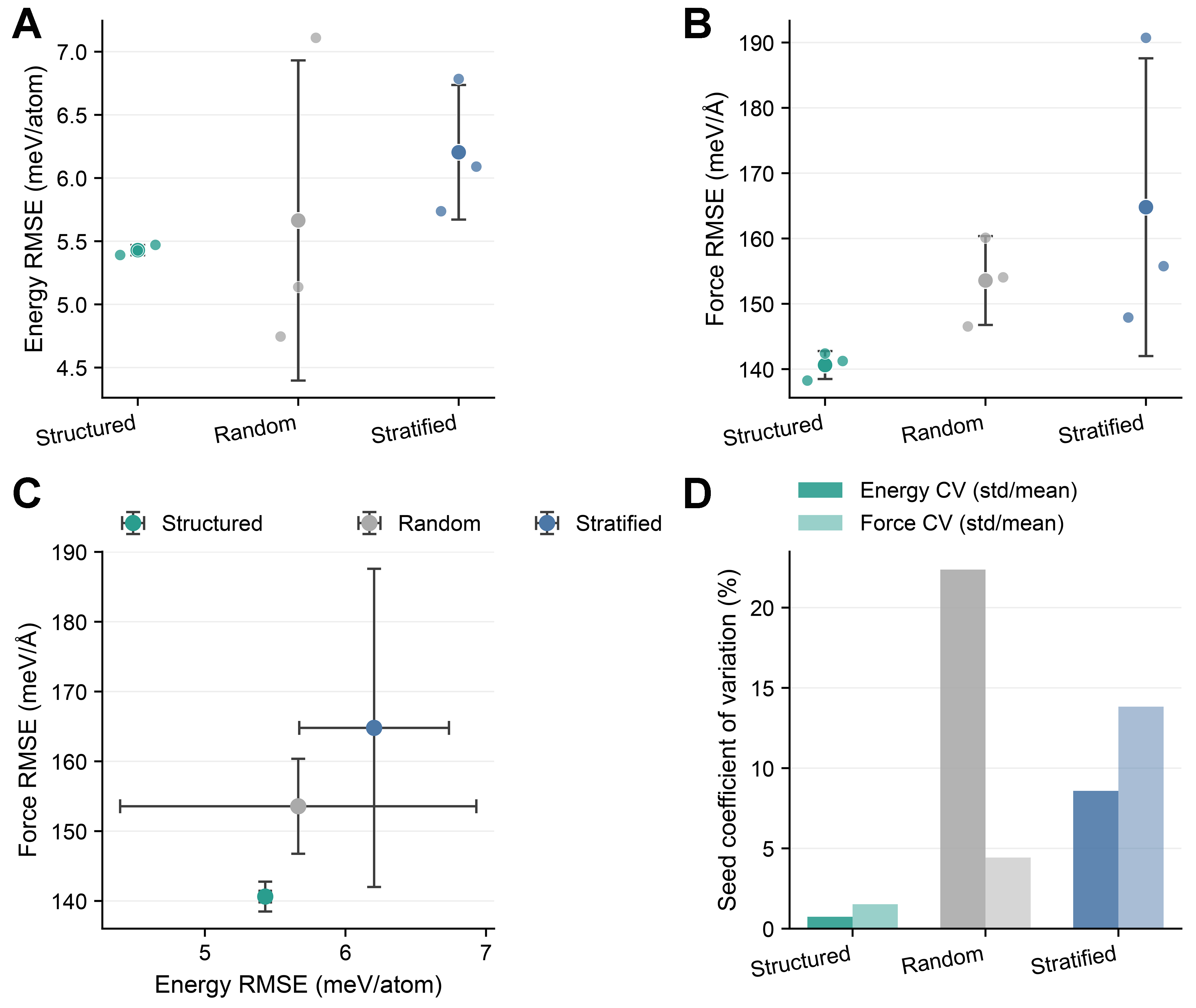
Figure 3. Configuration-selection comparison at fixed 49k selected configurations with full energy and force labels and a fixed Muon optimization protocol. Random and stratified use independently selected subsets in the three runs; structured uses one fixed historical subset. (A and B) compare energy and force RMSE across three training runs (points), with bars denoting mean ± standard deviation; (C) plots the mean energy–force positions with standard-deviation error bars; (D) reports the coefficient of variation across training runs. Structured denotes the historical pre-PCA residual/random strategy. RMSE: root mean square error; PCA: principal component analysis.
Table 4 compares five within-cluster selection rules with the pool, target size, initialization, and data-ordering settings held fixed.
Matched same-pool 49k selector comparison
| Within-cluster rule | Energy RMSE (meV/atom) | Force RMSE (meV/Å) | GPU-hours |
| Random within pool | 8.86 | 142.77 | 19.87 |
| Representative only | 5.98 | 165.85 | 18.69 |
| Residual only | 6.29 | 143.53 | 17.75 |
| Mixed 80:20 | 4.26 | 138.95 | 18.46 |
| Mixed 50:50 | 4.33 | 139.65 | 18.52 |
In this single-run comparison within the fixed label-aware pool, both mixed allocations gave lower observed energy and force RMSE than matched random sampling and either pure allocation. Relative to random within pool, the 80:20 mixture reduced energy RMSE by 51.89% and force RMSE by 2.67%; the 50:50 mixture gave closely comparable point estimates.
In a separate nine-combination candidate-pool/PCA sampling audit, subset membership changed substantially, whereas PCA explained variance and selected-residual medians remained similar; no models were retrained.
Chemical and observable structure of the remaining error
The aggregate MACE-OFF24 errors combine chemically distinct regimes into two scalars. To locate the remaining error, we examine the seven official test splits in Figure 4.
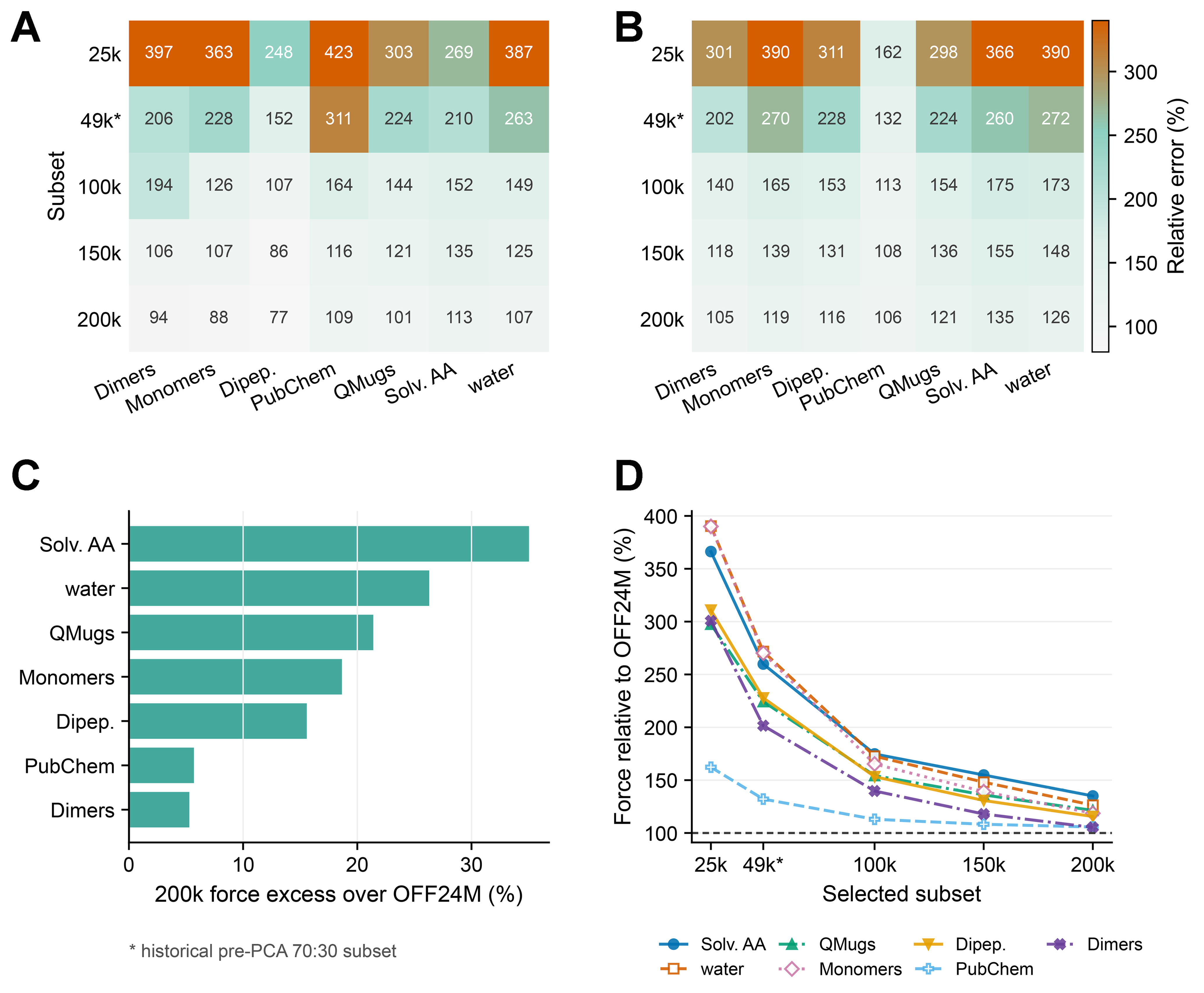
Figure 4. Split-wise MACE-OFF24 chemical-regime analysis for the target-size selection-and-training protocol. (A and B) show per-split energy and force RMSE normalized to the published full-data reference as relative RMSE percentages. A value of 100% matches the reference; only the portion exceeding 100% represents excess error; (C) reports the 200k relative force excess, 100 × (RMSE200k/RMSEreference - 1); (D) traces per-split relative force RMSE from 25k to 200k; the dashed horizontal line marks 100%. An asterisk identifies the historical pre-PCA 49k realization in (A), (B), and (D). Color, line style, marker shape, and alternating filled/open markers distinguish the seven test splits. At 200k, the largest relative force excesses occur in Solvated Amino Acids, water, and QMugs. MACE: Multi-atomic cluster expansion; RMSE: root mean square error; PCA: principal component analysis.
The split-wise pattern is not uniform. At 200k, energy RMSE is 1% above the published reference for QMugs and 6% below it for DES370K Dimers. Force RMSE is 5% above the reference for DES370K Dimers and 6% above it for PubChem. The largest relative force excesses at 200k occur in Solvated Amino Acids (35%), water (26%), and QMugs (21%). These splits include large drug-like molecules and condensed hydrogen-bonded environments whose errors are obscured by the aggregate RMSE. This pattern identifies regimes for additional coverage, force reweighting, or targeted subset construction. We next examine a chemically interpretable observable beyond the aggregate MACE-OFF24 test metrics. The 3BPA dihedral extrapolation set contains 7,047 conformers and defines a relative-energy landscape for comparing the trained models. We denote its three rotatable-bond dihedral coordinates by ϕ1, ϕ2, and ϕ3; the displayed two-dimensional slice fixes ϕ2 = 180° and varies ϕ1 and ϕ3. Each predicted landscape is anchored at the DFT-minimum conformer [Figure 5 and Table 5]. The full-landscape energy-span error is
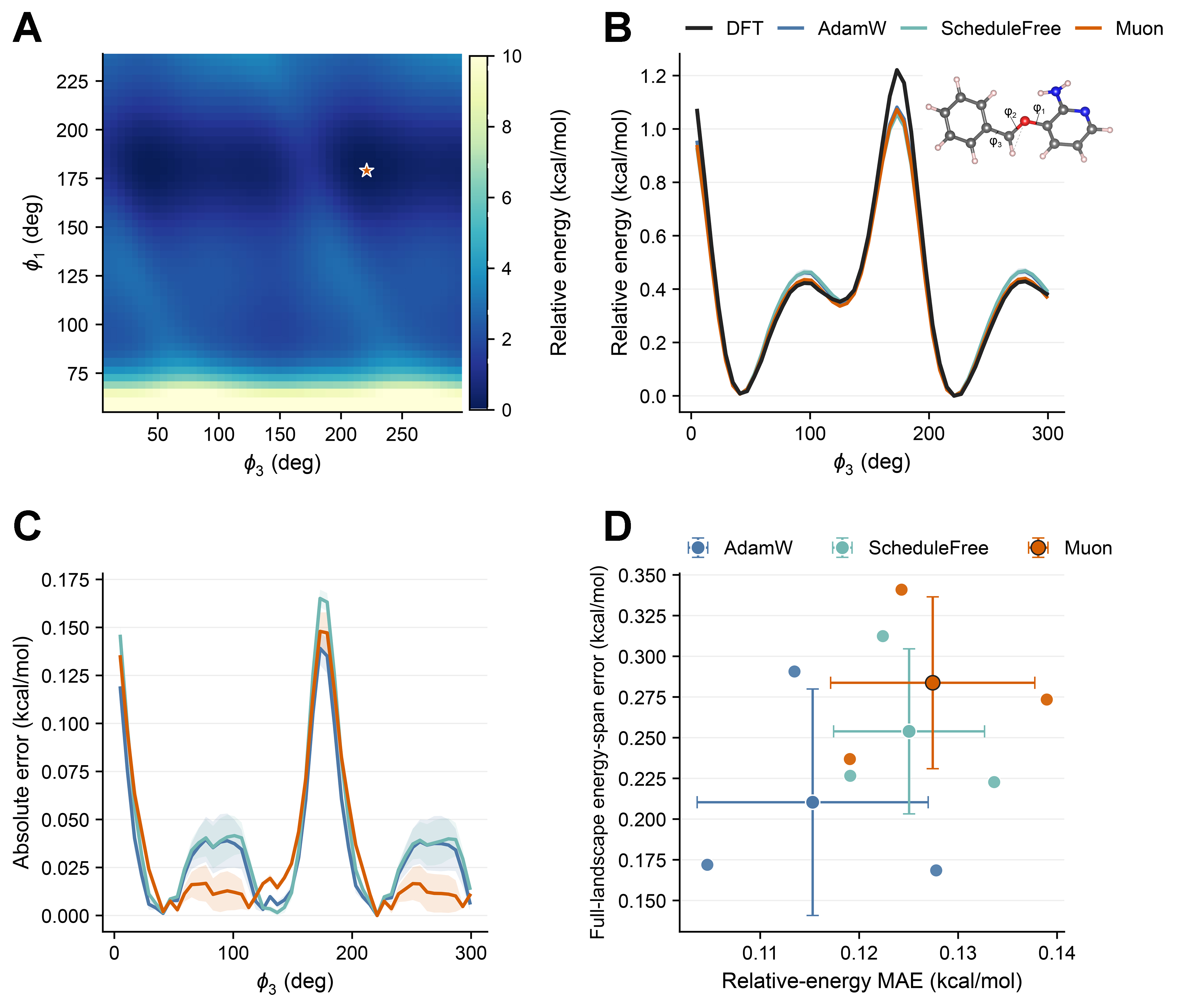
Figure 5. Conformational transfer evaluation of the optimizer configurations on the 3BPA dihedral extrapolation set (7,047 conformers). (A) shows the DFT relative-energy landscape on the ϕ2 = 180° slice, with the DFT minimum marked by a star. Values above 10 kcal/mol are shown in the color used for 10 kcal/mol; (B) compares the DFT and model-predicted profiles as ϕ3 varies through the DFT minimum at ϕ1 = 179° and ϕ2 = 180°. Its inset shows the 3BPA structure with the three torsions labeled; (C) reports the absolute errors along the same ϕ3 profile. Lines and shading in (B) and (C) denote means and standard deviations over three runs; (D) summarizes full-landscape relative-energy MAE and full-landscape energy-span error, showing individual runs and mean ± standard deviation over three runs; AdamW achieves the lowest error on both landscape metrics. Energies are reported in kcal/mol after anchoring at the DFT-minimum conformer. DFT: Density functional theory; MAE: mean absolute error.
3BPA dihedral landscape errors after anchoring at the DFT minimum
| Optimizer | Relative-energy MAE (kcal/mol) | Energy-span error (kcal/mol) |
| AdamW | 0.12 ± 0.01 | 0.21 ± 0.07 |
| ScheduleFree | 0.13 ± 0.01 | 0.25 ± 0.05 |
| Muon | 0.13 ± 0.01 | 0.28 ± 0.05 |
AdamW gives the smallest mean relative-energy MAE and full-landscape energy-span error, with lower values than Muon in all three paired runs. Muon has a more negative mean signed anchored residual (-0.09 vs. -0.06 kcal/mol) and underestimates the energy span more strongly. Post-hoc median-centering gives a mean MAE of about 0.10 kcal/mol for both optimizers. The MACE-OFF24 ranking therefore does not transfer to this relative-energy observable.
Interpretation and scope
Selecting complete configurations differs from sparse-force supervision. Our earlier work considered optimizer choice and second-order refinement during foundation-model fine-tuning[32], while Harari et al. varied force-label availability for NequIP and Allegro without removing the corresponding energy-labeled configurations[33]. Sparse-force supervision removes derivative labels from structures that remain in the data. Here, removing a configuration removes its energy and force labels as well as the chemical environment it represents.
MACE’s E(3) equivariance is architectural. Equations (8) and (9) propagate an operator-norm perturbation from the eight radial matrices to coefficients, messages, energies, and forces.
At 200k configurations, the relative force excess is largest in Solvated Amino Acids, water, and QMugs, whereas other splits are closer to the published checkpoint. This nonuniform error pattern identifies priority regimes for testing additional configurations, force weighting, or targeted selection. The teacher-residual component uses known reference energies and forces, so the reduction concerns the configurations used for subsequent model training and storage. Because Muon acts on learned parameter matrices after neighborhood construction, the same implementation can be used with periodic MACE inputs.
CONCLUSIONS
At a fixed training-set size, both configuration selection and optimizer choice affect prediction accuracy. On MACE-OFF24, our selection method combined with Muon optimization uses a selected subset comprising approximately 21% of the available configurations for training and validation. Overall energy and force RMSEs are at most 8.1% and 6% higher, respectively, than those of the published checkpoint. On the fixed 200k subset, Muon reduces mean energy and force RMSEs by 29.15% and 5.62%, respectively, compared with AdamW. In the single-run matched 49k comparison, the 80:20 mixture reduces these RMSEs by 51.89% and 2.67%, respectively, relative to same-pool random sampling under the Muon protocol. Across approximately 7,000 3BPA test conformers, AdamW instead achieves 9.52% lower mean relative-energy MAE and 25.86% lower energy-span error than Muon. The operator analysis bounds changes in predicted energies and forces under small perturbations of the radial coefficient-generator matrices. For data-efficient training, configuration selection and optimizer choice should be guided by the target chemistry and observable.
DECLARATIONS
Acknowledgments
The authors thank colleagues at the National University of Singapore and Shanghai Jiao Tong University for helpful discussions. National University of Singapore Information Technology provided computational resources.
Authors’ contributions
Conception and design of the study: Liu, X.; Wang, Y.; Shen, L.
Data acquisition, computational investigation, formal analysis, visualization, and preparation of the original draft: Liu, X.
Methodology and mathematical analysis: Liu, X.; Wang, Y.
Supervision and critical revision of the manuscript: Wang, Y.; Shen, L.
Funding acquisition and project administration: Shen, L.
All authors reviewed and approved the final manuscript.
Availability of data and materials
The molecular benchmark is available from the Cambridge repository (https://doi.org/10.17863/CAM.107498); the 3BPA source is available at https://doi.org/10.1021/acs.jctc.1c00647. Code and configurations are available in Muon-MACE (https://github.com/ShiQiaoL/Muon-MACE/), and selection data and results are in the associated Hugging Face repository (https://huggingface.co/datasets/shiqiao123/Muon-MACE-data). Released teacher data contain residuals, not complete predictions. The original teacher identity and complete 3BPA fine-tuning configurations remain unrecovered.
AI and AI-assisted tools statement
During manuscript preparation, OpenAI Codex was used with GPT-5.6 Sol (released 2026-07-09) for the original submission and GPT-6 Astra (released 2026-09-03) for revision and responses to reviewers. The tools assisted with language editing, manuscript formatting, code checking, and figure preparation. The authors directed the study design, data collection, analysis, and interpretation, and reviewed and verified all AI-assisted outputs. All authors take full responsibility for the accuracy, integrity, and final content of the manuscript.
Financial support and sponsorship
This research was supported under grant CFP04-CF-019. Lei Shen acknowledges financial support from the Singapore Ministry of Education Tier 2 (A-8001872-00-00). The funders had no role in the study design, data analysis and interpretation, or preparation of the manuscript.
Conflicts of interest
Shen, L. is an Associate Editor of the Journal of Materials Informatics and was not involved in the editorial processing of this manuscript. The other authors declared that there are no conflicts of interest.
Ethical approval and consent to participate
Not applicable.
Consent for publication
Not applicable.
Copyright
©The Author(s) 2026.
REFERENCES
1. Behler, J.; Parrinello, M. Generalized neural-network representation of high-dimensional potential-energy surfaces. Phys. Rev. Lett. 2007, 98, 146401.
2. Bartók, A. P.; Payne, M. C.; Kondor, R.; Csányi, G. Gaussian approximation potentials: the accuracy of quantum mechanics, without the electrons. Phys. Rev. Lett. 2010, 104, 136403.
3. Shapeev, A. V. Moment tensor potentials: a class of systematically improvable interatomic potentials. Multiscale. Model. Simul. 2016, 14, 1153-73.
4. Smith, J. S.; Isayev, O.; Roitberg, A. E. ANI-1: an extensible neural network potential with DFT accuracy at force field computational cost. Chem. Sci. 2017, 8, 3192-203.
5. Chmiela, S.; Tkatchenko, A.; Sauceda, H. E.; Poltavsky, I.; Schütt, K. T.; Müller, K. Machine learning of accurate energy-conserving molecular force fields. Sci. Adv. 2017, 3, e1603015.
6. Zhang, L.; Han, J.; Wang, H.; Car, R.; E, W. Deep potential molecular dynamics: a scalable model with the accuracy of quantum mechanics. Phys. Rev. Lett. 2018, 120, 143001.
7. Unke, O. T.; Meuwly, M. PhysNet: a neural network for predicting energies, forces, dipole moments, and partial charges. J. Chem. Theory. Comput. 2019, 15, 3678-93.
8. Behler, J. Perspective: Machine learning potentials for atomistic simulations. J. Chem. Phys. 2016, 145, 170901.
9. Unke, O. T.; Chmiela, S.; Sauceda, H. E.; et al. Machine learning force fields. Chem. Rev. 2021, 121, 10142-86.
10. Ko, T. W.; Ong, S. P. Recent advances and outstanding challenges for machine learning interatomic potentials. Nat. Comput. Sci. 2023, 3, 998-1000.
11. Batzner, S.; Musaelian, A.; Sun, L.; et al. E(3)-equivariant graph neural networks for data-efficient and accurate interatomic potentials. Nat. Commun. 2022, 13, 2453.
12. Musaelian, A.; Batzner, S.; Johansson, A.; et al. Learning local equivariant representations for large-scale atomistic dynamics. Nat. Commun. 2023, 14, 579.
13. Chen, C.; Ong, S. P. A universal graph deep learning interatomic potential for the periodic table. Nat. Comput. Sci. 2022, 2, 718-28.
14. Deng, B.; Zhong, P.; Jun, K.; et al. CHGNet as a pretrained universal neural network potential for charge-informed atomistic modelling. Nat. Mach. Intell. 2023, 5, 1031-41.
15. Merchant, A.; Batzner, S.; Schoenholz, S. S.; Aykol, M.; Cheon, G.; Cubuk, E. D. Scaling deep learning for materials discovery. Nature 2023, 624, 80-5.
16. Yang, H.; Hu, C.; Zhou, Y.; et al. MatterSim: a deep learning atomistic model across elements, temperatures and pressures. arXiv 2024, arXiv:2405.04967. Available online: https://doi.org/10.48550/arXiv.2405.04967. (accessed 2026-10-12).
17. Zhang, D.; Peng, A.; Cai, C.; et al. A graph neural network for the era of large atomistic models. npj. Comput. Mater. 2026, 12, 276.
18. Yuan, E. C. Y.; Liu, Y.; Chen, J.; et al. Foundation models for atomistic simulation of chemistry and materials. Nat. Rev. Chem. 2026, 10, 212-30.
19. Li, Y.; Zhang, X.; Liu, M.; Shen, L. A critical review of machine learning interatomic potentials and Hamiltonian. J. Mater. Inf. 2025, 5, 43.
20. Podryabinkin, E. V.; Shapeev, A. V. Active learning of linearly parametrized interatomic potentials. Comput. Mater. Sci. 2017, 140, 171-80.
21. Podryabinkin, E. V.; Tikhonov, E. V.; Shapeev, A. V.; Oganov, A. R. Accelerating crystal structure prediction by machine-learning interatomic potentials with active learning. Phys. Rev. B. 2019, 99, 064114.
22. Zhang, L.; Lin, D. Y.; Wang, H.; Car, R.; E, W. Active learning of uniformly accurate interatomic potentials for materials simulation. Phys. Rev. Mater. 2019, 3, 023804.
23. Zhang, Y.; Wang, H.; Chen, W.; et al. DP-GEN: a concurrent learning platform for the generation of reliable deep learning based potential energy models. Comput. Phys. Commun. 2020, 253, 107206.
24. Vandermause, J.; Torrisi, S. B.; Batzner, S.; et al. On-the-fly active learning of interpretable Bayesian force fields for atomistic rare events. npj. Comput. Mater. 2020, 6, 20.
25. Lookman, T.; Balachandran, P. V.; Xue, D.; Yuan, R. Active learning in materials science with emphasis on adaptive sampling using uncertainties for targeted design. npj. Comput. Mater. 2019, 5, 21.
26. Zaverkin, V.; Holzmüller, D.; Steinwart, I.; Kästner, J. Exploring chemical and conformational spaces by batch mode deep active learning. Digit. Discov. 2022, 1, 605-20.
27. David, R.; de la Puente, M.; Gomez, A.; Anton, O.; Stirnemann, G.; Laage, D. ArcaNN: automated enhanced sampling generation of training sets for chemically reactive machine learning interatomic potentials. Digit. Discov. 2025, 4, 54-72.
28. Andolina, C. M.; Saidi, W. A. Highly transferable atomistic machine-learning potentials from curated and compact datasets across the periodic table. Digit. Discov. 2023, 2, 1070-7.
29. Liu, Y.; He, X.; Mo, Y. Discrepancies and error evaluation metrics for machine learning interatomic potentials. npj. Comput. Mater. 2023, 9, 174.
30. Zou, J.; Marzouk, Y. Data curation for machine learning interatomic potentials by determinantal point processes. arXiv 2026, arXiv:2603.22160. Available online: https://doi.org/10.48550/arXiv.2603.22160. (accessed 2026-10-12).
31. Baghishov, I.; Janssen, J.; Henkelman, G.; Perez, D. Application-specific machine-learned interatomic potentials: exploring the trade-off between DFT convergence, MLIP expressivity, and computational cost. Digit. Discov. 2026, 5, 332-47.
32. Liu, X.; Wang, Y.; Zhao, T. Beyond Adam: disentangling optimizer effects in the fine-tuning of atomistic foundation models. AI. Sci. 2026, 2, 015004.
33. Harari, G.; Zimmermann, Y.; Kulseng, O. T.; et al. Beyond Adam: SOAP and Muon for faster, label-efficient training of machine learning interatomic potentials. arXiv 2026, arXiv:2607.02499. Available online: https://doi.org/10.48550/arXiv.2607.02499. (accessed 2026-10-12).
34. Stupariu, T. M.; Manolache, A. How the optimizer shapes learned solutions in equivariant neural networks. arXiv 2026, arXiv:2605.27662. Available online: https://doi.org/10.48550/arXiv.2605.27662. (accessed 2026-10-12).
35. Zhang, H. PolarAdamW: disentangling spectral control and schur gauge-equivariance in matrix optimisation. arXiv 2026, arXiv:2605.07067. Available online: https://doi.org/10.48550/arXiv.2605.07067. (accessed 2026-10-12).
36. Kovács, D. P.; Moore, J. H.; Browning, N. J.; et al. MACE-OFF: short-range transferable machine learning force fields for organic molecules. J. Am. Chem. Soc. 2025, 147, 17598-611.
37. Batatia, I.; Kovacs, D. P.; Simm, G. N. C.; Ortner, C.; Csanyi, G. MACE: higher order equivariant message passing neural networks for fast and accurate force fields. Adv. Neural Inf. Process. Syst. 2022, 35, 11423-36.
38. Jordan, K.; Jin, Y.; Boza, V.; et al. Muon: an optimizer for hidden layers in neural networks. 2024. https://kellerjordan.github.io/posts/muon/. (accessed 2026-10-12).
39. Loshchilov, I.; Hutter, F. Decoupled weight decay regularization. In International Conference on Learning Representations (ICLR); 2019. https://openreview.net/forum?id=Bkg6RiCqY7. (accessed 2026-10-12).
40. Defazio, A.; Yang, X. A.; Mehta, H.; Mishchenko, K.; Khaled, A.; Cutkosky, A. The road less scheduled. Adv. Neural Inf. Process. Syst. 2024, 37, 9974-10007.
41. Higham, N. J. Functions of matrices: theory and computation. Society for Industrial and Applied Mathematics; 2008.
Cite This Article
 Open Access
How to Cite
Liu, X.; Wang, Y.; Shen, L. Configuration selection and matrix-aware optimization for data-efficient atomistic foundation models. J. Mater. Inf. 2026, 6, 57. https://dx.doi.org/10.20517/jmi.2026.62
Download Citation
If you have the appropriate software installed, you can download article citation data to the citation manager of your choice. Simply select your manager software from the list below and click on download.
Export Citation File
Type of Import
Tips on Downloading Citation
Citation Manager File Format
Type of Import
Direct Import: When the Direct Import option is selected (the default state), a dialogue box will give you the option to Save or Open the downloaded citation data. Choosing Open will either launch your citation manager or give you a choice of applications with which to use the metadata. The Save option saves the file locally for later use.
Indirect Import: When the Indirect Import option is selected, the metadata is displayed and may be copied and pasted as needed.
About This Article
Copyright

Data & Comments
Data
0











Comments
Comments must be written in English. Spam, offensive content, impersonation, and private information will not be permitted. If any comment is reported and identified as inappropriate content by OAE staff, the comment will be removed without notice. If you have any queries or need any help, please contact us at [email protected].