

Integrating physical metallurgy principles and machine learning for predicting continuous cooling phase transformations in steel
 0
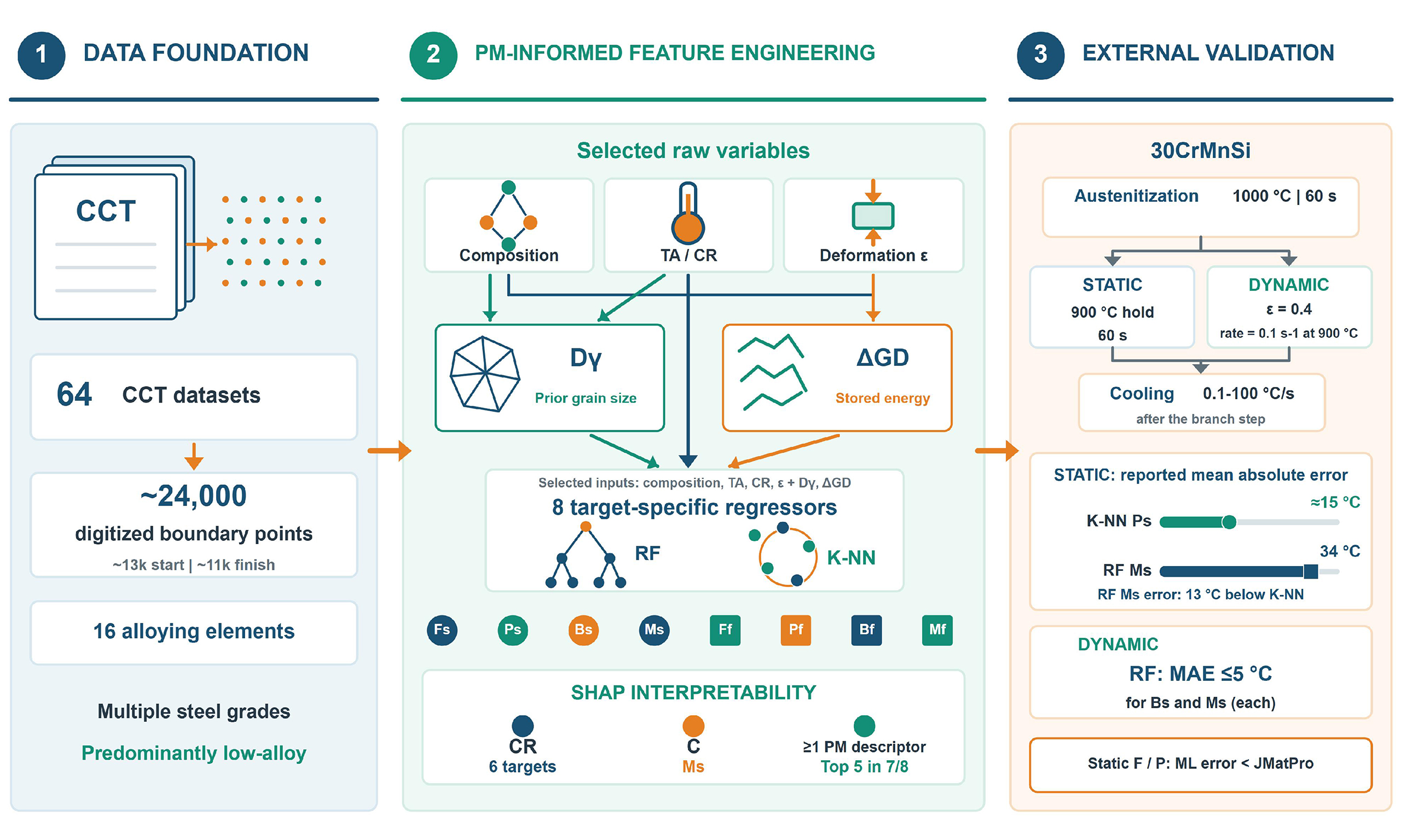
0 Graphical Abstract
Abstract
This study presents a high-precision predictive model for continuous cooling transformation (CCT) behavior in steel by integrating physical metallurgy (PM) principles with machine learning (ML) methods. To enhance industrial applicability, thermal deformation parameters are incorporated alongside chemical composition and cooling conditions. Supplementary features, including dislocation energy (ΔGD) and austenite grain size (Dγ) calculated from PM models, further strengthen the predictive capability. The dataset comprises 64 sets of CCT curves from multiple steel grades. Random forest (RF) and K-nearest neighbor (K-NN) algorithms are used to predict eight key phase transformation temperatures in steels. Model accuracy was validated using both static and dynamic dilatation experiments on 30CrMnSi steel. Evaluated on the internally random-split test subset, the optimized RF and K-NN models achieve a coefficient of determination (R2) at or above 0.99 for most phase transformation temperatures, with mean absolute error (MAE) mostly within 3.0 °C. Exceptions include Ps for the RF model, Ps and Pf for the K-NN model. SHapley Additive exPlanations analysis identifies cooling rate and carbon content as the most influential factors, with PM-derived parameters also playing significant roles. The model performance was further assessed via static and dynamic dilatation experiments on 30CrMnSi steel. Both models accurately capture the rise in transformation temperature and the leftward shift of the CCT curve resulting from deformation. These PM-driven ML models provides an accurate and interpretable tool for predicting static and dynamic CCT curves, supporting intelligent design and process optimization of high-performance steels.
Keywords


 Download PDF
INTRODUCTION
Amid the national “carbon neutrality” strategy, the steel industry faces inherent conflicts among resource allocation, environmental protection, and production capacity. Traditional research and development primarily relied on experimental trial-and-error methods. Extensive microstructure and property testing yields low efficiency[1,2] and escalates costs. There is an urgent demand for an innovative production research model to enhance efficiency and support low-carbon, intelligent production[3-5]. Steel properties largely depend on its chemical composition and microstructure, determined by phase transformation dynamics during processing. Continuous cooling transformation (CCT) curves serve as a foundational tool for analyzing phase transformations and optimizing heat treatment[6]. Standard methods for determining CCT curves, such as metallographic hardness testing and expansion testing[7], are laborious, expensive, and require advanced expertise[8]. These constraints impede efficient development for the next generation of high-performance steel.
The integration of artificial intelligence and big data technologies is fundamentally transforming the landscape of materials research and development. Traditional trial-and-error methods and empirical experience are shifting towards a data- and algorithm-driven mode underpinned by Materials Informatics. As a cost-effective, efficient, and expedient data-driven approach, machine learning (ML) offers a novel paradigm for materials science. ML can extract complex patterns from existing experimental data, enabling accurate prediction of target properties[9,10]. Currently, ML has been widely adopted in the steel industry[11,12].
Numerous researchers have leveraged ML models to achieve quantitative predictions of CCT diagrams in steels. Table 1 provides an overview of both domestic and international studies employing ML approaches to predict phase transformation temperatures in steels.
Summary of ML models for predicting phase transformation temperatures
| Target | Algorithm | Database input | Database source | Alloy | Ref. |
| Fs, Bs, Ms, Hardness | K-NN, RC, RF, MLPreg | Compositions, cooling rate | NIMS Materials Database | Ni-Cr-Mo steel | [13] |
| Ac3, Fs, Ps, Bs, Ms | RF, MR, SVR, XGBoost | Compositions | NRIM Atlas 1 | Structural steel | [14] |
| Fs, Ps, Bs, Ms, Pf, Hardness | MLPReg, SVR, RF, RBFReg, K-NN | Compositions, cooling rate | Japan National Institute of Material Science database | Low-alloy steel | [15] |
| Fs, Ps, Bs, Ms | The BP and RBF neural networks | Compositions, transformation time, Ac1, cooling rate | NIMS Materials Database | Steels | [16] |
| Ms | RF, ExT, GB, AdB | Compositions | Literature | Steels | [17] |
| Bs | RFR, ANN, K-NN | Compositions, austenite average grain size | Literature | Low-alloy steel | [18] |
| Ms | RFR, SVR, K-NN | Compositions, austenite average grain size | Literature | Alloy steel | [19] |
| Ms, Bs, Ac1, Ac3 | LightGBM | Compositions, heating rate, cooling rate, atomic parameters | Materials Algorithms Project | Steels | [20] |
| Fs, Ff, Ps, Pf, Bs, Bf | MLP, GRNN | Compositions, cooling rate, TA | Literature | Structural steel, machinable steel | [21] |
| Ac1, Ac3, Fs, Ps, Bs, Ms, tF, tB, tP | MLP | Compositions, cooling rate, TA | Literature | Engineering steel, structural steels | [22] |
| Ac1, Ac3, Fs, Ps, Bs, Ms, Ff, Pf, Bf, Hardness | ANN | Compositions, cooling rate, TA | Literature | Structural steel, engineering steel | [23] |
| Fs, Ps, Bs, Ff, Pf, Bf, | ANN | Compositions, cooling rate, TA | Literature | Low-carbon steel | [24,25] |
| Ps, Pf, Bs, Bf, Ms | MLPReg, K-NN, Bagging, RF | Compositions, cooling rate, TA | Literature | Tool steel | [7] |
Despite significant advances, deformation parameters have rarely been incorporated into ML models for CCT prediction[26]. In practical steel production, however, deformation is a critical process for developing high-performance materials, as it plays a key role in microstructure refinement and property enhancement[27,28]. Moreover, incorporating physical metallurgy (PM) knowledge into ML frameworks is increasingly recognized as an effective strategy for guiding feature engineering, thereby improving the credibility and predictive accuracy of such models.
For instance, Li et al. utilized CALPHAD calculations to generate phase constitution and microstructural targets, which were then employed to construct or constrain ML mappings[29]. This approach facilitated a data-driven co-design of alloy composition, processing parameters, and microstructure. Song et al. demonstrated that a PM-constrained ML approach can accurately predict stacking fault energy in austenitic stainless steel, underscoring the value of integrating physical priors[30]. Therefore, combining these two strategies is anticipated to further improve the applicability of ML models for phase transformation prediction and support the development of advanced steel grades.
Recent research efforts have increasingly focused on incorporating the effects of deformation into the ML framework. For instance, Cao et al. proposed a PM-guided hereditary ML method for HSLA steels, utilizing theoretical models to calculate austenite grain size and deformation-stored energy as input features[8]. This approach significantly enhanced prediction accuracy. Additionally, in studies targeting specific process scenarios such as welding and hot stamping, macroscopic process parameters, including strain and strain rate, have been introduced to effectively characterize the influence of deformation[31]. Consideration of deformation factors is crucial for accurate phase transformation modeling. Nonetheless, current approaches remain limited in both the physical depth of input features and model generalizability. Many methods rely on macroscopic process parameters, which do not fully reflect the underlying microstructural mechanisms of deformation. Alternatively, models incorporating microstructural physical parameters are often developed for specific steel grades, constraining applicability across a broader range of materials.
To overcome current limitations, this study proposes a PM-guided ML framework for predicting static and dynamic CCT curves with three distinctive contributions. First, in contrast to the work of Cao et al.[8], which focused on HSLA steels, the applicability of PM state parameters is extended to a wider array of steels by introducing two physically derived descriptors, dislocation energy (ΔGD) and austenite grain size (Dγ), as supplementary input features, thereby enhancing physical consistency and compositional generalizability. The ΔGD originates from hotdeformation, whereas Dγ describes the prioraustenite grain size before deformation and is governed by alloy composition together with austenitization conditions. Both descriptors are linked to the driving force for phase transformation and regulation of nucleation sites and rates. Second, a comprehensive database of approximately 24,000 data points was constructed from systematically collected literature data covering a broad compositional range and a wide spectrum of cooling rates, including deformation parameters that are rarely incorporated in existing datasets. Third, SHapley Additive exPlanations (SHAP) analysis is employed to provide systematic model interpretability, quantifying the contribution of PM-derived features and confirming qualitative consistency with established metallurgical principles. Using this dataset, Random forest (RF) and K-nearest neighbor (K-NN) algorithms were trained and optimized to predict transformation temperatures at specified cooling rates, from which CCT diagrams can be reconstructed, and accuracy was validated against experimental static and dynamic CCT curves of 30CrMnSi steel. This work thus provides an accurate, interpretable, and industrially relevant tool for advancing steel production through intelligent process design.
MATERIALS AND METHODS
Data collection and feature engineering
This study systematically reviewed published literature on steel CCT diagrams from the past two decades, covering a wide range of steel grades. To ensure data reliability, the initial screening prioritized sources providing comprehensive experimental parameters, including chemical composition, austenitizing temperature and time, deformation conditions, and metallographic verification of microstructure. Key phase transformation points were then extracted from the reported CCT curves using the image digitization tool in Origin software.
The data extraction process is as follows: temperature units were standardized to Celsius, time units to seconds, and the time axis was converted to a logarithmic scale, log(t). Original curve images were imported into the software, where horizontal and vertical coordinate ranges were manually defined, and the coordinate system was mapped using the origin and the points of maximum temperature and time. The start and finish temperatures of each phase transformation, along with their corresponding times (t), were then systematically extracted point-by-point from the CCT curves using the sampling method shown in Figure 1. Data points that were ambiguous in phase-transformation inflection identification or showed abrupt temperature jumps inconsistent with the local digitization/readout from the same source (i.e., apparent digitization or tracing artifacts) were excluded standard data-validation practice for curated experimental/digitized materials data. Genuine, physically meaningful non-monotonic behavior was retained. The screened dataset preserves the original experimental variability while removing only clear extraction errors to avoid spurious interference in subsequent ML models. The digitization process inevitably introduces reading errors associated with image resolution and coordinate mapping. Based on repeated extractions of selected CCT curves, the estimated uncertainty in transformation temperatures is within
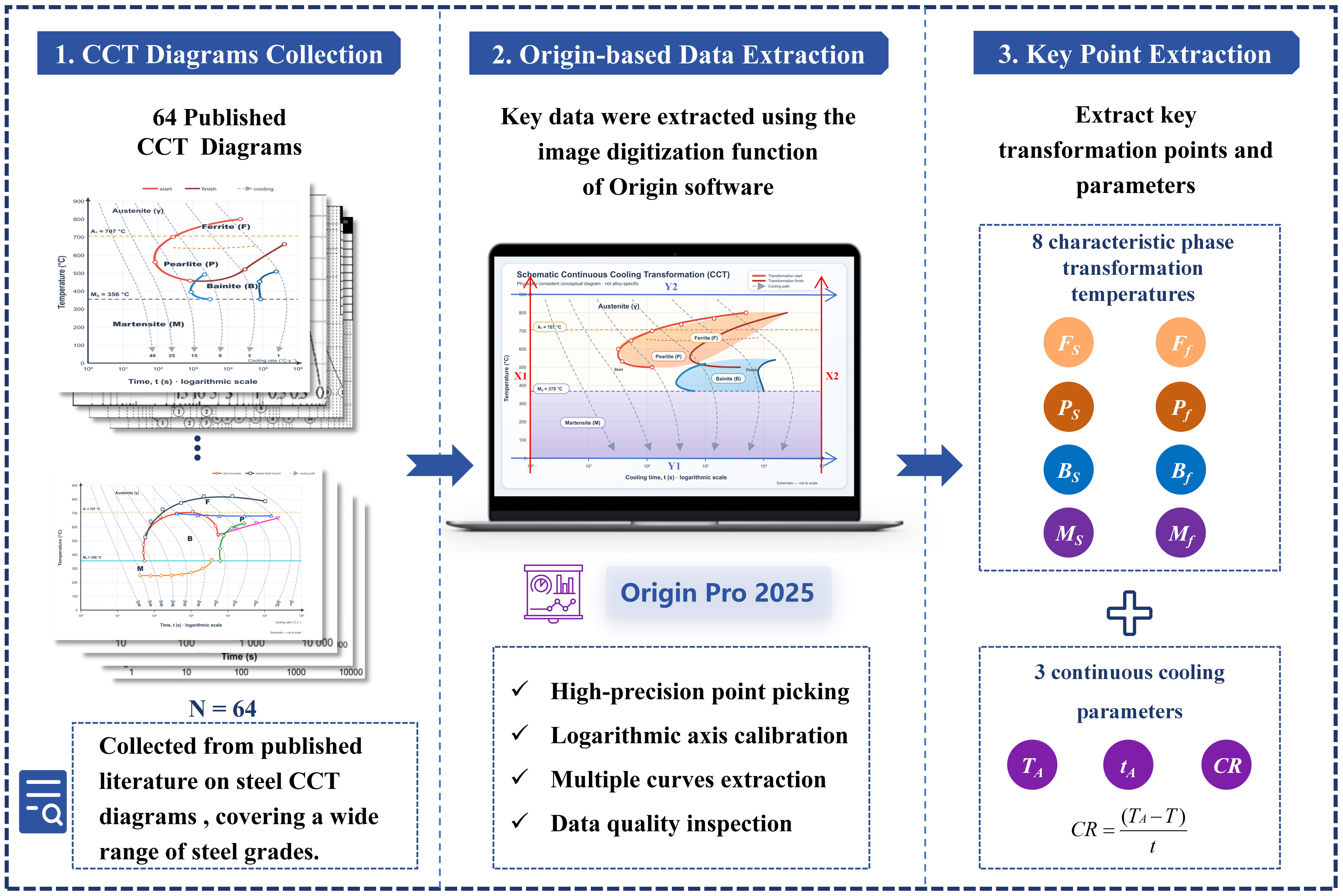
Figure 1. Data points extracted from the CCT diagrams using an image digitization tool. CCT: Continuous cooling transformation; Fs: ferrite transformation start temperature; Ff: ferrite transformation finish temperature; Ps: pearlite transformation start temperature; Pf: pearlite transformation finish temperature; Bs: bainite transformation start temperature; Bf: bainite transformation finish temperature; Ms: martensite transformation start temperature; Mf: martensite transformation finish temperature; TA: austenitizing temperature; tA: austenitizing time; CR: cooling rate.
Finally, all data were consolidated into an Excel spreadsheet to establish a comprehensive database. The database fields include 16 chemical elements (C, Si, Mn, Ni, Cr, Mo, V, Al, Ti, Nb, B, P, S, Cu, W, N); 8 phase transformation temperatures (Fs, Ff; Ps, Pf; Bs, Bf; Ms, Mf); 3 continuous cooling parameters (austenitizing temperature TA, austenitizing time tA, cooling rate CR); and 3 deformation process parameters (deformation amount ε, deformation temperature Tε, deformation rate
To account for the effect of deformation on phase transformation kinetics, two key supplementary input features were calculated based on PM principles: dislocation energy ΔGD and austenite grain size Dγ.
Calculation of ΔGD begins by determining the flow stress (σ) through the Arrhenius model [Equation (1)], which links deformation parameters with material properties. The material constants A, β, and n are obtained using the model by Hatta et al.[32], and the carbon content of the material, while the deformation activation energy Q is evaluated according to the model developed by Medina et al. and the chemical composition[33]. Once the flow stress σ is obtained, it is substituted into Equation (2) to calculate ΔGD.
where the Taylor factor M is 3.11 [for face-centered cubic (FCC) metals], the shear modulus G is 79 GPa (representing austenitic shear modulus), and the constant α is 0.15 (for FCC metals)[8,34]. It should be noted that Equation (2) directly yields the dislocation stored energy per unit volume with dimensions of J/m3. In this work, we report the ΔGD values in kJ/m3 to keep the numerical range convenient for subsequent ML processing.
For Dγ, the austenite grain size, the model proposed by Wang et al. is adopted[35]. This model calculates grain size from material composition and austenitizing parameters, as given in[35]:
where the chemical composition (in wt.%), austenitizing temperature TA, and austenitizing time tA are sourced from the database, and R is the universal gas constant, typically taken as 8.314 J/(mol·K). Notably, the obtained Dγ represents the prior-austenite grain size before hot deformation; grain-refinement effects induced by deformation are not incorporated here and are instead characterized by ΔGD. The successful construction of two supplementary PM input features enhances the interpretability and rationality of the ML model.
A total of 64 sets of steel CCT curve data were collected, yielding nearly 13,000 data points for phase transformation start temperatures and almost 11,000 data points for finish temperatures. Model inputs include 16 elemental compositions, austenitizing temperature TA, cooling rate CR, deformation amount ε, as well as two computationally derived PM parameters ΔGD and Dγ. The raw parameters tA, Tε, and
Statistical analysis of data distribution in the database
| Data type | Characteristic | Minimum | Maximum | Mean | Standard deviation |
| Inputs | C (wt%) | 0.09 | 0.84 | 0.291 | 0.157 |
| Si (wt%) | 0 | 1.46 | 0.440 | 0.373 | |
| Mn (wt%) | 0.25 | 2.96 | 1.238 | 0.506 | |
| Ni (wt%) | 0 | 2.5 | 0.168 | 0.431 | |
| Cr (wt%) | 0 | 1.31 | 0.438 | 0.459 | |
| Mo (wt%) | 0 | 0.72 | 0.100 | 0.133 | |
| V (wt%) | 0 | 0.25 | 0.019 | 0.051 | |
| Al (wt%) | 0 | 1.37 | 0.023 | 0.114 | |
| Ti (wt%) | 0 | 0.04 | 0.011 | 0.015 | |
| Nb (wt%) | 0 | 0.034 | 0.006 | 0.013 | |
| B (wt%) | 0 | 0.003 | 0.001 | 0.001 | |
| P (wt%) | 0 | 0.081 | 0.012 | 0.013 | |
| S (wt%) | 0 | 0.06 | 0.009 | 0.012 | |
| Cu (wt%) | 0 | 0.32 | 0.024 | 0.066 | |
| W (wt%) | 0 | 2.25 | 0.032 | 0.267 | |
| N (wt%) | 0 | 0.0093 | 0.001 | 0.002 | |
| TA (°C) | 725 | 1,200 | 897.227 | 69.552 | |
| CR (°C/s) | 0.003 | 638.297 | 23.753 | 54.141 | |
| ε | 0 | 1 | 0.203 | 0.271 | |
| Dγ (μm) | 0.017 | 26.573 | 1.974 | 3.673 | |
| ΔGD (kJ/m3) | 0 | 29,447.966 | 5,504.648 | 7,472.917 | |
| Outputs Outputs | Fs (°C) | 434.449 | 873.592 | 708.388 | 74.001 |
| Ps (°C) | 454.618 | 766.238 | 655.172 | 49.769 | |
| Bs (°C) | 332.307 | 725.714 | 535.785 | 61.109 | |
| Ms (°C) | 107.657 | 553.053 | 342.561 | 62.964 | |
| Ff (°C) | 382.706 | 755.802 | 611.549 | 70.444 | |
| Pf (°C) | 290.971 | 725.714 | 580.434 | 61.957 | |
| Bf (°C) | 108.160 | 708.999 | 369.811 | 61.745 | |
| Mf (°C) | 76.554 | 381.070 | 222.961 | 56.565 |
As shown in Table 2 and Supplementary Figure 1, the database covers a carbon content range of 0.09-0.84 wt.%, capturing both low-carbon and high-carbon steels. Alloying elements such as Si, Mn, and Cr exhibit a broad distribution, and the cooling rate range spans from 0.003 to over 600 °C/s, demonstrating strong data representativeness. The database is primarily composed of low-alloy steel data, providing relatively comprehensive material information, although data on high-alloy compositions are relatively sparse.
Although this sparsity may affect the accuracy of predictions for certain alloys, it increases the scalability and generalization of the model across a wider compositional space. In contrast to most existing CCT prediction ML models, which typically focus on static heat-treatment conditions and are limited to low-alloy steels or specific grades[36], this database extends coverage to high-carbon and complex high-alloy systems, improving model universality. Furthermore, by incorporating actual hot-deformation parameters, such as deformation amount and deformation temperature, the database supports the development of a dynamic phase transformation prediction model tailored to the hot-rolling process.
Additional descriptions of dataset visualization, featurescreening procedures, hyperparameter optimization, and model performance metrics are provided in Supplementary Materials.
Data preprocessing and feature selection
High-quality data forms the basis for building accurate and reliable ML models. Systematic preprocessing and feature selection of raw data prior to model training can effectively improve predictive performance and generalization. In this study, Python toolkits such as NumPy, Pandas, and Matplotlib were used for data preprocessing, including data cleaning, handling missing values, outlier removal, data standardization, and feature correlation analysis. These steps establish a robust foundation for developing a high-precision steel CCT curve prediction model.
The constructed steel CCT curve database contains multidimensional features, several of which include missing values, outliers, and duplicate samples that must be addressed before modeling. Missing values not critical to phase transformation were interpolated, while others, along with anomalous and duplicate samples, were removed. To standardize inputs for K-NN modeling, Z-score normalization was applied, ensuring a mean of 0 and a standard deviation of 1, as given in:
where x is the raw data, μ is the mean, σ is the standard deviation, and Z is the standardized data.
To reduce model complexity and improve computational efficiency, input features were filtered prior to modeling. The Pearson correlation coefficient was used to assess the linear relationship between each feature and the target phase transformation temperature, as given in:
where xi and yi are the feature values, and
ML modeling
RF and K-NN are selected in this work. On one hand, the ensemble-based RF features favorable modeling stability and enables interpretable feature quantification via SHAP analysis, which well accommodates the nonlinear phase transformation behavior coupled with PM parameters. On the other hand, K-NN follows a straightforward principle without explicit function fitting. The two algorithms with distinct modeling mechanisms can be cross-compared to objectively verify the reliability of the established database and input feature system. Using the optimized database, RF and K-NN regression models were constructed, with the data split into training and testing sets in a 7:3 ratio[37], to assess model interpolation performance within the collected dataset. Hyperparameter optimization was performed using an exhaustive grid search combined with five-fold cross-validation on the training set. For the RF model, key parameters such as the number of decision trees (n_estimators; searched over [10, 20, ..., 200]) and maximum depth (max_depth; searched over [1, 10, 20, 30, 50]) were primarily optimized, while for the K-NN model, the number of neighbors (n_neighbors; searched over [1, 2, ..., 8]) and the weight calculation method (weights; searched over [uniform, distance]) were refined. The optimal configuration was identified as n_neighbors = 2 with distance weighting. To eliminate scale effects in distance calculation, Zscore standardization (zero mean and unit variance) was applied to the KNN training data, performed within each training fold to prevent data leakage. The main objective was to minimize root mean square error (RMSE) on validation folds, while monitoring mean absolute error (MAE) and coefficient of determination (R2) for comprehensive performance assessment. The final optimal parameters for both models are presented in Supplementary Tables 2 and 3, respectively.
It should be noted that approximately 24,000 data points were extracted from 64 CCT curves (each corresponding to a unique steel grade and source publication). Points from the same CCT curve, steel grade, or literature source are therefore not statistically independent. In the present study, the dataset was randomly divided into training and test subsets in a 7:3 ratio mainly to evaluate the prediction accuracy under the original research objective - i.e., fitting and prediction within the scope of the collected literature data and known steel grades/processing conditions. This random partitioning facilitates the assessment of model performance on interpolation among already-seen materials, but it does not guarantee independence between the training and test sets in terms of CCT curve, steel grade, or literature source.
Model validation based on thermal expansion tests
To rigorously validate the model ability to generalize to new data, a comprehensive study was performed using 30CrMnSi steel produced by a specific steel mill (detailed chemical composition provided in Table 3). Both static (without deformation) and dynamic (with deformation) thermal expansion experiments were systematically designed to cover a range of thermal and mechanical conditions.
Chemical composition of 30CrMnSi (wt.%)
| Steel | C | Si | Mn | Cr | P | S | Ni | Cu | Fe |
| 30CrMnSi | 0.28 | 0.98 | 0.85 | 0.83 | 0.012 | 0.0024 | 0.01 | 0.01 | Bal. |
For the static experiments, a Formastor-F II phase transformation analyzer was utilized. Cylindrical samples were first austenitized at 1,000 °C for 60 s to ensure a uniform austenite microstructure. Subsequently, the samples were cooled to 900 °C and held for 60 s to stabilize the austenite phase. The final cooling was performed at controlled rates varying from 0.1 to 100 °C/s, allowing for detailed observation of phase transformations across different thermal gradients. Dynamic experiments were conducted using a DIL 805A/D simulator. After austenitization at 1,000 °C for 60 s, samples were rapidly transferred to the deformation stage at 900 °C. At this stage, a true strain of 0.4 was applied at a controlled strain rate of 0.1 s-1, simulating industrial thermo-mechanical processing conditions, followed by cooling at a rate of 0.1-100 °C/s, enabling direct comparison between the two experimental modalities.
The experimental procedures for both static and dynamic tests are illustrated in the flowcharts in Figure 2. Figure 3 presents representative dilatation curves at different cooling rates. Critical phase transformation points at each cooling rate were quantitatively determined using the tangent method[38], and the corresponding results are systematically summarized in Tables 4 and 5. To directly correlate the thermal processing history with the resulting microstructure, metallographic analyses were carried out on specimens cooled to room temperature at various rates. Figure 4A and B provides optical micrographs for the static and dynamic experimental conditions, respectively, visually demonstrating the evolution of microstructural features as a function of cooling rate and processing mode. It should be noted that for the cooling rate of 1 °C/s, trace grain‑boundary pro-eutectoid ferrite can be identified by metallographic observation. Nevertheless, the volume fraction of ferrite is quite low; its dilatometric signal is overlaid by the subsequent strong bainite‑transformation response, so reliable Fs and Ff values cannot be extracted via the tangent method.
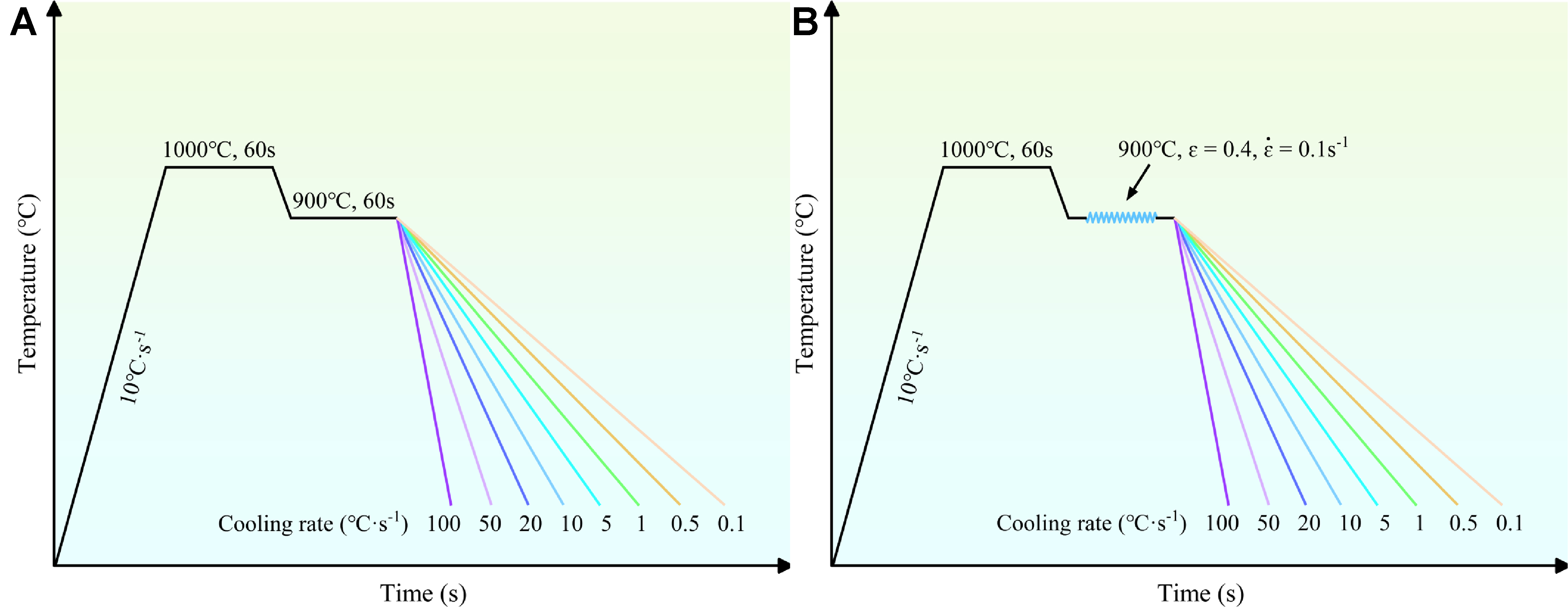
Figure 2. Flowchart of CCT experiments. (A) Static experiment; (B) Dynamic experiment. CCT: Continuous cooling transformation.
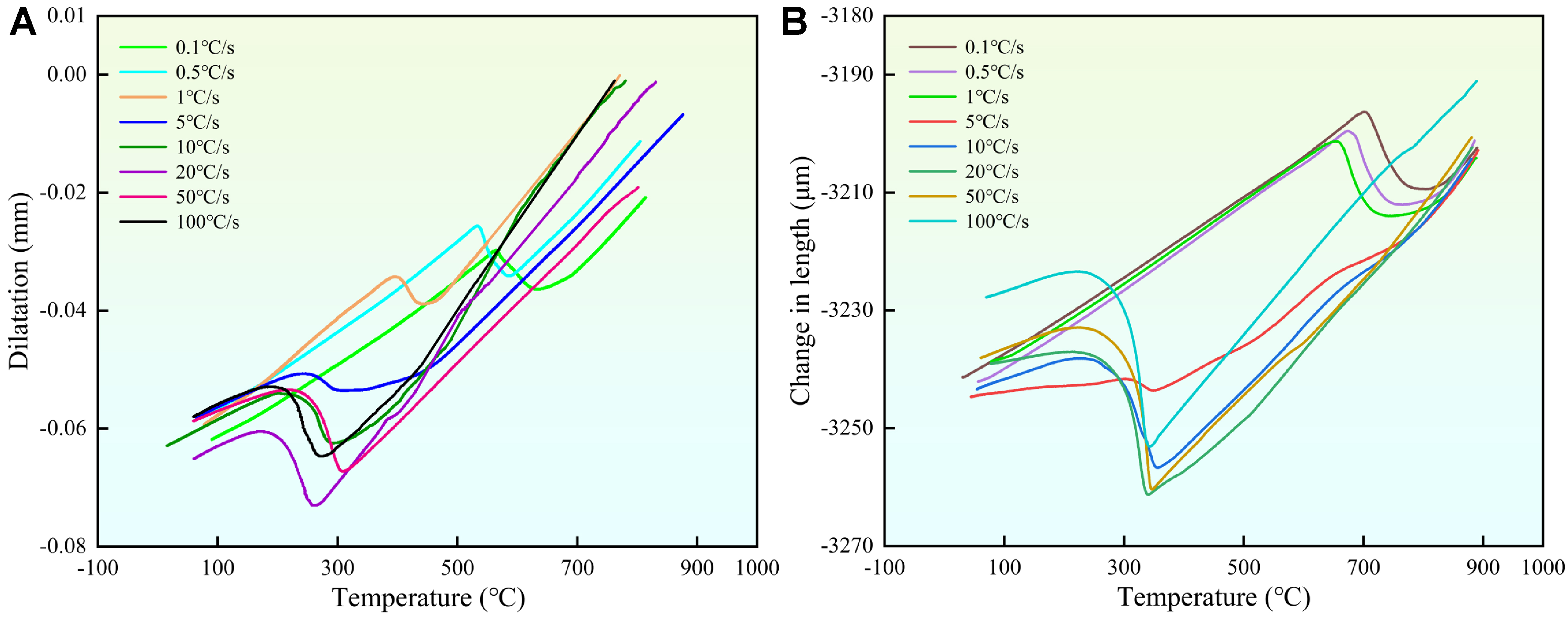
Figure 3. Dilatation curves of 30CrMnSi steel at different cooling rates. (A) Static experiment; (B) Dynamic experiment. Different colors and line styles represent different cooling rates as indicated in the legend.
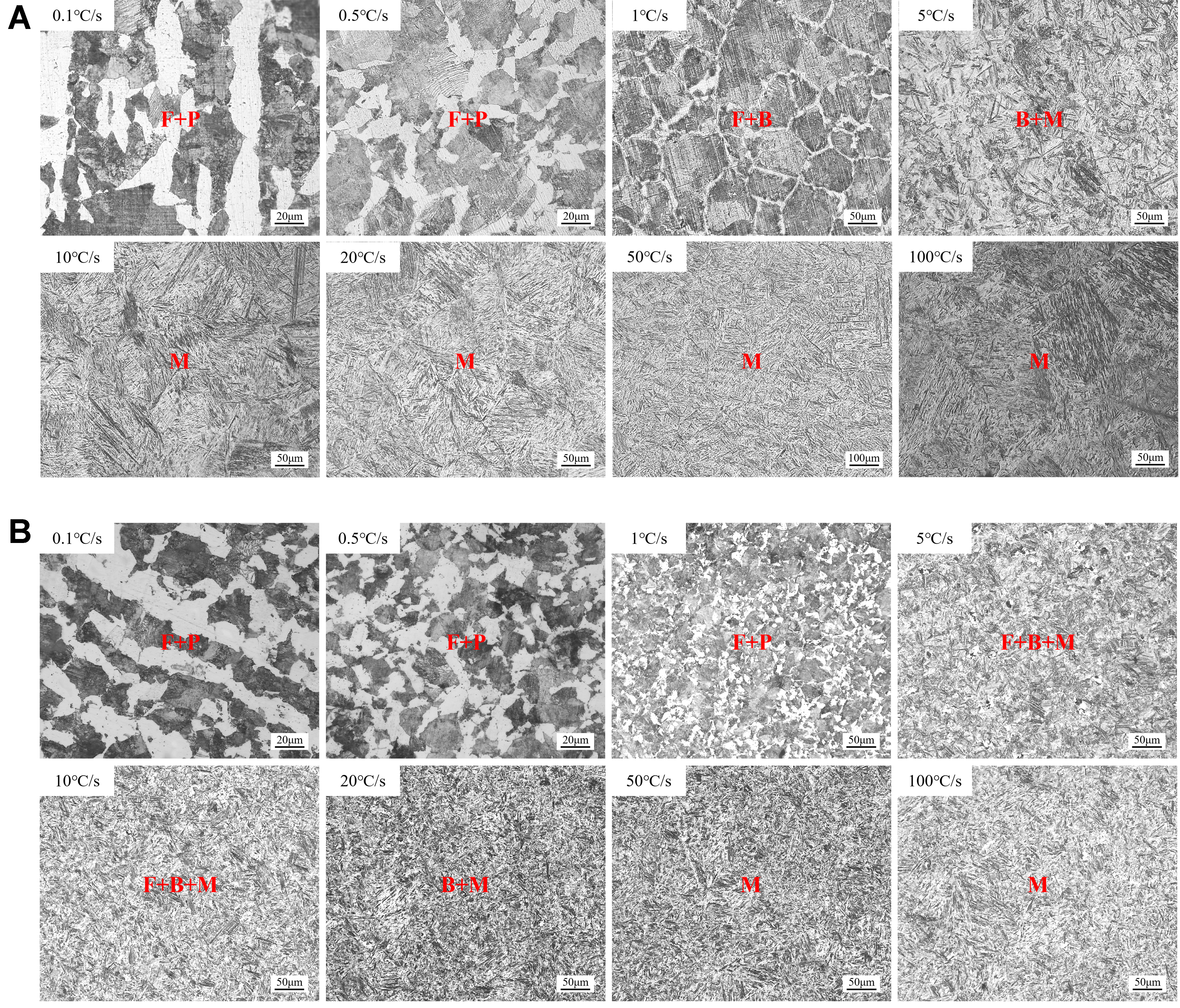
Figure 4. Microstructure of 30CrMnSi steel at different cooling rates. (A) Static specimen; (B) Dynamic specimen. F: Ferrite; P: pearlite; B: bainite; M: martensite.
Phase transformation points of static 30CrMnSi steel at different cooling rates
| Cooling rate (°C/s) | Fs | Ps | Bs | Ms | Ff | Pf | Bf | Mf |
| 0.1 | 701 ± 5 | 626 ± 7 | - | - | 566 ± 3 | 566 ± 3 | - | - |
| 0.5 | 697 ± 4 | 594 ± 2 | - | - | 529 ± 3 | 529 ± 3 | - | - |
| 1 | - | - | 483 ± 8 | - | - | - | 394 ± 4 | - |
| 5 | - | - | 471 ± 3 | 305 ± 2 | - | - | 305 ± 2 | 226 ± 3 |
| 10 | - | - | - | 314 ± 5 | - | - | - | 194 ± 4 |
| 20 | - | - | - | 276 ± 3 | - | - | - | 170 ± 4 |
| 50 | - | - | - | 313 ± 2 | - | - | - | 220 ± 6 |
| 100 | - | - | - | 290 ± 8 | - | - | - | 198 ± 6 |
Phase transformation points of dynamic 30CrMnSi steel at different cooling rates
| Cooling rate (°C/s) | Fs | Ps | Bs | Ms | Ff | Pf | Bf | Mf |
| 0.1 | 836 ± 4 | 780 ± 3 | - | - | 698 ± 2 | 698 ± 2 | - | - |
| 0.5 | 830 ± 4 | 752 ± 4 | - | - | 672 ± 1 | 672 ± 1 | - | - |
| 1 | 829 ± 5 | 740 ± 2 | - | - | 650 ± 4 | 650 ± 4 | - | - |
| 5 | 770 ± 2 | - | 541 ± 6 | 345 ± 4 | 644 ± 2 | - | 440 ± 5 | 290 ± 6 |
| 10 | 761 ± 6 | - | 533 ± 6 | 352 ± 3 | 645 ± 7 | - | 420 ± 4 | 228 ± 5 |
| 20 | - | - | 529 ± 5 | 346 ± 4 | - | - | 407 ± 6 | 220 ± 5 |
| 50 | - | - | - | 347 ± 2 | - | - | - | 220 ± 4 |
| 100 | - | - | - | 344 ± 2 | - | - | - | 219 ± 4 |
RESULTS AND DISCUSSION
Evaluation of ML model performance
The prediction performance of each ML model on the heldout test subset was comprehensively evaluated using three widely accepted statistical metrics: the R2, MAE, and RMSE. The R2 value quantifies how well the predicted values explain the observed variance, with a value closer to 1 indicating stronger explanatory power. MAE measures the average magnitude of the errors between predicted and actual values, providing an intuitive sense of prediction accuracy. RMSE penalizes larger errors more strongly. By employing these complementary metrics, the evaluation accounts for both the overall fit and the magnitude of prediction errors, thus providing a robust and logical assessment of model performance.
For the RF model, Figure 5 compares the predicted vs. measured values for the 8 phase transformation temperatures. All data points indicate that the model has extremely high predictive accuracy. As shown by the quantitative metrics in Supplementary Table 4, except for the Ps model (R2 = 0.977, MAE = 3.5 °C), the remaining seven transformation targets achieve R2 values at or above 0.99, with MAEs controlled around
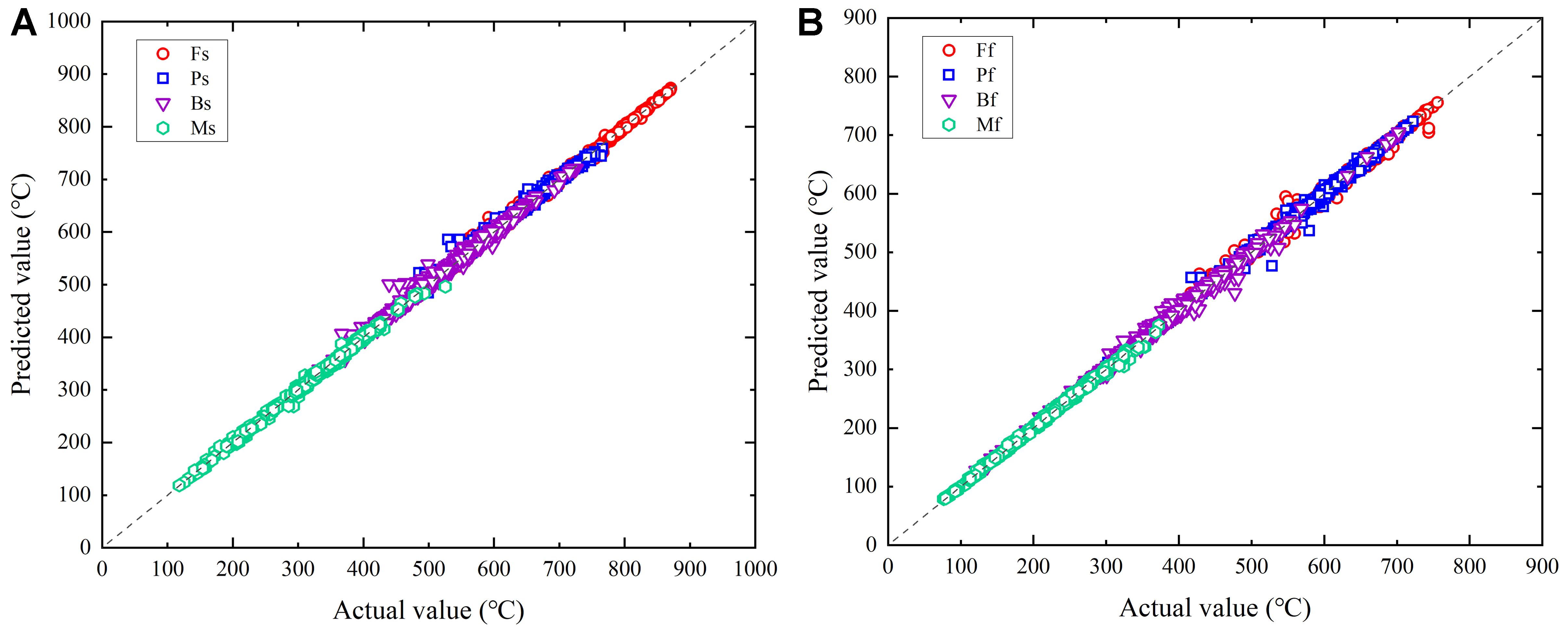
Figure 5. Comparison of RF model predictions with measured values. (A) Phase transformation start temperature; (B) Phase transformation finish temperature. RF: Random forest; Fs: ferrite transformation start temperature; Ps: pearlite transformation start temperature; Bs: bainite transformation start temperature; Ms: martensite transformation start temperature; Ff: ferrite transformation finish temperature; Pf: pearlite transformation finish temperature; Bf: bainite transformation finish temperature; Mf: martensite transformation finish temperature.
For the K-NN model, the scatter plot in Figure 6 shows that most predicted values for the target variables align closely with the actual values. This visual pattern suggests that the K-NN model generally captures the underlying relationships in the data. However, a closer examination of the quantitative results in Supplementary Table 5 reveals that the accuracy for Pf is affected by a relatively high RMSE of 14.5 °C. This elevated error may be attributed to the sensitivity of the K-NN algorithm to local outliers, where predictions can be significantly influenced by nearby anomalous data points. Despite this limitation, the model achieves a reasonable MAE of 3.5 °C for Pf, indicating that its typical prediction errors remain within an acceptable range. In addition, the K-NN model outperforms the RF model in predicting Ps, achieving a higher R2 value of 0.980. This superior R2 demonstrates that K-NN is particularly effective at capturing local patterns and features in the dataset.
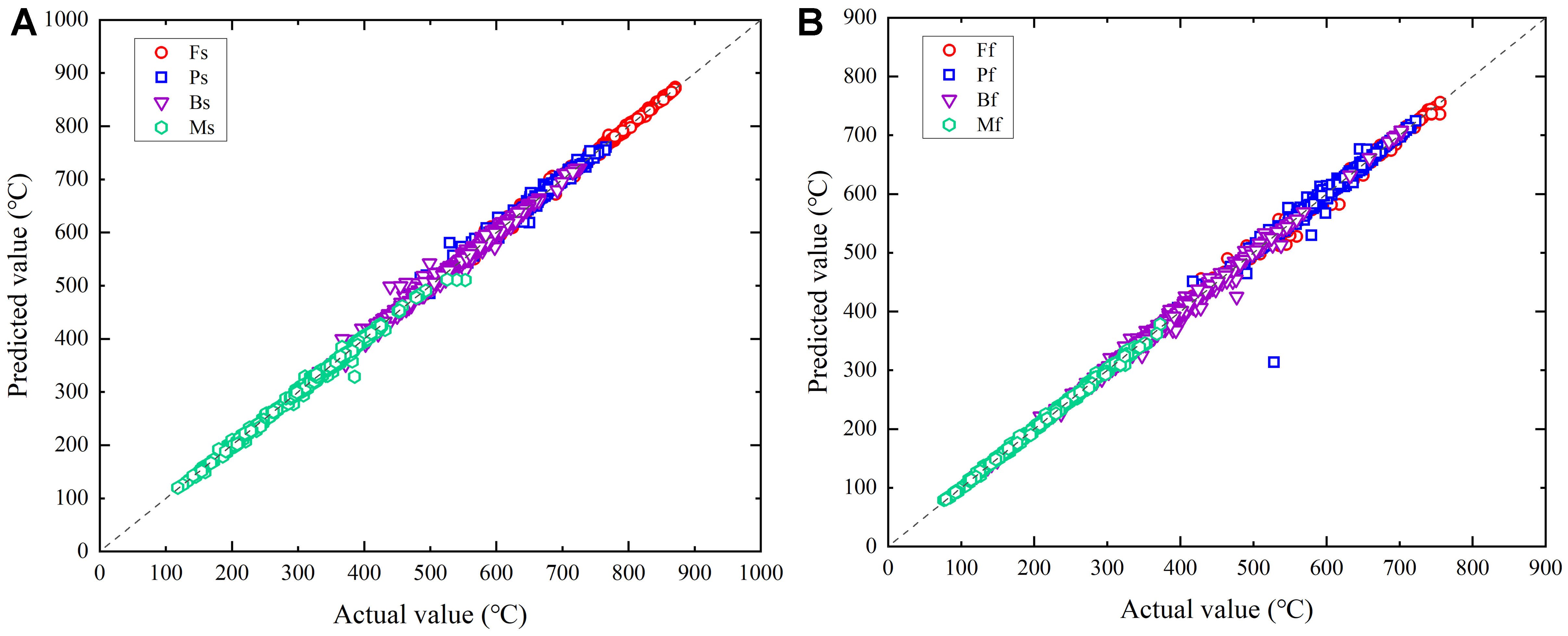
Figure 6. Comparison of K-NN model predictions with measured values. (A) Phase transformation start temperature; (B) Phase transformation finish temperature. K-NN: K-nearest neighbor; Fs: ferrite transformation start temperature; Ps: pearlite transformation start temperature; Bs: bainite transformation start temperature; Ms: martensite transformation start temperature; Ff: ferrite transformation finish temperature; Pf: pearlite transformation finish temperature; Bf: bainite transformation finish temperature; Mf: martensite transformation finish temperature.
A comprehensive evaluation was conducted to compare the performance of the two models across multiple aspects. The bar and line charts in Figure 7A-C visually compare important evaluation metrics for each model. This approach provides clear insight into where each model excels or struggles, highlighting differences in prediction quality for various targets. In addition, 10-fold cross-validation was performed separately for each phase transformation temperature, and the mean R2 values from cross-validation are summarized in Figure 7C. The RF model consistently achieved mean R2 [cross-validation (CV)] values above 0.980 for all target temperatures, indicating high predictive accuracy and robust performance. In contrast, the mean R2 (CV) values for the K-NN model fluctuated significantly and were generally lower than those of the RF model, demonstrating less consistent performance and greater sensitivity to specific data partitions. This inconsistency means that although K-NN can achieve high accuracy for some individual phase transformation temperatures, it does not deliver stable results across all targets. Overall, the RF model demonstrates superior stability in predicting the eight phase transformation temperatures.
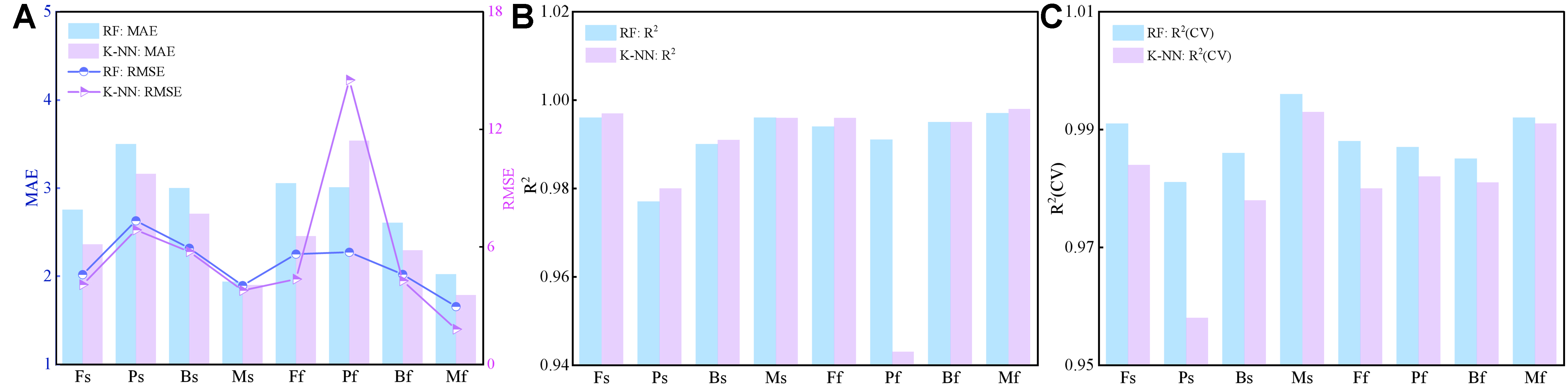
Figure 7. Comparison of evaluation metrics between the RF and K-NN models. (A) MAE & RMSE; (B) R2; (C) R2 from 10-fold cross-validation. RF: Random forest; K-NN: k-nearest neighbor; MAE: mean absolute error; RMSE: root mean square error; R2: coefficient of determination; CV: cross-validation; Fs: ferrite transformation start temperature; Ps: pearlite transformation start temperature; Bs: bainite transformation start temperature; Ms: martensite transformation start temperature; Ff: ferrite transformation finish temperature; Pf: pearlite transformation finish temperature; Bf: bainite transformation finish temperature; Mf: martensite transformation finish temperature.
To further examine the independence of the test set, we conducted exploratory validation using stricter grouping protocols: GroupKFold with each complete CCT curve treated as one group, leave-one-steel-grade-out validation, and leave-one-source-publication-out validation. These stricter partitioning tests show degraded prediction performance, which qualitatively indicates limited extrapolation ability to unseen steel grades. Given the limited diversity of the current database, the quantitative results from these strict-group validations are not sufficiently robust for formal quantitative analysis in this work. Therefore, the high R2 and low MAE values reported above should be interpreted as model performance under the original 7:3 random partitioning, focusing on predictions within the collected conditions, rather than evidence of reliable generalization to entirely new steel grades. Expanding the CCT database and carrying out comprehensive quantitative strict-group validation will be pursued as future work.
Global feature importance analysis
Unlike traditional PM models, ML models present interpretability challenges because internal prediction processes cannot be directly described by established mathematical or physical laws. To overcome this limitation and clarify the process by which ML models make predictions and how input features contribute, this study adopted the SHAP method. This method yields quantitative measures of global feature importance for all input variables. Figure 8A-H provides a comprehensive visualization of the average impact of each feature on predictions for the start and finish temperatures of eight distinct phase transformation temperatures, as well as the influence direction of each feature. This interpretability analysis allows for a deeper understanding of model operation and the physical meaning of important input variables. To facilitate detailed inspection of each transformation temperature, individual high-resolution SHAP summary plots are provided in Supplementary Figures 2-9.
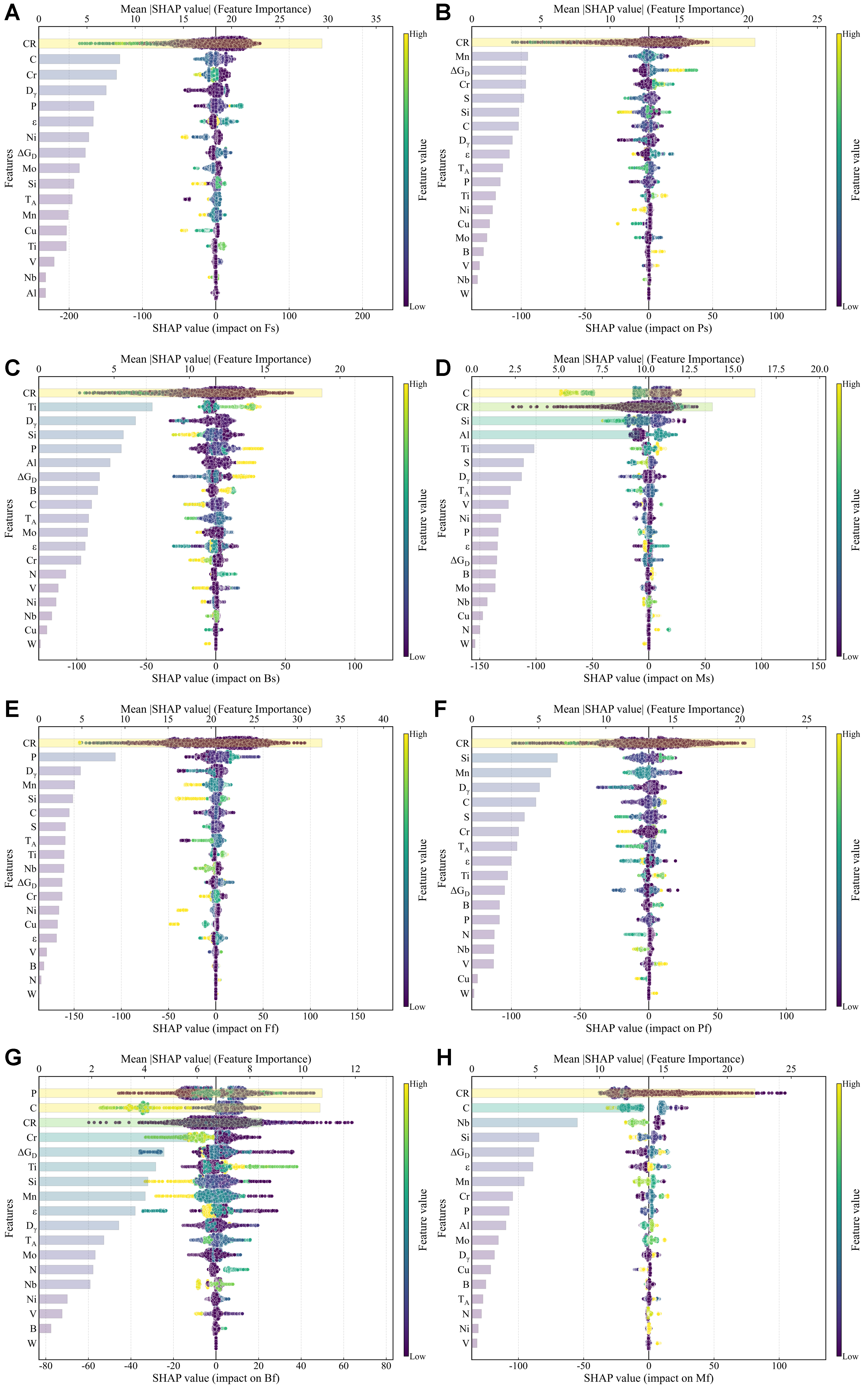
Figure 8. Analysis of the influence of input features on phase transformation temperatures and feature importance based on SHAP. (A) Fs; (B) Ps; (C) Bs; (D) Ms; (E) Ff; (F) Pf; (G) Bf; (H) Mf. SHAP: SHapley Additive exPlanations. ΔGD: dislocation energy; Dγ: austenite grain size; TA: austenitizing temperature.
Analysis identifies CR as the most influential variable for predicting phase transformation temperatures, including Fs, Ps, Bs, Ff, Pf, and Mf. For Ms, carbon content becomes the primary determining factor. A negative SHAP value for carbon content indicates that higher carbon content produces a lower Ms, which is consistent with established PM principles reported in the literature[19,20,39]. Additional elements, such as Cr, Ni, and Si, also exert effects on specific phase transformation temperatures that agree with previously published findings. These consistent observations further support the reliability and scientific validity of the model interpretability framework.
A key result involves the significant contribution of the two supplementary features, ΔGD and Dγ, which originate from PM model calculations and are incorporated into the input dataset. For example, ΔGD ranks third in importance for the Ps model and fifth for both the Bf and Mf models, while Dγ achieves third place in Bs and Ff models and fourth in the Fs and Pf models based on SHAP analysis. This evidence strongly supports the value of integrating physically informed features into a ML framework. Incorporating variables that represent metallurgical deformation mechanisms enables the hybrid approach to capture essential influences on phase transformation behavior, effectively bridging the gap between data-driven modeling and physically based understanding.
To further quantify the contribution of the PM-derived features, we compared model performance with and without ΔGD and Dγ as inputs. As shown in Supplementary Figures 10 and 11, adding these two features consistently improves R2 and reduces MAE for most transformation temperatures across both RF and K-NN models. This confirms that the PM-guided feature engineering enhances predictive accuracy beyond the baseline composition and thermal parameters.
Analysis of how deformation affects phase transformation temperatures
To further investigate deformation effects, the dependence plot generated by SHAP analysis revealed how the supplementary input feature, dislocation energy ΔGD, influences the phase transformation temperature [Figure 9A-H]. When ΔGD increases, SHAP values for Fs, Ps, Bs, Ff, and Mf also increase, which is qualitatively consistent with the underlying physical mechanism: deformation accelerates phase transformation kinetics. For diffusion-type phase transformations such as ferrite and pearlite, high-density dislocations and subgrains introduced via deformation supply additional nucleation sites. A greater amount of deformation storage energy strengthens the driving force for the phase transformation, increases the diffusion efficiency of elements, and results in higher transformation temperatures. bainite phase transformation mechanism shows considerable complexity; multiple authors report inconsistent results due to varying deformation and transformation conditions[40]. Nevertheless, a broad consensus exists that deformation of austenite leads to a faster bainite transformation rate, a higher initial transformation temperature, and a wider bainite transformation region in the CCT diagram[41-43]. These findings align with model output, which shows an increase in Bs as ΔGD rises. For Ms, deformation exerts minimal influence, reflecting the model ability to recognize that non-diffusive phase transformations respond more to chemical composition than to strain.
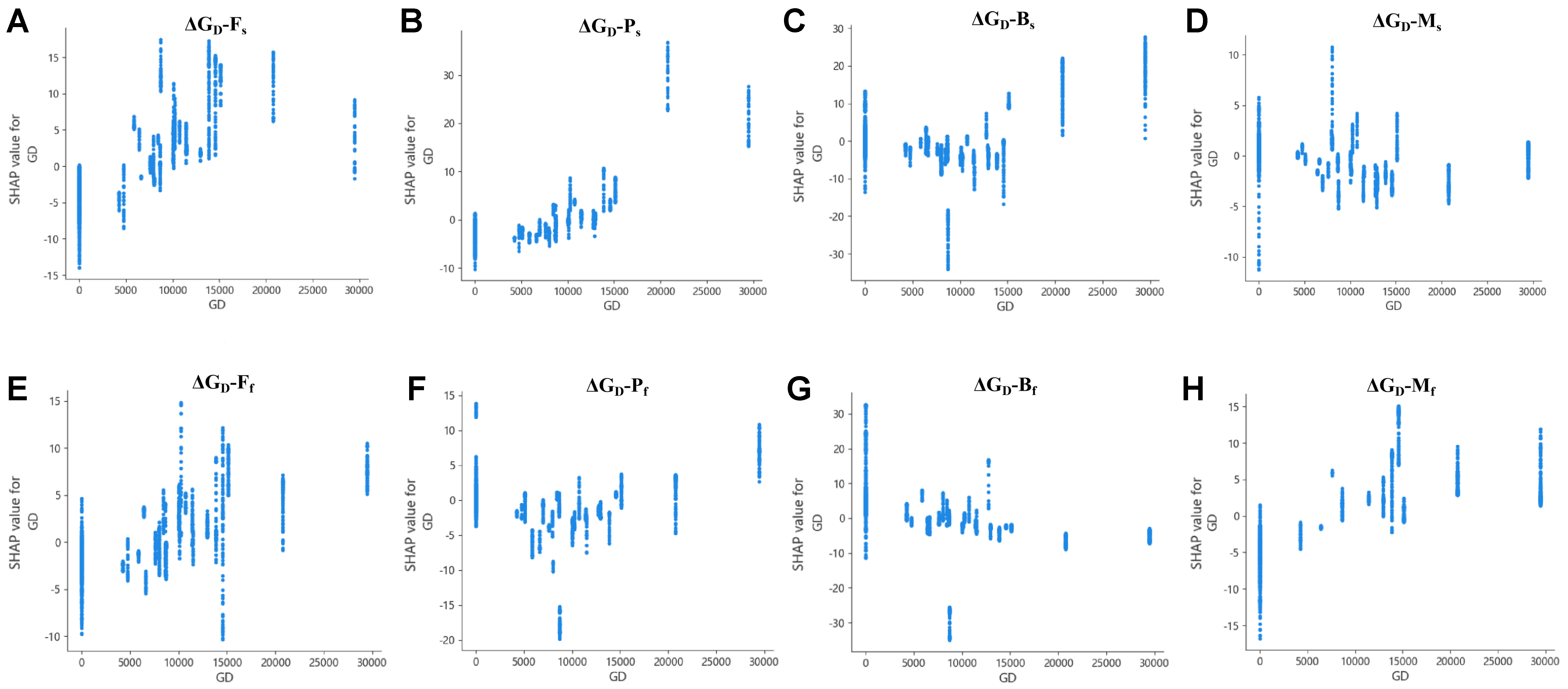
Figure 9. SHAP analysis of the effect of ΔGD on phase transformation temperature prediction. (A) Fs; (B) Ps; (C) Bs; (D) Ms; (E) Ff; (F) Pf; (G) Bf; (H) Mf. SHAP: SHapley Additive exPlanations; ΔGD: dislocation energy; Fs: ferrite transformation start temperature; Ps: pearlite transformation start temperature; Bs: bainite transformation start temperature; Ms: martensite transformation start temperature; Ff: ferrite transformation finish temperature; Pf: pearlite transformation finish temperature; Bf: bainite transformation finish temperature; Mf: martensite transformation finish temperature.
Validation results based on thermal expansion tests
Experimentally measured static and dynamic CCT curves for 30CrMnSi steel served as benchmarks for evaluating prediction accuracy of both RF and K-NN models, as displayed in Figure 10A and B. These figures also present a direct comparison with results obtained using JMatPro commercial software, providing a comprehensive view of predictive capabilities across all approaches.
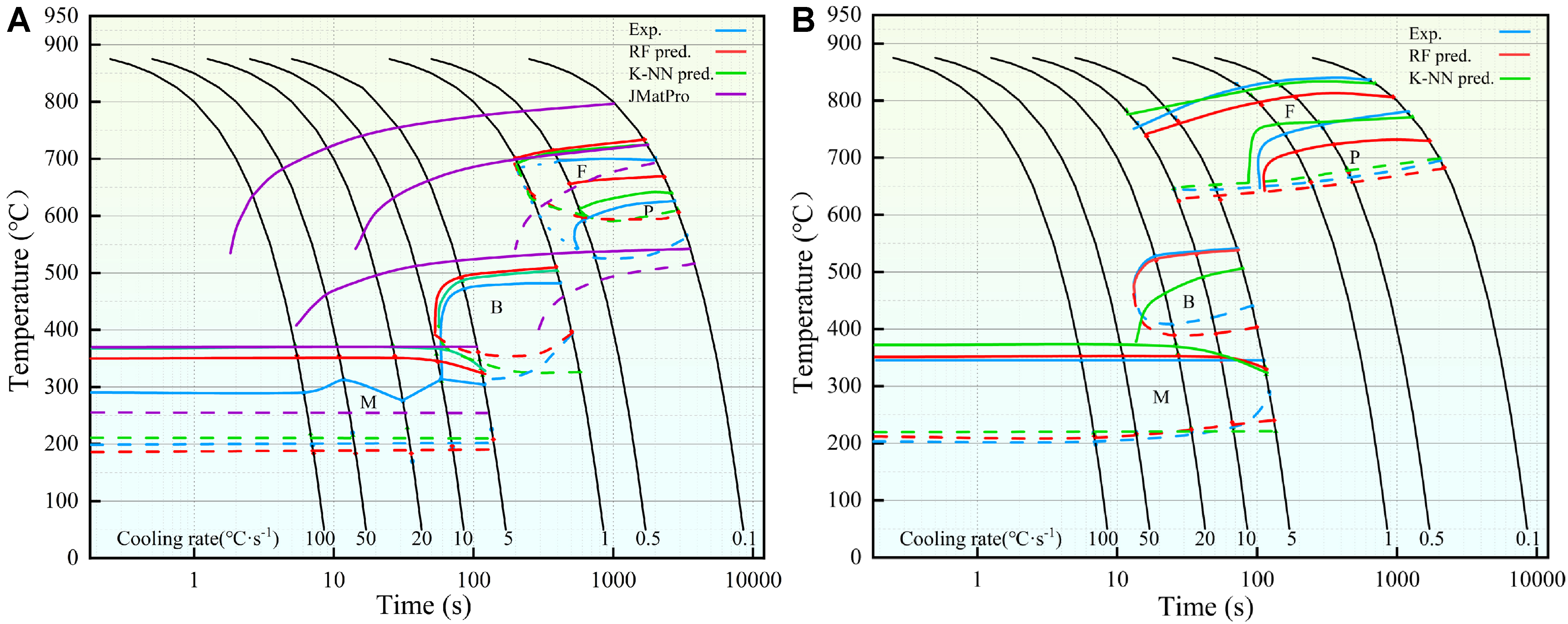
Figure 10. Comparison of experimental CCT curves with model-predicted CCT curves. (A) Static CCT; (B) Dynamic CCT. CCT: Continuous cooling transformation; Exp.: experimental value; RF pred.: random forest predicted value; K-NN pred.: k-nearest neighbor predicted value.
Examination of the static CCT curve in Figure 10A demonstrates that both ML models produced reliable and accurate results. For Fs and Bs, predicted values showed close alignment with experimental measurements, and error magnitude decreased as CR increased. MAE for these transformations remained below 25.0 °C, indicating robust model performance. The K-NN model achieves an MAE of 15.0 °C for Ps, while the RF model gives 54.5 °C, representing a reduction of about 39.5 °C with K-NN. This substantial difference may result from overfitting in the RF approach. In contrast, the RF model gave better predictions for Ms, with an average absolute error of 34.0 °C, a 13.0 °C improvement over the K-NN model. This performance likely arises from the ensemble learning framework within the RF model, which enables effective management of complex interactions among alloying elements, an important requirement for accurate Ms prediction. The K-NN model, which relies on distance-based calculations, cannot fully capture such multidimensional relationships. For Pf at low cooling rates, both models showed notable prediction deviations, likely due to a small number of relevant training samples and variability in experimental datasets. For Mf, both models maintained strong agreement with experimental values. In comparison, JMatPro commercial software produced much larger errors for ferrite and pearlite transformation temperatures (~100.0 °C), as well as substantial inaccuracies for Bs and Ms. JMatPro also failed to identify critical cooling rates for phase transformations.
Evaluation of dynamic CCT curves in Figure 10B reveals even stronger advantages for the ML approach. The K-NN model provided accurate predictions for increased transformation temperatures of ferrite and pearlite after deformation, achieving an average absolute error of 10.0 °C for ferrite. For pearlite, prediction accuracy decreased slightly as CR increased. The RF model demonstrated slightly lower accuracy than the K-NN for these two diffusion-controlled transformations. For Bs and Ms, the RF model delivered outstanding results, with average absolute error consistently at 5.0 °C or less, while K-NN produced less accurate predictions for these transformations. For transformation finish temperatures (Ff, Pf, and Mf), both models gave reliable results. Notably, both models captured major physical phenomena associated with deformation, including increased start temperatures for phase transformations, leftward shifting of CCT curves (corresponding to shorter transformation times at a given temperature, i.e., accelerated transformation kinetics), and expansion of transformation regions for ferrite and pearlite. The ML model developed for this study, enhanced with supplementary features based on PM, effectively learned and reproduced the complex effects of thermal deformation on phase transformation behavior. This methodological approach resulted in predictive performance far superior to conventional commercial software.
Incorporating a PM parameter in this study enabled the model to replicate several essential features observed in dynamic CCT curves, including an increased onset temperature and a leftward shift of diffusion-type phase transformations. These phenomena result from enhanced energy storage due to deformation, a factor widely considered crucial in phase transformation kinetics. Although the model captured these core effects, closer examination uncovers limitations that require further discussion. Validation performed by Hedström et al. showed that the largest deviations in Bs prediction occurred for specimens subjected to deformation before cooling[44]. That analysis highlighted a persistent challenge in modeling, i.e., difficulty in representing the full complexity of thermal deformation history. Most models, including the approach used here, apply simplified PM parameters that aggregate deformation effects into a single or limited set of variables. Such a method cannot fully represent the broad spectrum of microstructural changes caused by real thermal deformation. For instance, changes in grain boundary character, spatial distribution of dislocations, and formation of sub-grains or deformation twins, all phenomena that influence phase transformation behavior, are not captured by a single PM parameter.
Consequently, while trends for Fs, Ps, Bs, and related transformations are reasonably well predicted, notable deviations remain under dynamic conditions, especially for transformation finish temperatures such as Bf. This finding indicates that future models should incorporate more granular microstructural descriptors, potentially using data from advanced characterization techniques or multiscale simulations. Techniques including electron backscatter diffraction (EBSD), transmission electron microscopy (TEM), or three-dimensional atom probe tomography (APT) can provide information on grain orientation, dislocation density, and solute segregation, leading to a more physically accurate representation. Enhanced models would then be better suited to address the subtleties of medium-temperature transformations such as bainite, where multiple mechanisms, diffusional and displacive, interact in complex ways.
The RF model, despite improved performance over other approaches, produced an average absolute error of 34 °C when predicting static Ms. This level of error, although lower than some values reported in the literature, still poses concerns for practical applications. Hedström et al. documented errors in Ms prediction exceeding 130 °C for certain high-carbon, high-chromium steels, attributing much of this discrepancy to reliance on nominal composition as model input[44]. Using nominal composition overlooks the actual chemical state of austenite, especially in cases where carbide precipitation or incomplete dissolution changes the distribution of carbon and alloying elements. Ms temperature is highly sensitive to the precise chemical composition of austenite, with minor deviations in C or substitutional element content causing substantial changes in the transformation temperature. In 30CrMnSi steel, this issue is further intensified by the presence of carbide-forming elements such as Cr. Austenitizing treatments might not fully dissolve carbides or cause segregation, resulting in a mismatch between the nominal and effective matrix composition. This composition gap explains why even advanced ML models that rely solely on nominal values struggle to achieve higher accuracy for Ms prediction.
Deeper integration of thermodynamic modeling and experimental microanalysis into data-driven frameworks could help address this limitation. For example, future models may use effective austenite composition, estimated by thermodynamic calculations or measured using techniques such as electron probe microanalysis (EPMA), to replace or supplement nominal composition as an input feature. In addition, including Ms values calculated from empirical formulas as an auxiliary feature would allow a ML model to learn systematic residuals and thus combine empirical knowledge with data-driven insight. Such hybrid approaches would substantially increase the fidelity and reliability of phase transformation predictions, especially for complex alloy systems and key transformation points such as Ms.
Moreover, it should be emphasized that the present study’s training and test data were derived from the same collection of literature CCT curves, with each data point intrinsically linked to its parent curve, steel grade, and source publication. While the random 7:3 split adopted in this work enables evaluation of fitting and prediction within the known data scope, it cannot rule out information overlap between the training and test sets. Stricter validations confirmed that the model’s extrapolation capability to entirely new steel grades remains limited. Future efforts will focus on enlarging the database with more diverse and independent CCT curves, incorporating physical constraints, and exploring nested validation to enhance model generalizability.
CONCLUSIONS
(1) A ML prediction framework was developed to address the limitations of conventional modeling. PM information was incorporated through supplementary features, specifically dislocation energy and austenite grain size derived from established metallurgical principles. These features enabled RF and K-NN models to represent the influence of thermal deformation mechanisms with greater accuracy. Evaluated using the internal random-split test set for eight phase-transformation temperatures, the models exhibit generally high predictive performance, with R2 mostly at or above 0.99 and MAE mostly below 3.0 °C. Exceptions include Ps for the RF model (R2 = 0.977, MAE = 3.5 °C), Ps for the K-NN model (R2 = 0.980, MAE = 3.2 °C), and Pf for the K-NN model (R2 = 0.943, MAE = 3.5 °C). Overall, the developed models still achieve evident improvements over empirical and conventional data-driven methods.
(2) SHAP interpretability assessment identified cooling rate and carbon content as the most influential factors in phase transformation predictions. Addition of physically derived features Dγ and ΔGD further enhanced prediction accuracy. Dependence analysis showed that the model outputs are qualitatively consistent with key metallurgical principles, such as the effect of increased ΔGD in raising transformation temperatures for ferrite, pearlite, and bainite.
(3) Experimental validation on static and dynamic CCT curves of 30CrMnSi steel shows that the proposed modeling framework can provide predictions consistent with experimental data, including the leftward shift (transformation to shorter times) of CCT curves induced by deformation. For this tested condition, both RF and K-NN models outperform mainstream commercial tools.
DECLARATIONS
Authors’ contributions
Conceptualization: Yang, J.; Zhao, W.; Hou, Z.; Huang, X.
Methodology: Yang, J.; Zhao, W.; Lu, B.; Hou, Z.
Investigation: Yang, J.; Zhao, W.; Lu, B.
Funding acquisition: Hou, Z.; Huang, X.
Project administration: Hou, Z.
Supervision: Hou, Z.; Mu, W.; Huang, X.
Writing - original draft: Yang, J.; Zhao, W.; Lu, B.; Hou, Z.
Writing - review and editing: Yang, J.; Zhao, W.; Lu, B.; Mu, W.; Huang, X.; Hou, Z.
Availability of data and materials
The original contributions presented in this study are included in the article/Supplementary Materials. Further inquiries can be directed to the corresponding author.
AI and AI-assisted tools statement
Not applicable.
Financial support and sponsorship
This work was supported by the National Key Research and Development Program of
China (2024YFB3713703), National Natural Science Foundation of China (52574428), the Foundation for Innovative Research Groups of the National Natural Science Foundation of China (T2421001), and the Fundamental Research Funds for the Central Universities of China (2024IAIS-ZD004, 2025CDJZKPT-03).
Conflicts of interest
All authors declared that there are no conflicts of interest.
Ethical approval and consent to participate
Not applicable.
Consent for publication
Not applicable.
Copyright
© The Author(s) 2026.
Supplementary Materials
REFERENCES
1. Geng, X.; Wang, F.; Wu, H.; et al. Data‐driven and artificial intelligence accelerated steel material research and intelligent manufacturing technology. Mater. Genome. Eng. Adv. 2023, 1, e10.
2. Fang, W.; Huang, J.; Peng, T.; Long, Y.; Yin, F. Machine learning-based performance predictions for steels considering manufacturing process parameters: a review. J. Iron. Steel. Res. Int. 2024, 31, 1555-81.
3. Yu, X.; Tan, C. China’s pathway to carbon neutrality for the iron and steel industry. Glob. Environ. Change. 2022, 76, 102574.
4. Wang, H.; Qiu, J.; Ping, X.; et al. Roadmap, current situation, and prospects of low-carbon development technologies in Chinese steel industry. J. Iron. Steel. Res. Int. 2024, 31, 2879-92.
5. Kang, Z.; Liao, Q.; Zhang, Z.; Zhang, Y. Carbon neutrality orientates the reform of the steel industry. Nat. Mater. 2022, 21, 1094-8.
6. Gutiérrez Castañeda, E.; Ruiz Cigarrillo, D.; Torres Castillo, A.; et al. Intercritical continuous cooling transformation diagram for the manufacture of low-alloyed low-carbon multiphase steels. Mater. Lett. 2023, 331, 133528.
7. Geng, X.; Wang, H.; Xue, W.; et al. Modeling of CCT diagrams for tool steels using different machine learning techniques. Comput. Mater. Sci. 2020, 171, 109235.
8. Cao, Y.; Cao, G.; Cui, C.; Li, X.; Wu, S.; Liu, Z. Modeling continuous cooling transformations for HSLA steels with physical metallurgy guided hereditary machine learning. Metall. Mater. Trans. A. 2023, 54, 4891-904.
9. Xu, P.; Ji, X.; Li, M.; Lu, W. Small data machine learning in materials science. npj. Comput. Mater. 2023, 9, 1000.
10. Gao, Z.; Wu, S.; Zhou, X.; et al. Physical-informed machine learning of phase transformation and application to cooling path optimization. J. Iron. Steel. Res. Int. 2026, 33, 1822.
11. Huang, X.; Zhang, B.; Tian, Q.; et al. Machine learning study on time–temperature–transformation diagram of carbon and low-alloy steel. J. Iron. Steel. Res. Int. 2023, 30, 1032-41.
12. Cao, G.; He, Y.; Wang, H.; et al. Machine learning assisted adaptable rolling for high strength steel. J. Iron. Steel. Res. Int. 2026, 33, 1645.
13. Geng, X.; Wang, H.; Ullah, A.; et al. Prediction of continuous cooling transformation diagrams for Ni-Cr-Mo welding steels via machine learning approaches. JOM 2020, 72, 3926-34.
14. Minamoto, S.; Tsukamoto, S.; Kasuya, T.; Watanabe, M.; Demura, M. Prediction of continuous cooling transformation diagram for weld heat affected zone by machine learning. Sci. Technol. Adv. Mater. Methods. 2022, 2, 402-15.
15. Geng, X.; Mao, X.; Wu, H.; et al. A hybrid machine learning model for predicting continuous cooling transformation diagrams in welding heat-affected zone of low alloy steels. J. Mater. Sci. Technol. 2022, 107, 207-15.
16. Zhang, B.; Wang, B.; Xue, W.; Ullah, A.; Zhang, T.; Wang, H. Development of a machine learning model for prediction of continuous cooling transformation diagrams in welding heat-affected zone. J. Mater. Sci. 2023, 58, 4795-808.
17. Rahaman, M.; Mu, W.; Odqvist, J.; Hedström, P. Machine learning to predict the martensite start temperature in steels. Metall. Mater. Trans. A. 2019, 50, 2081-91.
18. Jeon, J.; Sung, Y.; Seo, N.; Jung, J.; Son, S. B.; Lee, S. Machine learning model and prediction mechanisms of bainite start temperature of low alloy steels. Mater. Trans. 2023, 64, 2214-8.
19. Jeon, J.; Seo, N.; Jung, J.; Son, S. B.; Lee, S. Analysis of prediction mechanisms and feature importance of martensite start temperature of alloy steel via explainable artificial intelligence. Mater. Trans. 2023, 64, 2196-201.
20. Zhang, Y.; Cheng, L.; Pan, A.; Hu, C.; Wu, K. Phase transformation temperature prediction in steels via machine learning. Materials 2024, 17, 1117.
21. Dobrzański, L. A.; Trzaska, J. Application of neural networks for the prediction of continuous cooling transformation diagrams. Comput. Mater. Sci. 2004, 30, 251-9.
22. Trzaska, J.; Dobrzański, L. Modelling of CCT diagrams for engineering and constructional steels. J. Mater. Process. Technol. 2007, 192-3, 504-10.
23. Trzaska, J. A new neural networks model for calculating the continuous cooling transformation diagrams. Arch. Metall. Mater. 2018, 63, 2009-15.
24. Chakraborty, S.; Chattopadhyay, P. P.; Ghosh, S. K.; Datta, S. Incorporation of prior knowledge in neural network model for continuous cooling of steel using genetic algorithm. Appl. Soft. Comput. 2017, 58, 297-306.
25. Chakraborty, S.; Das, P.; Kaveti, N. K.; Chattopadhyay, P. P.; Datta, S. MCDM towards knowledge incorporation in ANN models for phase transformation in continuous cooling of steel. Multidiscip. Model. Mater. Struct. 2019, 15, 170-86.
26. Ganguly, S.; Manna, S. Prediction of continuous cooling transformation diagrams in steels using light gradient boosting and rule-based optimization. Mater. Manuf. Process. 2023, 38, 2018-33.
27. Liang, W.; Li, J.; Li, J.; Xiong, X.; Chai, J. Hot deformation characteristics and microstructure evolution of industrial grade AISI M35 high-speed steel produced by ESR. J. Iron. Steel. Res. Int. 2025, 32, 2370-88.
28. Zhang, M.; Wang, C.; Ma, D.; et al. Influence of hot deformation on dynamic recrystallization behavior of a novel austenitic stainless steel. J. Iron. Steel. Res. Int. 2025, 32, 4335-49.
29. Li, X.; Zheng, M.; Pan, H.; Mao, C.; Ding, W. An integrated design of novel RAFM steels with targeted microstructures and tensile properties using machine learning and CALPHAD. J. Mater. Inf. 2024, 4, 27.
30. Song, L.; Wang, C.; Li, Y.; Wei, X. Predicting stacking fault energy in austenitic stainless steels via physical metallurgy-based machine learning approaches. J. Mater. Inf. 2025, 5, 2.
31. Hart-Rawung, T.; Buhl, J.; Bambach, M. A fast approach for optimization of hot stamping based on machine learning of phase transformation kinetics. Procedia. Manuf. 2020, 47, 707-12.
32. Hatta, N.; Kokado, J.; Kikuchi, S.; Takuda, H. Modelling on flow stress of plain carbon steel at elevated temperatures. Steel. Res. 1985, 56, 575-82.
33. Medina, S.; Hernandez, C. General expression of the Zener-Hollomon parameter as a function of the chemical composition of low alloy and microalloyed steels. Acta. Mater. 1996, 44, 137-48.
34. Suwanpinij, P.; Rudnizki, J.; Prahl, U.; Bleck, W. Investigation of the effect of deformation on γ‐α phase transformation kinetics in hot-rolled dual phase steel by phase field approach. Steel. Res. Int. 2009, 80, 616-22.
35. Wang, S.; Li, J.; Zeng, L.; Zuo, X.; Chen, N.; Rong, Y. Machine learning for prediction of retained austenite fraction and optimization of processing in quenched and partitioned steels. J. Iron. Steel. Res. Int. 2024, 31, 2002-13.
36. Bassi, A.; Bodas, S. T.; Hasan, S. S.; Sidhu, G.; Srinivasan, S. Predictive modeling of hardness values and phase fraction percentages in micro-alloyed steel during heat treatment using AI. Metals 2024, 14, 49.
37. Li, F.; He, A.; Song, Y.; et al. Deep learning for predictive mechanical properties of hot-rolled strip in complex manufacturing systems. Int. J. Miner. Metall. Mater. 2023, 30, 1093-103.
38. Bräutigam–Matus, K.; Altamirano, G.; Salinas, A.; Flores, A.; Goodwin, F. Experimental determination of continuous cooling transformation (CCT) diagrams for dual-phase steels from the intercritical temperature range. Metals 2018, 8, 674.
39. Liu, C.; Su, H. Prediction of martensite start temperature of steel combined with expert experience and machine learning. Sci. Technol. Adv. Mater. 2024, 25, 2354655.
40. Xiao, F.; Liao, B.; Qiao, G.; Guan, S. Effect of hot deformation on phase transformation kinetics of 86CrMoV7 steel. Mater. Charact. 2006, 57, 306-13.
41. Nikravesh, M.; Naderi, M.; Akbari, G.; Bleck, W. Phase transformations in a simulated hot stamping process of the boron bearing steel. Mater. Design. 2015, 84, 18-24.
42. Kawulok, R.; Kawulok, P.; Schindler, I.; et al. Study of the effect of deformation on transformation diagrams of two low-alloy manganese-chromium steels. Arch. Metall. Mater. 2018, 63, 1735-41.
43. Zhang, R.; Boyd, J. Bainite transformation in deformed austenite. Metall. Mater. Trans. A. 2010, 41, 1448-59.
Cite This Article
 Open Access
How to Cite
Yang, J.; Zhao, W.; Lu, B.; Mu, W.; Huang, X.; Hou, Z. Integrating physical metallurgy principles and machine learning for predicting continuous cooling phase transformations in steel. J. Mater. Inf. 2026, 6, 48. https://dx.doi.org/10.20517/jmi.2026.54
Download Citation
If you have the appropriate software installed, you can download article citation data to the citation manager of your choice. Simply select your manager software from the list below and click on download.
Export Citation File
Type of Import
Tips on Downloading Citation
Citation Manager File Format
Type of Import
Direct Import: When the Direct Import option is selected (the default state), a dialogue box will give you the option to Save or Open the downloaded citation data. Choosing Open will either launch your citation manager or give you a choice of applications with which to use the metadata. The Save option saves the file locally for later use.
Indirect Import: When the Indirect Import option is selected, the metadata is displayed and may be copied and pasted as needed.
About This Article
Copyright

Data & Comments
Data
0











Comments
Comments must be written in English. Spam, offensive content, impersonation, and private information will not be permitted. If any comment is reported and identified as inappropriate content by OAE staff, the comment will be removed without notice. If you have any queries or need any help, please contact us at [email protected].