Simple formula learned via machine learning for creep rupture life prediction of high-temperature titanium alloys
Abstract
Creep behavior of high-temperature titanium alloys determines their service life and thereby prediction of creep rupture life is in demand due to the costly and time-consuming measurements. Machine learning (ML) has been employed to build surrogate models for creep rupture life; however, the commonly used algorithms are often black-box due to the pursuit of high accuracy. Here, we first show that multiple linear regression (MLR) can result in models or formulae with much higher accuracy than those based on typical black-box methods. Furthermore, by combining feature selection and symbolic regression, we obtain a simple and unified formula for accurately predicting the creep rupture life of high-temperature titanium alloys. The formula is learned using the short-term creep rupture life data and consists of merely three attributes, that is, the Molybdenum equivalent, the test stress and test temperature. It outperforms the MLR models and generalizes well to different testing data with varying long-term creep rupture life. The simple formula can be readily applied to new titanium alloys for predicting the creep rupture life and is easily accessible to experimentalists in the materials community.
Keywords
INTRODUCTION
High-temperature titanium alloys are frequently utilized in vital aerospace components because of their exceptional properties, such as high specific strength [1–4]. The durability of high-temperature structural components primarily relies on the creep behavior of alloys [5]. Plastic deformation associated with creep behavior under fixed temperature and stress can induce fracture incidents [6]. Given the costly and laborious experimental synthesis and measurement, much attention has been devoted to developing prediction methods [7,8]. Typical examples include empirical and theoretical models, as well as those based on machine learning (ML), which can expedite the assessment of creep properties [9–15].
The empirical and theoretical models can be roughly classified into two categories: time-temperature parameter (TTP) methods and creep constitutive model (CCM) methods [16,17]. These two kinds of methods have been widely employed in the estimation of creep behavior or creep rupture life [18]. For example, two TTP methods, the Larson-Miller model and Manson-Haferd model, were used to predict the creep rupture life of Inconel 740 and 740H alloys in a temperature range of 650 to 850 ℃ [19]. Kim et al. reported a modified Larson-Miller model to improve the prediction of the long-term creep rupture life of Inconel 617 above 900 ℃[20]. The CCM methods, rooted in continuum mechanics and crystal plasticity theory, have also been applied in numerous scenarios. A semi-empirical model based on the damage mechanics equations, which considers the deformation mechanisms, was developed to predict the stress rupture properties of several single crystal superalloys [12]. Phenomenological models were developed to model all three stages of the anisotropic creep behavior of the nickel-base single crystal superalloy at temperatures above 1, 000 ℃ [21]. However, both TTP and CCM methods are often limited to a small subset of materials space as the model parameters need to be fitted from experimental data.
ML techniques that are able to uncover patterns and laws underlying materials data are being increasingly applied for building prediction models of creep properties [22–28]. The commonly utilized algorithms include support vector regression (SVR), random forest (RF), and neural network, etc., which are trained within dataset featured by inputs consisting of composition, processing and microstructure, and output being target property (e.g., creep rupture life) [25,29]. Venkatesh et al. utilized backpropagation neural networks to build an accurate surrogate model for creep rupture life prediction of Inconel 690 single-crystal superalloys at 1, 000 and 1, 100 ℃ [30]. Liu et al. developed a divide-and-conquer self-adaptive method that combines clustering and multiple ML algorithms such as SVR to improve the creep rupture life prediction of nickel-based single-crystal superalloys, and the
We achieve a simple formula for predicting the creep rupture life of high-temperature titanium alloys by combining feature engineering, multiple linear regression (MLR) and symbolic regression. Intriguingly, the formulae outperform the typically employed black-box models including RF, support vector machine, convolutional neural networks, and the automated ML method that integrates some of the above algorithms. Moreover, the formulae established using short-term creep rupture life data can generalize well to the alloys with long-term creep rupture life. The optimal formula established via symbolic regression, specifically, the sure independence screening and sparsifying operator (SISSO) [33], consists of merely three attributes, i.e., the test stress and test temperature, and the well-known Molybdenum equivalent for titanium alloys. The formula is easy to explain compared to black-box models and can be readily applied to any given new titanium alloy, making it accessible for experimentalists without requiring any ML relevant experience.
MATERIALS AND METHODS
Dataset and data preprocessing
The high-temperature titanium alloy dataset was manually collected from the literature [34–43]. It consists of 88 samples, each described by 25 features, including 15 chemical compositions, nine heat treatment processes, and two experimental conditions, with data distribution as shown in Supplementary Figure 1. We apply a logarithmic transformation to the target property, creep rupture life, i.e., taking
where
The extrapolation ability is crucial for the surrogate models and is examined by dividing the 88 samples into training and testing sets. That is, models are trained with alloys of short-term creep rupture life and tested on those with long-term creep rupture life. To ensure the examination of extrapolation, the division includes seven categories considering the value of creep rupture life. The first division has 35 samples possessing creep rupture life (RT)
ML models
The MLR and SISSO are both employed to learn formulas that relate composition, processing, and testing conditions to creep rupture life. In SISSO, arithmetic operations are first applied to the primary features to construct a feature library containing a large number of candidate features. In total, 12 operations are used: Addition (
where
As a comparison, five black-box models, the RF, eXtreme Gradient Boosting (XGBoost), SVR, convolution neural networks (CNN), and automated ML (Autogluon), are used to build the surrogate models. The RF model optimizes four hyperparameters: n_estimators, max_depth, min_samples_split, and min_samples_leaf. The ranges for these parameters are 10-100 (step = 10), 10-15 (1), 2-5 (1), and 2-5 (1), respectively. For the XGBoost model, we tune eight hyperparameters, including n_estimators, max_depth, min_child_weight, gamma, subsample, colsample_bytree, reg_lambda, and reg_alpha, with ranges of [160, 170], 5-7 (1), 2-4 (1), 0.001-0.1 (0.01), 0.7-0.9 (0.1), 0.7-0.9 (0.1), [2, 3, 5, 8], and [0, 0.1]. For the SVR model, we optimize two hyperparameters, C and epsilon, with ranges of 2-8 (1) and 0.01-1 (0.01), respectively. All models above utilize grid search. The CNN comprises two convolutional layers with eight and 16 kernels of the same size
The performance of the surrogate models is evaluated using the mean absolute error (MAE) and the mean squared error (MSE) metrics, as given by
where
RESULTS AND DISCUSSION
Surrogate models for creep rupture life prediction
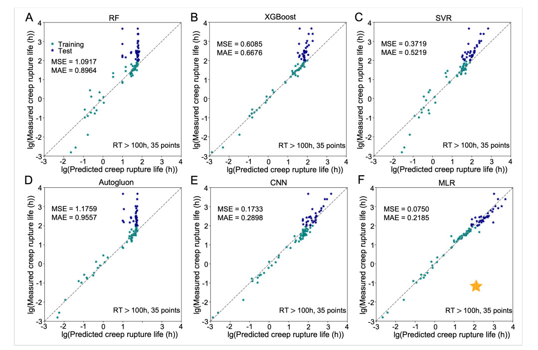
The surrogate models based on RF, XGBoost, SVR, CNN, Autogluon and MLR are trained with the training data and tested with the testing data. Figure 1 shows the extrapolation performance of the six models; the division with creep rupture life (RT)
Figure 1. Extrapolation performance of the six surrogate models on both training and testing data, the data division with RT
Reducing features for multiple-linear model
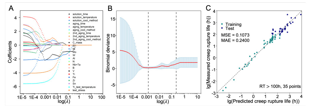
The Lasso regression is used to determine the key features. Lasso is an integration of a linear model with a regularized term. A key parameter is the coefficient (
Figure 3. Feature selection via Lasso and model performance with reduced features, the data division with RT
Figure 3B depicts the relationship between
A similar Lasso-based feature selection procedure is applied to the other six datasets with different divisions. For each dataset, we determine about ten features for an optimal linear model with the lowest error. To ensure the surrogate models and formulae can be generalized to different data division scenarios, we use the intersection of the features from the seven data sets for further modeling. The intersection has nine features: solution_time, C, Ni, Nb+Ta, V, Fe, Sn, test_temperature, and test_stress. Using these nine features, we retrain the MLR models and examine their performance for the seven data sets, as shown in Figure 4. All the models still have superior performance in both training and testing data, confirming the robustness of the nine features for extrapolation.
Figure 4. Extrapolation performance of the MLR models with nine features on the seven data divisions. (A) RT
The feature, solution_temperature, is removed due to the very small coefficient in all seven data divisions. In addition, it is noted that of the nine features, six are the contents of elements. To further simplify the MLR models, we transform the six elemental contents to a composition-based feature, the Molybdenum equivalent (
Figure 5A-G shows the performance of the new MLR models. Compared to Figure 4, there is a slight degradation in model performance. This suggests that even with three features, we can obtain accurate formulae for extrapolated prediction of creep rupture life of high-temperature titanium alloys. To demonstrate the superiority of the MLR models, we also retrain the five black-box models for comparison, as shown in Figure 6. It is found that in all seven data division scenarios, MLR models always exhibit the lowest MSE and MAE metrics. An interesting observation is that the performance of MLR consistently outperforms CNN in Figure 6, whereas this is not the case in Figure 2. This can be attributed to the fact that the CNN model can generate information-rich features by the use of convolutional kernels on high-dimensional feature space; however, the only three retained features herein may not be adequate for training a robust CNN model.
Figure 5. Extrapolation performance of the MLR models with three features on the seven data divisions. (A) RT
Simple formulae for creep rupture life prediction
The MLR algorithm assumes a linear relationship between independent and dependent variables, and the resulting models (formulae) with three features demonstrate optimal performance in extrapolated predictions. However, there may exist nonlinearity in the high-temperature titanium alloy creep data, which deserves further exploration for improved formulae. The SISSO algorithm is employed to search for better formulae, which is realized by combining the three selected basic features with arithmetic operations. Such combinations may capture the possible nonlinear patterns behind the data and provide highly accurate formulae [46].
We apply SISSO to the seven datasets and identify the corresponding optimal 2D (two variables,
The 2D and 3D SISSO formulae under different data divisions, along with the metrics for these formulas compared to the MLR models (ts means test_stress and tt means test_temperature)
| Dataset | MAE ofSISSO | MSE ofSISSO | MAE ofMLR | MSE ofMLR | |||||||
| RT100-Test | 6.7818 | -4.1975 | -4.2051 | 0.3229 | 0.4950 | 0.3941 | 0.5450 | ||||
| RT100-Test | 5.3672 | -4.6069 | -4.0322 | 0.8464 | 0.3737 | 0.5232 | |||||
| RT150-Test | 6.4416 | -4.0672 | -3.8309 | 0.3920 | 0.5616 | 0.4652 | 0.6098 | ||||
| RT150-Test | 6.2814 | -4.5942 | -3.8294 | 1.4103 | 0.4260 | 0.5772 | |||||
| RT200-Test | 6.5681 | -4.1523 | -3.8479 | 0.3233 | 0.5138 | 0.4246 | 0.5885 | ||||
| RT200-Test | 6.8009 | -4.74158 | -4.0244 | 2.1151 | 0.3162 | 0.5055 | |||||
| RT300-Test | 6.6401 | -4.2067 | -3.8421 | 0.3062 | 0.5010 | 0.4301 | 0.5926 | ||||
| RT300-Test | 6.8709 | -4.8060 | -4.0096 | 2.1381 | 0.3016 | 0.4854 | |||||
| RT400-Test | 6.7327 | -4.2581 | -3.8982 | 0.2625 | 0.4584 | 0.4696 | 0.6238 | ||||
| RT400-Test | 6.9556 | -4.8583 | -4.0598 | 2.1574 | 0.3162 | 0.4042 | |||||
| RT700-Test | 6.7670 | -4.2891 | -3.9028 | 0.2919 | 0.4946 | 0.5135 | 0.6771 | ||||
| RT700-Test | 6.9949 | -4.8912 | -4.0664 | 2.1492 | 0.3401 | 0.4608 | |||||
| RT1000-Test | 6.8457 | -4.3289 | -3.9695 | 0.2948 | 0.5130 | 0.5731 | 0.7331 | ||||
| RT1000-Test | 7.1073 | -4.9436 | -4.1695 | 2.1454 | 0.2934 | 0.4529 |
Note that although nonlinear arithmetic operations are involved in generating new features, the optimal 2D formulae we obtain contain only addition and the 3D formulae include only addition and exponentiation. Moreover, for all the seven datasets, the 2D formulae have the same
We examine the efficacy of the above formula on the seven datasets, and the model performance is compared to optimal 2D and 3D formulae (bolds in Table 1) and the MLR models [Figure 7]. Figure 7 shows that the unified formula performs similarly to those from SISSO and better than those from MLR. However, it should be pointed out that the formulae from SISSO and MLR change with different training and testing data. By contrast, the final formula in Equation (8) has a fixed form and can be preferred by the materials community.
Figure 7. Comparing the SISSO and MLR-based formulae to the "mean" formula (based on three features) on different testing datasets. (A) MSE and (B) MAE. SISSO: Sure independence screening and sparsifying operator; MLR: multiple linear regression; MSE: mean squared error; MAE: mean absolute error.
Traditionally, the TTP extrapolation methods have been used for predicting the long-term creep rupture life by fitting the measured short-term rupture life. These methods usually only consider the test_stress and test_temperature as inputs; thus, they are limited to a small subset of alloys where adequate experimental data are available. Here, in addition to test conditions, the learned formula also involves the composition-based
CONCLUSIONS
In summary, we build a variety of ML models including both black-box and white-box ones, and compare their performance in predicting the long-term creep rupture life by learning from the short-term creep rupture life data of high-temperature titanium alloys. It is found that the MLR performs much better than the other five typical black-box surrogate models, even the advanced convolutional neural networks and automated ML. Feature selection by Lasso helps to further simplify the MLR-based model, but meanwhile the accuracy degenerates. This then motivates us to use symbolic regression to establish more accurate formulae with the selected three features, the Molybdenum equivalent, the test stress and test temperature. Finally, a quite simple but unified formula is obtained for accurate creep rupture life prediction of high-temperature titanium alloys.
DECLARATIONS
Authors' contributions
Made substantial contributions to conception and design of the study and performed data analysis and interpretation: Wang P, Zhao S, Zhou C, Yuan R
Performed data acquisition and provided administrative, technical, and material support: Fan J, Tang B, Li J, Yuan R
Availability of data and materials
The data and codes are uploaded to the author's github repository: https://github.com/nwpuai4msegroup/creep-rupture-life-prediction.
Financial support and sponsorship
This work was financially supported by the National Key Research and Development Program of China (2021YFB3702604).
Conflicts of interest
All authors declared that there are no conflicts of interest.
Ethical approval and consent to participate
Not applicable.
Consent for publication
Not applicable.
Copyright
© The Author(s) 2024.
Supplementary Materials
REFERENCES
1. Zhang Z, Fan J, Tang B, et al. Microstructural evolution and FCC twinning behavior during hot deformation of high temperature titanium alloy Ti65. J Mater Sci Technol 2020;49:56-69.
2. Liu H, Wang H, Ren L, Qiu D, Yang K. Antibacterial copper-bearing titanium alloy prepared by laser powder bed fusion for superior mechanical performance. J Mater Sci Technol 2023;132:100-9.
3. Gao P, Fu M, Zhan M, Lei Z, Li Y. Deformation behavior and microstructure evolution of titanium alloys with lamellar microstructure in hot working process: a review. J Mater Sci Technol 2020;39:56-73.
4. Boyer RR. An overview on the use of titanium in the aerospace industry. Mat Sci Eng A 1996;213:103-14.
5. Wu X, Makineni SK, Liebscher CH, et al. Unveiling the Re effect in Ni-based single crystal superalloys. Nat Commun 2020;11:389.
6. Cui C, Hu BM, Zhao L, Liu S. Titanium alloy production technology, market prospects and industry development. Mater Design 2011;32:1684-91.
7. Sattar M, Othman AR, Kamaruddin S, Akhtar M, Khan R. Limitations on the computational analysis of creep failure models: a review. Eng Fail Anal 2022;134:105968.
8. Jelwan J, Chowdhury M, Pearce G. Design for creep: a critical examination of some methods. Eng Fail Anal 2013;27:350-72.
9. Barboza MJR, Neto CM, Silva CRM. Creep mechanisms and physical modeling for Ti–6Al–4V. Mat Sci Eng A 2004;369:201-9.
10. Bolton J. The potential for major extrapolation of creep rupture and creep strain data. Mate High Temp 2014;31:109-20.
11. Bolton J. Reliable analysis and extrapolation of creep rupture data. Int J Pres Ves Pip 2017;157:1-19.
12. MacLachlan DW, Knowles DM. Modelling and prediction of the stress rupture behaviour of single crystal superalloys. Mat Sci Eng A 2001;302:275-85.
13. Prasad SC, Rajagopal KR, Rao IJ. A continuum model for the anisotropic creep of single crystal nickel-based superalloys. Acta Mater 2006;54:1487-500.
14. Oruganti R, Karadge M, Swaminathan S. Damage mechanics-based creep model for 9–10% Cr ferritic steels. Acta Mater 2011;59:2145-55.
15. Zhang K, Tan JP, Sun W, Nikbin K, Tu ST. Determination of multiaxial stress rupture criteria for creeping materials: a critical analysis of different approaches. J Mater Sci Technol 2023;137:14-25.
16. Larson FR, Miller J. A time-temperature relationship for rupture and creep stresses. Trans ASME 1952;74:765-71.
17. Dyson BF. Microstructure based creep constitutive model for precipitation strengthened alloys: theory and application. Mater Sci Technol 2009;25:213-20.
18. Zhou H, Li J, Liu J, et al. Significant reduction in creep life of P91 steam pipe elbow caused by an aberrant microstructure after short-term service. Sci Rep 2024;14:5216.
19. Dang YY, Zhao XB, Yuan Y, et al. Predicting long-term creep-rupture property of Inconel 740 and 740H. Mater High Temp 2016;33:1-5.
20. Kim WG, Yin SN, Lee GG, Kim YW, Kim SJ. Creep oxidation behaviour and creep strength prediction for Alloy 617. Int J Press Ves Pip 2010;87:289-95.
21. Vladimirov IN, Reese S, Eggeler G. Constitutive modelling of the anisotropic creep behaviour of nickel-base single crystal superalloys. Int J Mech Sci 2009;51:305-13.
22. Hart GLW, Mueller T, Toher C, Curtarolo S. Machine learning for alloys. Nat Rev Mater 2021;6:730-55.
23. Shin D, Yamamoto Y, Brady MP, Lee S, Haynes JA. Modern data analytics approach to predict creep of high-temperature alloys. Acta Mater 2019;168:321-30.
24. Zhou CL, Yuan RH, Liao WJ, et al. Creep rupture life predictions for Ni-based single crystal superalloys with automated machine learning. Rare Met 2024;43:2884-90.
25. Mamun O, Wenzlick M, Sathanur A, Hawk J, Devanathan R. Machine learning augmented predictive and generative model for rupture life in ferritic and austenitic steels. Npj Mat Degrad 2021;5:20.
26. Chen C, Wang Q, Dong C, Zhang Y, Dong H. Composition rules of Ni-base single crystal superalloys and its influence on creep properties via a cluster formula approach. Sci Rep 2020;10:21621.
27. Ramprasad R, Batra R, Pilania G, Mannodi-Kanakkithodi A, Kim C. Machine learning in materials informatics: recent applications and prospects. npj Comput Mater 2017;3:54.
28. Butler KT, Davies DW, Cartwright H, Isayev O, Walsh A. Machine learning for molecular and materials science. Nature 2018;559:547-55.
29. Biswas S, Fernandez Castellanos D, Zaiser M. Prediction of creep failure time using machine learning. Sci Rep 2020;10:16910.
30. Venkatesh V, Rack HJ. A neural network approach to elevated temperature creep–fatigue life prediction. Int J Fatigue 1999;21:225-34.
31. Liu Y, Wu J, Wang Z, et al. Predicting creep rupture life of Ni-based single crystal superalloys using divide-and-conquer approach based machine learning. Acta Mater 2020;195:454-67.
32. Zhou C, Yuan R, Su B, et al. Creep rupture life prediction of high-temperature titanium alloy using cross-material transfer learning. J Mater Sci Technol 2024;178:39-47.
33. Ouyang R, Curtarolo S, Ahmetcik E, Scheffler M, Ghiringhelli LM. SISSO: a compressed-sensing method for identifying the best low-dimensional descriptor in an immensity of offered candidates. Phys Rev Mater 2018;2:083802.
34. Evans RW, Hull RJ, Wilshire B. The effects of alpha-case formation on the creep fracture properties of the high-temperature titanium alloy IMI834. J Mater Proc Technol 1996;56:492-501.
35. Zheng Z, Xiao S, Wang X, et al. High temperature creep behavior of an as-cast near-
36. Mishra H, Ghosal P, Nandy TK, Sagar PK. Influence of Fe and Ni on creep of near
37. Zheng Z, Kong F, Chen Y, Wang X. Effect of nano-
38. Li W, Chen Z, Liu J, Wang Q, Sui G. Effect of texture on anisotropy at 600 ℃ in a near-
39. Briguente LANS, Couto AA, Guimarães NM, Reis DAP, de Moura Neto C, Barboza MJR. Determination of creep parameters of Ti-6Al-4V with bimodal and equiaxed microstructure. In: Defect Diffus Forum. 2012;326-8:520–4.
40. Singh G, Satyanarayana DVV, Pederson R, Datta R, Ramamurty U. Enhancement in creep resistance of Ti–6Al–4V alloy due to boron addition. Mat Sci Eng A 2014;597:194-203.
41. Oliveira VMCA, Vazquez AM, Aguiar C, Robin A, Barboza MJR. Nitride coatings improve Ti-6Al-4V alloy behavior in creep tests. Mat Sci Eng A 2016;670:357-68.
42. Zhang Z, Fan J, Li R, et al. Orientation dependent behavior of tensile-creep deformation of hot rolled Ti65 titanium alloy sheet. J Mater Sci Technol 2021;75:265-75.
43. Omprakash CM, Satyanarayana DVV, Kumar V. Effect of primary
44. Erickson N, Mueller J, Shirkov A, et al. AutoGluon-tabular: robust and accurate automl for structured data. arXiv. [Preprint.] Mar 13, 2020 [accessed 2024 Nov 15]. Available from: https://doi.org/10.48550/arXiv.2003.06505.
45. Weiss I, Semiatin SL. Thermomechanical processing of beta titanium alloys - an overview. Mat Sci Eng A 1998;243:46-65.
46. Makke N, Chawla S. Interpretable scientific discovery with symbolic regression: a review. Artif Intell Rev 2024;57:2.
47. Yang F, Li Z, Wang Q, et al. Cluster-formula-embedded machine learning for design of multicomponent
48. Monkman FC. An empirical relationship between rupture life and minimum creep rate in creep-rupture tests. 1956. pp. 593–620. Available from: https://api.semanticscholar.org/CorpusID:222409633. [Last accessed on 15 Nov 2024.
49. McCartney M, Haeringer M, Polifke W. Comparison of machine learning algorithms in the interpolation and extrapolation of flame describing functions. J Eng Gas Turbines Power 2020;142:061009.
Cite This Article
How to Cite
Download Citation
Export Citation File:
Type of Import
Tips on Downloading Citation
Citation Manager File Format
Type of Import
Direct Import: When the Direct Import option is selected (the default state), a dialogue box will give you the option to Save or Open the downloaded citation data. Choosing Open will either launch your citation manager or give you a choice of applications with which to use the metadata. The Save option saves the file locally for later use.
Indirect Import: When the Indirect Import option is selected, the metadata is displayed and may be copied and pasted as needed.


Comments
Comments must be written in English. Spam, offensive content, impersonation, and private information will not be permitted. If any comment is reported and identified as inappropriate content by OAE staff, the comment will be removed without notice. If you have any queries or need any help, please contact us at [email protected].