

Assessing tipping-point risk in carbon dioxide removal with a network-based framework
 0
0 Graphical Abstract
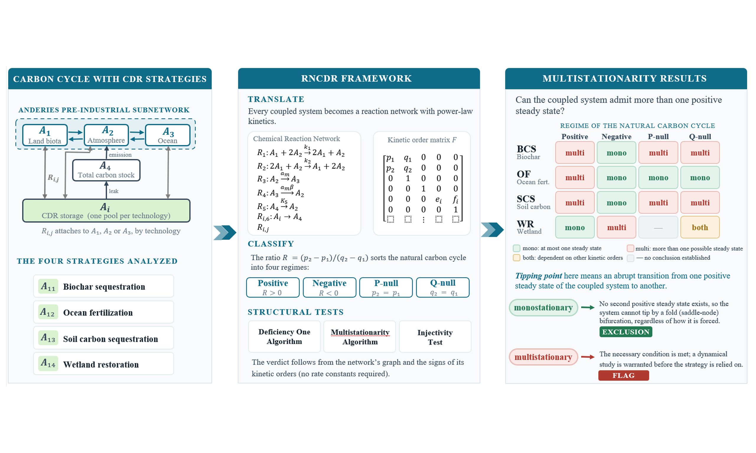
Abstract
Carbon dioxide removal (CDR) strategies are central to long-term plans for reaching carbon neutrality, and projections of their mitigation potential underpin national and global carbon accounting. How reliably a strategy delivers that potential depends on how its technology interacts with the natural carbon cycle, and in particular on whether the coupled system can settle into more than one steady state. Throughout, a tipping point means an abrupt transition from one positive steady state of the coupled system to a different one. Multiple steady states are a necessary condition for such a transition since a system with only one has no second state to move to. Such a shift would leave the strategy removing far less CO2 than projected, invalidating the carbon accounting that justified it, and recovery may be slow. Using Chemical Reaction Network Theory (CRNT), we represent four CDR strategies (biochar sequestration, ocean fertilization, soil carbon sequestration, and wetland restoration) as networks of carbon pools and the transfers between them. From the graphical and kinetic structure of each network alone, without exact rate values, we identify the conditions under which multiple steady states can exist and those under which they are excluded. For ocean fertilization, multiple steady states are guaranteed in one regime of the natural carbon cycle, provided the technology's own reaction sensitivities also meet additional conditions; outside this identified regime, the framework does not rule multistationarity out. Biochar sequestration and soil carbon sequestration share the broadest reach across the regimes in which multiple steady states can occur, reflecting shared features of their networks. Wetland restoration departs most from the others, admitting at most one steady state in a regime where the other three admit multiple. The network-level structure of a CDR system is therefore itself an assessment criterion for the reliability of projected carbon removal, and CRNT offers a parameter-minimal first screen for tipping-point risk, complementing conceptual and numerical carbon-cycle models.
Keywords


 Download PDF
INTRODUCTION
The global carbon cycle can settle into more than one steady state. This possibility, supported by a growing body of modeling evidence[1,2], is consequential because it implies the existence of climate "tipping points": thresholds beyond which the system may shift abruptly and irreversibly into a warmer equilibrium from which recovery is practically impossible[3,4,5]. Human-induced climate change may be pushing the Earth system closer to such thresholds[5,6], and the mechanisms governing these transitions remain poorly understood[7,8].
This uncertainty has direct implications for carbon dioxide removal (CDR), the family of strategies aimed at actively removing CO2 from the atmosphere as part of long-term carbon neutrality planning[9,10,11]. Projections of how much CO2 each strategy can remove over a given horizon (i.e., its mitigation potential) are a core input to national carbon budgets, Intergovernmental Panel on Climate Change (IPCC) scenario pathways, and the carbon accounting that guides long-term climate policy[9,12,13]. The existence of multiple steady states in a CDR system could have significant consequences for whether that projected potential is actually delivered. If a CDR system settles into a steady state that removes far less CO2 than projected, the carbon accounting behind its deployment no longer holds, and the broader mitigation pathway built around it may fail to meet its emissions targets. Moreover, abrupt transitions between steady states would make this risk especially difficult to anticipate or quickly recover from, since the shift could occur faster than monitoring, reporting, and verification systems can detect. Yet a critical gap remains in our understanding of when and how CDR systems exhibit multiple steady states under varying environmental conditions[10,14].
Current approaches to CDR risk assessment address related but different questions. Earth system models project how the climate responds to a given deployment over time, and multi-model intercomparisons have shown that the carbon cycle does not simply retrace its path when emissions turn negative[15,16]. Integrated assessment models ask which mix of technologies is affordable under land and energy constraints, taking the removal rates themselves as given[9,17]. Life-cycle, permanence and monitoring frameworks ask whether the carbon stored at a particular site will stay there, and whether that can be verified[14,18,19]. Deployment-impact studies ask what scaling would cost in resources; recent work finds that removal at the gigatonne scale could strain energy, water and land systems across whole regions[20,21]. None of them asks a prior question: whether the coupled system of technology and carbon cycle can settle into more than one steady state at all.
Earth system models would seem the natural place to look for multiple steady states, but they are not designed for the task. They are indispensable for projecting climate trajectories and human impacts[1,22], and they achieve this by integrating the system forward in time under prescribed forcing rather than by locating the states it can settle into. Those states are seldom computed, and the slow processes that would determine them are among the least constrained by observation[2,16]. The number of steady states a coupled CDR–carbon-cycle system admits is therefore a question posed at the level of smaller and simpler models, where the steady states are well defined and open to direct study[3,7,8]. Even at that level, locating them by simulation requires sweeping a parameter space that is large and poorly constrained. A more tractable approach is needed, one that can characterize multistationarity, the property of admitting more than one positive steady state, from the structure of the system rather than from exhaustive numerical simulation.
Chemical Reaction Network Theory (CRNT) provides a framework well-suited to this purpose. Originally developed in the context of chemical kinetics, CRNT represents system components as interacting species and transfers between them as reactions governed by rate laws. When formulated with power-law kinetics, it admits a parameter-minimal analysis that relies primarily on the graphical and kinetic structure of the network, rather than precise parameter values, to identify sufficient conditions under which multiple steady states may arise. This makes the framework well-suited to systems in which parameter uncertainty is high. The carbon-cycle box models considered here are such systems. Reaction network modeling has been successfully applied to biochemical networks[23,24], ecological systems[25,26], and epidemiology[27], and its application to the carbon cycle is an active and growing area[28,29,30,31].
In this study, we apply the Reaction Network Carbon Dioxide Removal (RNCDR) framework[29] to analyze steady-state multiplicity in four CDR strategies: biochar sequestration, ocean fertilization, soil carbon sequestration, and wetland restoration. Each system is translated into a reaction network with power-law kinetics, in which carbon pools, namely land biota, atmosphere, ocean, total carbon stock, and CDR storage, play the role of interacting species, and carbon transfers between them are modeled as reactions. The resulting network structure is analyzed to identify parameter conditions under which the system may exhibit multistationarity or is guaranteed to be monostationary, admitting at most one positive steady state. This distinction is crucial: a multistationary CDR system could settle into a steady state characterized by low net CO2 removal performance, undermining its reliability as a climate mitigation tool, while a monostationary system offers more predictable and recoverable dynamics. This approach provides a practical, structure-based way to screen each of the four CDR strategies for the possibility of multistable behavior. The screen comes before any commitment to detailed numerical modeling of a specific deployment.
A screen of this kind establishes less than the language of tipping points suggests, and the distinction is worth drawing at the outset. We use tipping point throughout in a specific sense: an abrupt transition from one positive steady state of the coupled system to a different one. Thus, multiple steady states are necessary since a system admitting only one has no second state to move to. They are not sufficient. A transition also requires that at least two of those states be attractors, that the one currently occupied cease to be available as conditions drift, and that a disturbance of realistic magnitude carry the system across the basin between them. Abrupt behavior of other kinds, which does not end in a second steady state, falls outside this definition and outside what we analyze; Section "Multistationarity and tipping points: what this framework does and does not establish" provides the distinction. Whether that occurs depends on perturbation magnitude, timescale and prevailing conditions, none of which is resolved here, and the other mechanisms by which a system may tip lie outside the analysis altogether.
The two kinds of results reported below therefore differ in force. A monostationarity result is an exclusion: a system admitting a unique positive steady state across a parameter range has no second state with which one could merge and vanish, and so cannot tip by that route however it is forced. A multistationarity result is a flag rather than a diagnosis: the structural precondition is present, and the configuration warrants dynamical study before the strategy is relied upon. We retain the language of tipping-point risk throughout, since it is the concern that makes the structural question worth asking, but no result in this paper establishes that any particular deployment will tip. Section "Multistationarity and tipping points: what this framework does and does not establish" develops the distinction and states its limits.
The remainder of the paper is structured as follows. Section "THE RNCDR FRAMEWORK" presents the RNCDR framework. Section "FOUR CDR STRATEGIES AND THEIR REACTION NETWORK REPRESENTATIONS" describes the four CDR systems and their reaction network representations. Section "CONDITIONS FOR MULTISTATIONARITY IN CDR REACTION NETWORKS" establishes the multistationarity and monostationarity conditions for each system. Section "COMPARATIVE ANALYSIS AND IMPLICATIONS" presents a comparative analysis of the four systems and discusses implications for CDR risk assessment. Section "SUMMARY, CONCLUSION, AND FUTURE RESEARCH" concludes with a summary of the key findings, their broader significance for Earth system science and climate policy, and directions for future research.
THE RNCDR FRAMEWORK
The RNCDR framework, formally introduced by Fortun et al.[29], builds on and extends their earlier work[31,32]. This approach applies CRNT to model the Earth's carbon cycle and, in the most recent studies[28,30], to two carbon removal technologies, direct air capture (DAC) and direct ocean capture (DOC). The present study expands this line of work by applying the RNCDR framework to four additional CDR strategies, namely biochar sequestration, ocean fertilization, soil carbon sequestration, and wetland restoration, and by carrying out a comparative steady-state analysis across them to identify structural conditions of multistationarity that are common to, or distinctive of, each strategy.
A chemical reaction network (CRN) is a way of describing a system in terms of three ingredients: the species (the things that interact, in our case the carbon pools), the complexes (the combinations of species that appear on either side of an arrow, such as land plus atmosphere), and the reactions (the directional transfers from one complex to another, each describing a way carbon moves through the system). Together, these define the structure of the network. Each reaction is assigned a rate function describing how fast it proceeds, and the collection of these rates gives the dynamics of the system. In this study, the rate functions take the form of power-law kinetics, a flexible class of rate laws that can approximate a wide range of biogeochemical processes. Precise definitions are provided in Supplementary Section 1.
In this framework, the global carbon cycle is modeled as a CRN in which carbon moves among five interconnected pools: land biota (
Every RNCDR system is assembled from three components: the Anderies pre-industrial subnetwork, the fossil fuel emission reaction, and the CDR carbon storage. Figure 1 provides an overview of how these three components combine to form an RNCDR system. The Anderies pre-industrial subnetwork (Component 1) tracks the natural carbon cycle among land biota, the atmosphere, and the ocean. The fossil fuel emission reaction (Component 2) introduces the total carbon stock and the transfer of carbon from this stock to the atmosphere. The CDR carbon storage (Component 3) introduces a storage pool
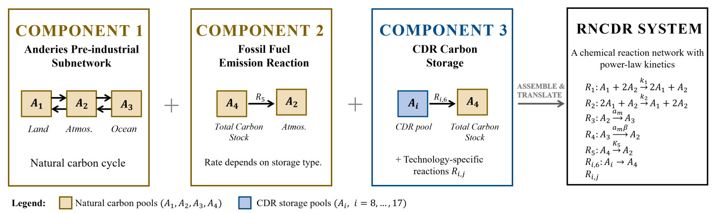
Figure 1. Structure of an RNCDR system. Every RNCDR model is assembled from three components: the Anderies pre-industrial subnetwork representing the natural carbon cycle among land biota (
Building an RNCDR system from three components
The foundation of every RNCDR model is the Anderies pre-industrial subnetwork, which captures the natural carbon cycle among land (
The model tracks carbon transfers among three pools, namely land (
The model is formulated as a generalized mass action (GMA) system[34,35,36]. This is an ordinary differential equation (ODE) system in which each carbon transfer is individually approximated by a power-law term via Taylor linearization in logarithmic coordinates, with a positive sign for incoming transfers and a negative sign for outgoing transfers. The resulting CRN representation is dynamically equivalent to the original ODE system. The power-law approximation is summarized in Table 1, and the resulting ODE system, due to the carbon-cycle model of Anderies et al.[3] in the power-law representation of Fortun et al.[32], is:
where the kinetic orders
| Carbon transfer | Rate constant | Power-law kinetic |
The CRN representation of the subnetwork consists of four reactions:
Reactions
The industrial carbon cycle introduces the total carbon stock
which transfers carbon from the total carbon stock directly into the atmosphere through the combustion of its geological component. The rate function
Each CDR technology introduces one additional storage pool
where
Notation for CDR-specific storage species
| Symbol | CDR technology |
| Bioenergy with Carbon Capture and Storage (BECCS)[29] | |
| Direct Air Capture (DAC)[30] | |
| Enhanced Weathering (EW)[39] | |
| Biochar[40] | |
| Ocean Fertilization (OF)[41] | |
| Soil Carbon Sequestration (SCS)[42] | |
| Wetland Restoration (WR)[43] | |
| Afforestation/Reforestation (AR)[44] | |
| Ocean Alkalinization (OA)[45] | |
| Direct Ocean Capture (DOC)[28] |
Characterizing the storage with $$ \lambda_i $$ $$ \mu_i $$
Not all CDR technologies store carbon in the same way. Two parameters characterize the output of each technology:
●
Parameter values
| Technology | Physical storage | |||
| BECCS ( | CO2 injected into geological stock | 1 | 0 | 0 |
| DAC ( | CO2 injected into geological stock | 1 | 0 | 0 |
| EW ( | Rock spread on beaches/fields | 1 | 1 | 1 |
| Biochar ( | Biocharcoal in soil (0.5), biofuel in geostock (0.5) | 1 | 0.5 | 0.5 |
| OF ( | Deep ocean | 1 | 0 | 0 |
| SCS ( | Soil (microbial enhancement) | 0.01 | 0 | 0.99 |
| WR ( | Wetland floor | 0.01 | 0.9 | 0.999 |
| AR ( | Sequence of trees and soil | 0.5 | 0 | 0.5 |
| OA ( | Deep ocean | 1 | 1 | 1 |
| DOC ( | CO2 injected into geological stock | 1 | 0 | 0 |
●
Only organic carbon held in the geological reserve can be released by fossil fuel combustion. The emittable fraction of captured carbon is therefore
These parameters (see Table 3) are best understood as relative estimates rather than fixed empirical quantities; they allow the model to explore system behavior under different assumptions and can be recalibrated as real-world data become available.
Because these values are nominal rather than measured, it is worth being explicit about how far the results depend on them. The two parameters enter the analysis only through the single combination
the fraction of CDR storage withheld from emission, which, together with the positive steady state about which (5) is linearized, determines the emission kinetic orders
Connecting storage to the atmosphere through the emission reaction
The emission reaction
where the term
where the kinetic orders satisfy
These three conditions have clear physical interpretations:
Encoding the kinetics in the kinetic order matrix
The power-law kinetics of the entire RNCDR system is encoded in the kinetic order matrix F, whose entry
The rows for
Classifying RNCDR systems
The dynamic behavior of an RNCDR system is strongly shaped by the properties of its Anderies subnetwork. Following[31], we classify Anderies systems – and by extension, RNCDR systems[29]– according to the ratio
which compares how much respiration and photosynthesis differ in their influence on land biota versus atmosphere. The kinetic orders
● Positive class (
● Negative class (
● P-null class (
● Q-null class (
These classes characterize the dynamic behavior of the Anderies subnetwork in isolation. Once the Anderies subnetwork is embedded in an RNCDR system, the addition of the fossil fuel emission reaction and the CDR-specific reactions can change the steady-state behavior: a class that is monostationary at the Anderies level need not remain so for the full RNCDR system, and the propositions in Section "CONDITIONS FOR MULTISTATIONARITY IN CDR REACTION NETWORKS" make this explicit for each of the four CDR strategies analyzed.
Note the asymmetry in these definitions: the P-null class arises when the numerator of R vanishes (i.e.,
Therefore, an RNCDR kinetic system for a single CDR technology consists of five species (
Figure 2 summarizes how the RNCDR framework is applied in practice. The analysis proceeds in five steps: (1) selecting a CDR strategy; (2) parametrizing its storage through

Figure 2. The RNCDR analysis workflow. Each CDR strategy is screened for tipping-point risk through five sequential steps: selecting the strategy, parametrizing its storage, representing it as a chemical reaction network, classifying the Anderies subnetwork, and testing for multistationarity or monostationarity. The framework relies on the graphical and kinetic structure of the network rather than precise rate constants.
The key question the framework is designed to answer is: Under what conditions can a CDR system settle into more than one steady state, and therefore become vulnerable to a tipping point that would compromise the carbon removal it was designed to deliver? As explored in the subsequent sections, the answer depends critically on the class (positive, negative, or null) of the underlying Anderies subnetwork, and on the structural features of the CDR-specific reactions, including their kinetic orders and the resulting network deficiency. This provides a basis for screening CDR strategies for carbon-accounting risk before their projected mitigation potential is committed to in deployment plans or long-term climate policy.
Multistationarity and tipping points: what this framework does and does not establish
Throughout this paper, multistationarity means the existence of more than one positive steady state, and monostationarity means that at most one exists. Relating these to tipping requires care, because tipping is not a single phenomenon. We take a tipping point to be an abrupt transition from one positive steady state to a different one, and on that definition multistationarity is necessary: the destination state must exist. The definition is narrower than the term as used in the wider literature. In the classification of Ashwin et al.[46], now standard in this field[47], a system may tip through a bifurcation of a quasi-static attractor as a control parameter drifts (B-tipping), through noise carrying it out of a basin of attraction (N-tipping), or through failing to track a moving attractor when that parameter changes too quickly (R-tipping). Each can end somewhere other than a second steady state, in a limit cycle or an excitable excursion, and R-tipping in particular can occur in systems whose steady state is unique and globally attracting[46,48]. Those cases lie outside our definition, and outside what the framework addresses.
Within that definition, what the framework establishes can be stated exactly. A system admitting at most one positive steady state throughout a parameter range has no second state to move to, and so cannot undergo a transition of this kind however it is forced. That is a conclusion about the dynamics obtained from the structure of the network alone, and it holds whichever mechanism might otherwise have driven the transition. The best studied of these is the fold, or saddle-node, bifurcation, in which two steady states merge and annihilate as a slowly varying control passes a threshold; monostationarity excludes it directly, since the merging requires two states to begin with.
Nor does the argument require the system to be at rest. A system need not settle into a steady state for the number of steady states to matter, since the steady states and their stability determine which transitions are available to it. The results below should accordingly be read asymmetrically. A monostationarity result is an exclusion: under the stated kinetic-order conditions the model cannot support multiple positive steady states, and so cannot support a transition between them at all. A multistationarity result is a flag rather than a diagnosis: the necessary condition is met, and a dynamical study of the configuration is warranted before the strategy is relied upon. Establishing that a transition would actually occur requires stability, basin geometry, perturbation magnitude and timescale, none of which is determined here, and we retain the language of tipping-point risk only because it is the concern that makes the structural question worth asking.
FOUR CDR STRATEGIES AND THEIR REACTION NETWORK REPRESENTATIONS
This section presents the reaction network representations of the four CDR strategies analyzed in this study --- biochar sequestration, ocean fertilization, soil carbon sequestration, and wetland restoration --- together with the box models used to represent each system, their corresponding RNCDR reaction network translation, and the kinetic order matrices encoding their dynamics. Each system extends the RNCDR framework of Section "THE RNCDR FRAMEWORK" by specifying the CDR storage species
The four strategies were chosen to span the ways in which CDR systems physically hold carbon and the settings in which they are deployed, rather than to sample a single class of technology. Biochar sequestration stores carbon as a solid, thermochemically stabilized product applied to agricultural soil. Ocean fertilization stores it in the deep ocean by way of the marine biological pump. Soil carbon sequestration stores it as soil organic matter maintained by land management practice. Wetland restoration stores it in waterlogged sediment, where anoxia suppresses decomposition[43]. The four therefore differ in the medium that holds the carbon, in how long it is held, and in how it is lost: biochar by slow oxidation of the applied char[40,49], ocean carbon by overturning circulation returning it to the surface, soil carbon by tillage or a reversal of land use, and wetland carbon by drainage[19].
They differ likewise in deployment setting and maturity. Biochar is applied in a distributed way on agricultural land and is already produced commercially. Soil carbon sequestration operates over large areas of existing farmland at low cost per hectare, but its gains saturate as soils approach a new equilibrium and are difficult to verify[42,50]. Wetland restoration is undertaken at the scale of individual coastal and inland sites, usually alongside biodiversity and flood-protection objectives. Ocean fertilization requires no land at all, but its efficacy is contested and it is restricted under international marine agreements. The set thus ranges from a commercially delivered engineered product, through two forms of land and ecosystem management, to an open-ocean intervention that remains experimental.
This spread is what makes the four informative within the RNCDR framework, since permanence and reversibility enter the model directly through
The remaining technologies in Table 2 are excluded for specific reasons. Direct air capture, direct ocean capture and bioenergy with carbon capture and storage have already been analyzed within this framework[28,29,30], and all three store captured CO2 by injection into geological formations, so including them here would duplicate both the published analysis and a storage mechanism already covered. Enhanced weathering and ocean alkalinization store carbon geochemically, as dissolved bicarbonate and carbonate rather than as organic matter, and the carbon follows a long multi-step path from mineral grain through soil solution and rivers to the ocean; representing that path faithfully would require pools beyond the five used here, and we therefore treat the two together as the natural next case. Afforestation and reforestation store carbon in standing biomass and soil on a route close to that of biochar, and would add no new coverage of the storage-parameter space, since
Biochar sequestration
Biochar sequestration, hereafter referred to as the BCS system, involves incorporating carbon-rich biochar into soils to enhance long-term carbon storage[40]. Biochar is produced from biomass through pyrolysis, a process of burning organic material in an oxygen-limited environment, creating a stable, carbon-rich material that resists decomposition. In the RNCDR framework, biochar storage is represented by
The box model is shown in Figure 3. The BCS system involves five carbon pools: land biota (
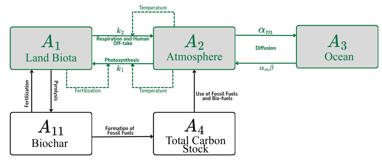
Figure 3. Box model of the biochar sequestration system. The green-outlined pools and reactions (
Together with the four Anderies reactions
The row for
Ocean fertilization
Ocean fertilization, hereafter referred to as the OF system, seeks to stimulate the growth of marine phytoplankton to enhance the oceanic uptake of CO2[41]. The process introduces nutrients such as iron to the ocean surface, inducing phytoplankton blooms that absorb atmospheric carbon into their biomass. When the phytoplankton die, their biomass sinks to the deep ocean where the carbon is stored for a long period of time. The efficacy of ocean fertilization is contested. Field experiments have generally found that only a small and highly variable fraction of the carbon fixed in a bloom reaches the deep ocean, and estimates of the cost per tonne removed span roughly two orders of magnitude, driven largely by uncertainty in that export efficiency[41,51]. Deployment beyond legitimate scientific research has been restricted since 2008 by resolution of the parties to the London Convention and Protocol, an approach codified in a 2013 amendment to the London Protocol that has not yet entered into force[41]. We retain it here as a modeling case rather than as an endorsement: it continues to appear in CDR portfolio inventories, and it is the analytically distinctive member of our set, being the only one of the four whose emission reaction reduces exactly to linear mass action. In the RNCDR framework, OF storage is represented by the separate pool
The box model is shown in Figure 4. The OF system involves five carbon pools: land biota (
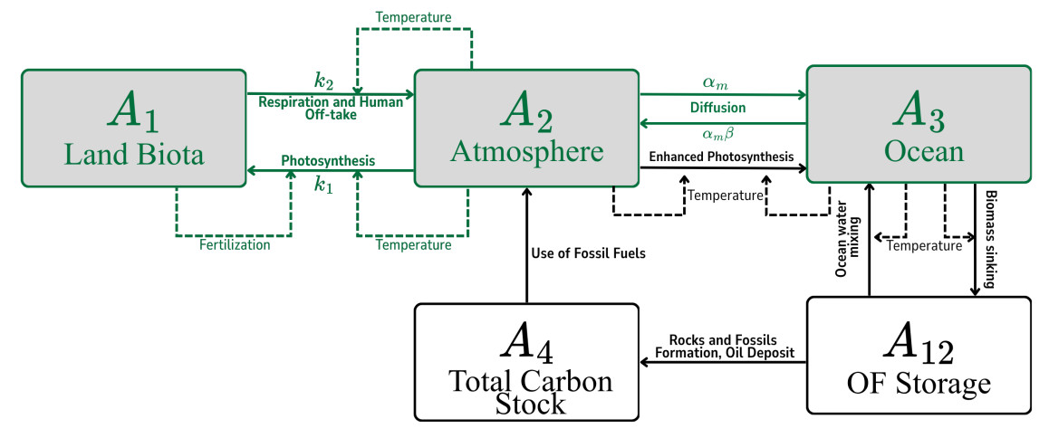
Figure 4. Box model of the OF system. As in Figure 3, the green-outlined portion reproduces the Anderies subnetwork.
Together with
The row for
Soil carbon sequestration
Soil carbon sequestration, hereafter referred to as the SCS system, aims to increase the organic carbon content of agricultural and natural soils through various land management practices[42]. Carbon from the atmosphere is absorbed by plants through photosynthesis and stored in the soil as soil organic carbon. Practices such as cover cropping, crop rotation, and reduced tillage are used to increase the rate at which carbon is added to the soil while decreasing the rate at which it is lost through decomposition. In the RNCDR framework, SCS storage is represented by
The box model is shown in Figure 5. The SCS system involves five carbon pools: land biota (
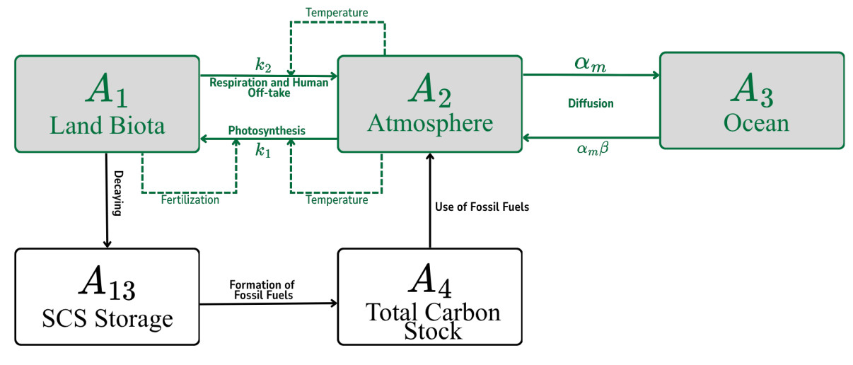
Figure 5. Box model of the SCS system. As in Figure 3, the green-outlined portion reproduces the Anderies subnetwork.
Together with
The row for
Wetland restoration
Wetland restoration, hereafter referred to as the WR system, leverages the natural carbon sequestration capacity of wetland ecosystems[43]. Wetlands are ecosystems where plants and soil are submerged in water; they can capture large amounts of CO2 from the atmosphere and store it in soils for hundreds or even thousands of years. In the RNCDR framework, WR storage is represented by
The box model is shown in Figure 6. The WR system involves five carbon pools: land biota (
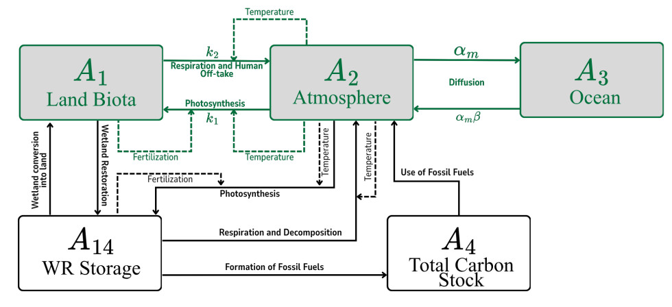
Figure 6. Box model of the WR system. As in Figure 3, the green-outlined portion reproduces the Anderies subnetwork.
Together with
The WR system has the largest kinetic order matrix among the four systems, reflecting its greater complexity. The rows for
CONDITIONS FOR MULTISTATIONARITY IN CDR REACTION NETWORKS
Having established the RNCDR representations of the four CDR systems, we now present the conditions under which each system may exhibit multistationarity, the capacity to admit more than one positive steady state, or is guaranteed to be monostationary, settling into at most one. Recall from Section "THE RNCDR FRAMEWORK" that the dynamic behavior of the underlying Anderies subnetwork is organized by the ratio
The analysis proceeds by applying two complementary tools to each CRN representation. A key structural index that determines which tools are applicable is the deficiency of the network. The deficiency is a non-negative measure that quantifies the degree of "linear independence" among a network's reactions[52]. A deficiency of zero represents the highest level of linear independence consistent with the network's directed graph structure. Conversely, a higher deficiency indicates a lower degree of linear independence, indicating greater complexity in the network structure. As shown in Supplementary Section 3, the BCS and SCS systems have deficiency
To establish monostationarity, we apply the injectivity test of Wiuf and Feliu[53,54], which uses a computational approach and Maple script to determine whether the determinant of the matrix
Proposition 1 (Biochar Sequestration). The following hold for the BCS system:
(i) Positive class. If
(ii) Negative class. If
(iii) P-null class. The system is multistationary.
(iv) Q-null class. The system is multistationary.
The conditions
Proposition 2 (Ocean Fertilization). The following hold for the OF system:
(i) Positive class. If
(ii) Negative class. If
(iii) Q-null class. If
(iv) P-null class. If
A notable feature of the OF system is that, since
Proposition 3 (Soil Carbon Sequestration). The following hold for the SCS system:
(i) Positive class. If
(ii) Negative class. If
(iii) Q-null class. If
(iv) P-null class. If
Despite differences in their underlying physical processes, the SCS and BCS systems exhibit the same multistationarity profile across Anderies classes: both admit multistationary subsets in the positive, P-null, and Q-null classes, with monostationarity guaranteed only in the negative class under appropriate sign conditions. The two systems therefore share the broadest reach of multistationarity across Anderies classes among the four strategies analyzed.
Both BCS and SCS admit the DOA, which identifies parameter conditions under which multiple steady states exist in the positive, P-null, and Q-null classes for these networks. The DOA's applicability follows from the deficiency-one structure of both networks together with the specific kinetic-order pattern in which the CDR storage species (
Proposition 4 (Wetland Restoration) The following hold for the WR system:
(i) Positive class. If
(ii) Negative class. If
(iii) Q-null class.
(a) If
(b) If
The WR system exhibits the most nuanced multistationarity behavior among the four systems. Unlike the BCS, OF, and SCS systems, where multistationarity arises in the positive class, the WR system is monostationary in the positive class and multistationary in the negative class. This is a consequence of the richer network structure of the WR system, which involves bidirectional transfers between the atmosphere and WR storage mediated by additional kinetic orders
This result also depends on the storage parameterization in a way the others do not. Proposition 4(i) requires
This reversal of the positive- and negative-class behavior carries an implication for how WR might be represented in larger climate models. Models that capture the natural carbon cycle but treat the wetland–atmosphere interaction as a one-way flux to a storage pool would correspond, in the RNCDR framework, to a system without the bidirectional coupling encoded in
COMPARATIVE ANALYSIS AND IMPLICATIONS
Comparative analysis
Table 4 summarizes the steady-state capacity of the four CDR systems by Anderies class. The results established in Section "CONDITIONS FOR MULTISTATIONARITY IN CDR REACTION NETWORKS" are sufficient conditions. They identify specific parameter combinations under which a system is guaranteed to contain multistationary or monostationary subsets. They do not preclude other behaviors under different parameter combinations. The Anderies class, defined by the signs of
Visual summary of steady-state capacity of the four CDR systems by Anderies class
| System | Positive | Negative | P-null | Q-null |
| BCS | MSa | monob | MSa | MSa |
| OF | MSa | monob | monob | monob |
| SCS | MSa | monob | MSa | MSa |
| WR | monob | MSa | — | both |
It bears emphasis that a system belonging to the positive class is not guaranteed to be multistationary for all parameter combinations; rather, there exist specific parameter regions within that class where multiple positive steady states can occur. Establishing whether a particular real-world deployment falls within such a region requires empirical estimation of the kinetic orders, a potential research direction discussed in Section "SUMMARY, CONCLUSION, AND FUTURE RESEARCH".
With this caveat in mind, the following observations can be made. The OF system stands alone in having multistationary subsets identified exclusively in the positive Anderies class. This pattern does not mean the Anderies class alone determines the outcome for OF: as for the other three systems, every case in Proposition 2 additionally requires sign conditions specific to the OF reactions themselves. The BCS and SCS systems share the same multistationarity profile: multistationary subsets have been identified in the positive class and also in both the P-null and Q-null classes, with monostationarity guaranteed only in the negative class. This shared profile follows from shared structural properties of the two networks. Both are deficiency-one networks in which the CDR-specific reactions extend the natural carbon cycle without directly modulating its rates. For both, the DOA identifies parameter conditions under which multistationarity arises in the positive, P-null, and Q-null classes. The WR system departs most significantly from the others: monostationary subsets have been identified in the positive class and multistationary subsets in the negative class, with the Q-null class containing both monostationary and multistationary subsets depending on the sign of
These differences can be understood in terms of the structural features of each CDR system. Among the four, the OF system is the deficiency-two network in which the CDR-specific reactions do not directly modulate the rates of the natural carbon cycle reactions
Implications for CDR risk assessment
The findings of this study have three important implications for CDR risk assessment and carbon neutrality planning.
First, the Anderies class of the natural carbon cycle should be treated as a prerequisite screening criterion in CDR risk assessment. Before evaluating any specific technology, policymakers and modelers could check whether the background carbon cycle is in a positive, negative, or null class. For the OF system, multistationary subsets were identified in the positive Anderies class alone. That determination is not by itself sufficient, however: Proposition 2 additionally requires sign conditions on the OF-specific kinetic orders
Second, the four systems demonstrate that the network-level structure of a CDR system is itself risk-relevant, and that this structure can take qualitatively different forms. The OF system illustrates a deficiency-two case in which the CDR-specific reactions do not directly modulate the natural carbon cycle reactions; even so, the system's steady-state behavior is not organized by the Anderies class alone, since realizing the multistationarity it flags additionally requires sign conditions specific to the OF reactions (Proposition 2). The BCS and SCS systems illustrate the deficiency-one case in which the CDR-specific reactions extend the natural carbon cycle without modulating its rates, and the DOA identifies parameter conditions under which multistationarity arises in classes that would be monostationary at the Anderies level. The WR system illustrates the case in which bidirectional coupling between the storage pool and the atmosphere, encoded in the kinetic orders
Third, the parameter-minimal nature of the RNCDR framework means that the conclusions above hold without requiring precise knowledge of rate constants. The framework relies primarily on the graphical and kinetic structure of the network, rather than on specific parameter values, making it particularly well-suited to systems in which parameter uncertainty is high and exhaustive numerical simulation is impractical. As a practical example, the sign conditions on
Relation to other CDR assessment methods
Table 5 places the RNCDR framework alongside the other families of methods used to assess CDR strategies. The framework is not an alternative to numerical simulation. It is a screen applied before simulation, and the asymmetry noted in Section "Multistationarity and tipping points: what this framework does and does not establish" defines its practical scope: a guaranteed monostationarity result excludes a configuration from further dynamical investigation, whereas a multistationarity result identifies where such investigation is warranted. Its computational cost is negligible by comparison, because the propositions follow from the structure of the network rather than from integrating the governing equations.
Families of methods used in CDR assessment, and the question each answers
| Approach | Question answered | Requirements | Cannot establish |
| Earth system models[15,16] | Transient response to prescribed CDR forcing | Full parameterization; high-performance computing | Equilibrium multiplicity |
| Integrated assessment models[9,17] | Portfolio composition under economic constraints | Cost and land-use data | Carbon-cycle dynamics |
| Reduced-complexity box models[3,7,8] | Trajectories and equilibria of aggregated pools | Rate constants | Generality across parameter values |
| Permanence and verification frameworks[18,19] | Durability and auditability of a deployment | Site-level monitoring | System-level feedbacks |
| RNCDR (this work) | Whether more than one positive steady state can exist | Network structure and kinetic-order signs | Stability, basins, timescales |
Limitations
Several limits bear on how these results should be used. The conditions established in Section "CONDITIONS FOR MULTISTATIONARITY IN CDR REACTION NETWORKS" are sufficient rather than necessary. They identify parameter regions in which multistationarity or monostationarity is guaranteed, but they do not partition the parameter space, and behavior outside those regions is not determined by the present analysis. Nor does the existence of multiple positive steady states imply that more than one of them is an attractor. Establishing bistability would require a linearized stability analysis that we do not perform, which is the distinction drawn in Section "Multistationarity and tipping points: what this framework does and does not establish": multistationarity is a structural precondition for one tipping mechanism rather than a demonstration of tipping. The scope is also narrower than the word "tipping" suggests. We take a tipping point to be an abrupt transition from one positive steady state to another, and the results speak only to that. Abrupt behavior that ends somewhere else (e.g., in a limit cycle) lies outside the definition; so does rate-induced tipping in a system with a unique steady state. This is not a remote concern for the systems studied here. The compost-bomb instability, in which soil carbon is released explosively above a critical rate of warming, is a rate-induced phenomenon. It arises in a soil-carbon model whose steady state is unique and globally attracting[48,56]. A monostationarity result for the SCS system would not exclude behavior of that kind.
The representation is also highly aggregated. It has five carbon pools, no spatial resolution and no explicit temperature state variable, so climate feedbacks enter only through the kinetic orders rather than as dynamical variables in their own right.
Two sets of parameters remain unconstrained by observation. The Anderies classification depends on
Finally, the analysis covers single-technology deployments only; portfolios of simultaneously deployed strategies are not treated here, although the framework accommodates them. And a steady-state analysis is silent on time. It says nothing about how long a transition between states would take, which is precisely the quantity that determines whether monitoring, reporting and verification systems could detect one.
SUMMARY, CONCLUSION, AND FUTURE RESEARCH
This study applied the RNCDR framework to analyze the steady-state multiplicity of four CDR strategies, namely biochar sequestration, ocean fertilization, soil carbon sequestration, and wetland restoration, by translating each system into a chemical reaction network with power-law kinetics and examining the graphical and kinetic structure of the resulting networks. The analysis identified sufficient conditions under which each system may exhibit multistationarity or is guaranteed to be monostationary, without requiring precise knowledge of rate constants. The key findings are summarized below.
● Among the four systems, OF is the one whose multistationary subsets are confined to a single Anderies class, the positive class (
● The BCS and SCS systems share the broadest reach of multistationarity across Anderies classes among the four strategies analyzed. Both exhibit multistationary subsets in the positive, P-null, and Q-null classes, with monostationarity guaranteed only in the negative class under appropriate sign conditions. This shared profile is a consequence of shared structural properties: both BCS and SCS are deficiency-one networks in which the CDR-specific reactions extend the natural carbon cycle without directly modulating its rates, and the DOA identifies parameter conditions under which multistationarity arises in classes that would be monostationary at the level of the Anderies subnetwork in isolation.
● The WR system exhibits the most parameter-dependent multistationarity behavior among the four systems analyzed. In contrast to the BCS, OF, and SCS systems, the WR system is monostationary in the positive Anderies class and multistationary in the negative class. The Q-null class contains both monostationary and multistationary subsets, depending on the sign of
● The structural design of a CDR system is itself a risk-relevant parameter, and it can take qualitatively different forms across CDR strategies. The four systems analyzed here span a range from a deficiency-two network with no direct modulation of the natural cycle (OF), to deficiency-one networks whose CDR-specific reactions extend the natural cycle without modulating its rates while admitting multistationarity in additional classes through the conditions identified by the DOA (BCS and SCS), to a deficiency-two network with bidirectional coupling between the storage pool and the atmosphere (WR). Each of these forms produces a distinct multistationarity profile across Anderies classes, demonstrating that the network-level structure of a CDR system can either introduce or suppress tipping-point risk in ways that are not predictable from the Anderies subnetwork class alone.
● The RNCDR framework provides a structure-based route to screening for multistationarity, which is a necessary condition for an abrupt transition between steady states. By relying on the graphical and kinetic structure of the network rather than precise parameter values, the framework can characterize multistationarity conditions across all four CDR systems without exhaustive numerical simulation. The sign conditions on
For Earth system science, this study demonstrates that CRNT offers a tractable and systematic complement to conceptual and numerical carbon-cycle modeling for the analysis of steady-state multiplicity, and hence of one structural precondition for tipping-point behavior. In this framework, carbon pools are represented as interacting components and carbon transfers as reactions, and the question of whether the system can settle into more than one equilibrium is answered from the structure of these interactions rather than from numerical simulation. The RNCDR framework identifies structural drivers of multistationarity from the graphical and kinetic structure of simple heuristic box models, complementing the insights available from high-dimensional computational models. The framework is designed to accommodate other CDR technologies and portfolios of simultaneously deployed strategies, as noted in Section "Limitations", though demonstrating this extensibility remains a direction for future work.
For climate policy, the findings underscore that the reliability of a CDR strategy as a climate mitigation tool cannot be assessed independently of the dynamic regime of the natural carbon cycle into which it is deployed. The natural carbon cycle can operate in qualitatively different regimes, characterized here by the Anderies class, which determines whether the system is capable of settling into more than one equilibrium carbon distribution. A CDR system deployed into a multistationary regime may settle into a steady state characterized by low net CO2 removal performance, undermining the carbon accounting assumptions underlying its deployment. The results suggest that a basic characterization of this background regime, through estimation of how photosynthesis and respiration respond to changes in carbon pool sizes, should be treated as a prerequisite screening step in CDR risk assessment, prior to the evaluation of any specific technology. Furthermore, the structural design of CDR technologies, specifically the nature of the feedback between the CDR storage pool and the natural carbon cycle, should be recognized as a risk-relevant design parameter in the development and evaluation of CDR deployment strategies. Aligning these findings with IPCC-style scenario analyses could provide further insights into the role of each CDR strategy in achieving long-term mitigation targets and inform the prioritization of technologies in national and global climate action plans[12].
Several directions for future research emerge from this study. Empirical validation of the kinetic order conditions identified here will be essential to strengthen the credibility and applicability of the results. In particular, estimating the kinetic orders
Extending the framework to portfolios of multiple CDR technologies deployed simultaneously is another important direction. The RNCDR framework is designed to accommodate such combinations, and analyzing the multistationarity behavior of CDR portfolios could reveal synergies or trade-offs that are not apparent from single-technology analyses. One case is of particular interest. BCS and SCS have multistationarity broadly distributed across Anderies classes, whereas that of OF is anchored more narrowly to a single class. Whether combining the two kinds reduces the overall tipping-point risk of a portfolio is an open question.
Finally, the model outcomes could be aligned with IPCC-style scenario analyses[12]. Doing so would give insight into the role of each CDR strategy in meeting long-term mitigation targets, and would inform how technologies are prioritized in national and global climate action plans.
DECLARATIONS
Authors' contributions
Conceptualization: Fortun, N. T.; Lao, A. R.; Mendoza, E. R.; Razon, L. F.
Methodology: Aguilar, C. J. M.; Aquino, S. A. L.; Candido, J. L. U.; Fortun, N. T.; Lao, A. R.; Mendoza, E. R.; Nocum, K. P.; Pelagio, M. E. D.; Razon, L. F.
Formal analysis, investigation, software, writing - original draft: Aguilar, C. J. M.; Aquino, S. A. L.; Candido, J. L. U.; Pelagio, M. E. D.
Visualization: Aguilar, C. J. M.; Aquino, S. A. L.; Candido, J. L. U.; Fortun, N. T.; Pelagio, M. E. D.
Supervision: Catibog, J. M.; Fortun, N. T.; Lao, A. R.; Magpantay, D. M.; Mendoza, E. R.; Nocum, K. P.; Razon, L. F.
Project administration: Fortun, N. T.; Nocum, K. P.
Funding acquisition: Catibog, J. M.; Magpantay, D. M.; Nocum, K. P.
Validation, writing - review and editing: Candido, J. L. U.; Aguilar, C. J. M.; Aquino, S. A. L.; Pelagio, M. E. D.; Fortun, N. T.; Nocum, K. P.; Catibog, J. M.; Magpantay, D. M.; Lao, A. R.; Razon, L. F.; Mendoza, E. R.
Availability of data and materials
The original contributions presented in this study are included in the article/Supplementary Materials. Further inquiries can be directed to the corresponding author.
AI and AI-assisted tools statement
During the preparation of this manuscript, the AI tool Claude (Anthropic; versions Claude Opus 4.7, released 2026-04-16, and Claude Opus 5, released 2026-07-24) was used solely for language editing and improving the readability of portions of the manuscript. The tool did not influence the study design, data collection, analysis, interpretation, or the scientific content of the work. All authors take full responsibility for the accuracy, integrity, and final content of the manuscript.
Financial support and sponsorship
Aguilar, C. J. M.; Aquino, S. A. L.; Candido, J. L. U.; and Pelagio, M. E. D. gratefully acknowledge the Department of Science and Technology–Science Education Institute (DOST–SEI), Philippines, for support through the Science and Technology Regional Alliance of Universities for National Development (STRAND) graduate scholarship program. Catibog, J. M.; Magpantay, D. M.; and Nocum, K. P. gratefully acknowledge Batangas State University, The National Engineering University (BatStateU–TNEU) for financial support in conducting this research.
Conflicts of interest
All authors declared that there are no conflicts of interest.
Ethical approval and consent to participate
Not applicable.
Consent for publication
Not applicable.
Copyright
© The Author(s) 2026.
Supplementary Materials
REFERENCES
1. Bonan, G. B.; Doney, S. C. Climate, ecosystems, and planetary futures: the challenge to predict life in earth system models. Science 2018, 359, eaam8328.
3. Anderies, J. M.; Carpenter, S. R.; Steffen, W.; Rockström, J. The topology of non-linear global carbon dynamics: from tipping points to planetary boundaries. Environ. Res. Lett. 2013, 8, 044048.
4. Lenton, T. M.; Held, H.; Kriegler, E.; et al. Tipping elements in the earth's climate system. Proc. Natl. Acad. Sci. USA. 2008, 105, 1786-93.
5. Rockström, J.; Steffen, W.; Noone, K.; et al. Planetary boundaries: exploring the safe operating space for humanity. Ecol. Soc. 2009, 14, art32.
6. Armstrong McKay, D. I.; Staal, A.; Abrams, J. F.; et al. Exceeding 1.5℃ global warming could trigger multiple climate tipping points. Science 2022, 377, eabn7950.
7. Mills, B. J. W.; Tennenbaum, S.; Schwartzman, D. Exploring multiple steady states in earth's long-term carbon cycle. Am. J. Sci. 2021, 321, 1033-44.
8. Zhu, F.; Rose, B. E. J. Multiple equilibria in a coupled climate–carbon model. J. Clim. 2023, 36, 547-64.
9. Chiquier, S.; Gurgel, A.; Morris, J.; Chen, Y. H.; Paltsev, S. Integrated assessment of carbon dioxide removal portfolios: land, energy, and economic trade-offs for climate policy. Environ. Res. Lett. 2025, 20, 024002.
10. Keller, D. P.; Lenton, A.; Littleton, E. W.; Oschlies, A.; Scott, V.; Vaughan, N. E. The effects of carbon dioxide removal on the carbon cycle. Curr. Clim. Change. Rep. 2018, 4, 250-65.
11. Morrow, D. R.; Thompson, M. S.; Anderson, A.; et al. Principles for thinking about carbon dioxide removal in just climate policy. One. Earth. 2020, 3, 150-53.
12. Shukla, P. R.; Skea, J.; Reisinger, A.; et al. Climate change 2022 - mitigation of climate change. In Proceedings of the Contribution of Working Group Ⅲ Contribution to the Sixth Assessment Report of the Intergovernmental Panel on Climate Change. Cambridge University Press; 2023.
13. Bindl, M.; Edwards, M. R.; Cui, R. Y. Risks of relying on uncertain carbon dioxide removal in climate policy. Nat. Commun. 2025, 16, 5958.
14. Buylova, A.; Fridahl, M.; Nasiritousi, N.; Reischl, G. Cancel (out) emissions? The envisaged role of carbon dioxide removal technologies in long-term national climate strategies. Front. Clim. 2021, 3, 675499.
15. Keller, D. P.; Lenton, A.; Scott, V.; et al. The carbon dioxide removal model intercomparison project (CDRMIP): rationale and experimental protocol for CMIP6. Geosci. Model. Dev. 2018, 11, 1133-60.
16. Asaadi, A.; Schwinger, J.; Lee, H.; et al. Carbon cycle feedbacks in an idealized simulation and a scenario simulation of negative emissions in CMIP6 earth system models. Biogeosciences 2024, 21, 411-35.
17. Mendez, Q. R.; Creutzig, F.; Fuss, S. Deep uncertainty in carbon dioxide removal portfolios. Environ. Res. Lett. 2025, 20, 054013.
18. Yao, Y.; Zhang, B. Life cycle assessment in the monitoring, reporting, and verification of land-based carbon dioxide removal: gaps and opportunities. Environ. Sci. Technol. 2025, 59, 11950-63.
19. Streck, C.; Minoli, S.; Roe, S.; et al. Considering durability in carbon dioxide removal strategies for climate change mitigation. Clim. Policy. 2026, 26, 493-501.
20. Ampah, J. D.; Jin, C.; Liu, H.; et al. Deployment expectations of multi-gigatonne scale carbon removal could have adverse impacts on Asia's energy-water-land nexus. Nat. Commun. 2024, 15, 6342.
21. Smith, S. M.; Geden, O.; Gidden, M. J.; et al. The. state. of. carbon. dioxide. removal,. 2nd. ed. 2024.
22. Reed, K. A.; Medeiros, B.; Jablonowski, C.; Simpson, I. R.; Voigt, A.; Wing, A. A. Why idealized models are more important than ever in earth system science. AGU. Adv. 2025, 6, e2025AV001716.
23. Conradi, C.; Flockerzi, D.; Raisch, J.; Stelling, J. Subnetwork analysis reveals dynamic features of complex (bio)chemical networks. Proc. Natl. Acad. Sci. USA. 2007, 104, 19175-80.
24. Hernandez, B. S.; De La Cruz, R. J. L. Independent decompositions of chemical reaction networks. Bull. Math. Biol. 2021, 83, 76.
25. Delmas, E.; Besson, M.; Brice, M. H.; et al. Analysing ecological networks of species interactions. Biol. Rev. 2018, 94, 16-36.
26. Veloz, T.; Flores, D. Reaction network modeling of complex ecological interactions: endosymbiosis and multilevel regulation. Complexity 2021, 2021, 8760937.
27. Avram, F.; Adenane, R.; Neagu, M. Advancing mathematical epidemiology and chemical reaction network theory via synergies between them. Entropy 2024, 26, 936.
28. Alamin, A. J. L. J.; Cruz, M. J. T.; Hernandez, B. S.; Mendoza, E. R. The long-term impact of direct capture approaches to carbon dioxide removal. Match. Commun. Math. Comput. Chem. 2026, 1, 161.
29. Fortun, N.; Gaspar, P.; Jose, E.; Lao, A.; Mendoza, E.; Razon, L. A reaction network approach to modeling carbon dioxide removal systems. Process. Integr. Optim. Sustain. 2025, 10, 1433-57.
30. Fortun, N. T.; Lao, A. R.; Mendoza, E. R.; Razon, L. F. Parameter-minimal analysis of carbon dioxide removal through direct air capture. Match. Commun. Math. Comput. Chem. 2026, 95, 695-729.
31. Fortun, N. T.; Mendoza, E. R. Comparative analysis of carbon cycle models via kinetic representations. J. Math. Chem. 2023, 61, 896-932.
32. Fortun, N. T.; Mendoza, E. R.; Razon, L. F.; Lao, A. R. A deficiency-one algorithm for power-law kinetic systems with reactant-determined interactions. J. Math. Chem. 2018, 56, 2929-62.
33. Steffen, W.; Richardson, K.; Rockstrom, J.; et al. Planetary boundaries: guiding human development on a changing planet. Science 2015, 347, 1259855.
34. Savageau, M. Biochemical Systems analysis: Ⅰ. Some mathematical properties of the rate law for the component enzymatic reactions. Am. J. Sci. 1969, 25, 365-69.
35. Savageau, M. Development of fractal kinetic theory for enzyme-catalysed reactions and implications for the design of biochemical pathways. BioSystems 1998, 47, 9-36.
37. García, J. H.; Torvanger, A. Carbon leakage from geological storage sites: implications for carbon trading. Energy. Policy. 2019, 127, 320-29.
38. Stone, E. J.; Lowe, J. A.; Shine, K. P. The impact of carbon capture and storage on climate. Energy. Environ. Sci. 2009, 2, 81-91.
39. Beerling, D. J.; Reinhard, C. T.; James, R. H.; Khan, A.; Pidgeon, N.; Planavsky, N. J. Challenges and opportunities in scaling enhanced weathering for carbon dioxide removal. Nat. Rev. Earth. Environ. 2025, 6, 672-86.
40. Bergero, C.; Wise, M.; Lamers, P.; Wang, Y.; Weber, M. Biochar as a carbon dioxide removal strategy in integrated long-run mitigation scenarios. Environ. Res. Lett. 2024, 19, 074076.
41. Buesseler, K. O.; Bianchi, D.; Chai, F.; et al. Next steps for assessing ocean iron fertilization for marine carbon dioxide removal. Front. Clim. 2024, 6, 1430957.
42. Paustian, K.; Larson, E.; Kent, J.; Marx, E.; Swan, A. Soil C sequestration as a biological negative emission strategy. Front. Clim. 2019, 1, 8.
43. Taillardat, P.; Thompson, B. S.; Garneau, M.; Trottier, K.; Friess, D. A. Climate change mitigation potential of wetlands and the cost-effectiveness of their restoration. Interface. Focus. 2020, 10, 20190129.
44. Ganti, G.; Gasser, T.; Bui, M.; et al. Evaluating the near- and long-term role of carbon dioxide removal in meeting global climate objectives. Commun. Earth. Environ. 2024, 5, 377.
45. Oschlies, A.; Bach, L. T.; Rickaby, R. E. M.; Satterfield, T.; Webb, R.; Gattuso, J. Climate targets, carbon dioxide removal, and the potential role of ocean alkalinity enhancement. In: Guide to Best Practices in Ocean Alkalinity Enhancement Research; State Planet 2023, 2-oae2023, 1-9.
46. Ashwin, P.; Wieczorek, S.; Vitolo, R.; Cox, P. Tipping points in open systems: bifurcation, noise-induced and rate-dependent examples in the climate system. Phil. Trans. R. Soc. A. 2012, 370, 1166-84.
47. Farahbakhsh, I.; Bauch, C. T.; Anand, M. Tipping points in coupled human-environment system models: a review. Earth. Syst. Dynam. 2024, 15, 947-67.
48. Wieczorek, S.; Ashwin, P.; Luke, C. M.; Cox, P. M. Excitability in ramped systems: the compost-bomb instability. Proc. R. Soc. A. 2011, 467, 1243-69.
49. Schmidt, H. P.; Abiven, S.; Cowie, A.; et al. Biochar permanence: a policy commentary. GCB. Bioenergy. 2025, 17, e70092.
50. Breure, T. S.; De Rosa, D.; Panagos, P.; Cotrufo, M. F.; Jones, A.; Lugato, E. Revisiting the soil carbon saturation concept to inform a risk index in European agricultural soils. Nat. Commun. 2025, 16, 2570.
51. Emerson, D.; Sofen, L. E.; Michaud, A. B.; Archer, S. D.; Twining, B. S. A cost model for ocean iron fertilization as a means of carbon dioxide removal that compares ship- and aerial-based delivery, and estimates verification costs. Earth's. Future. 2024, 12, e2023EF003732.
52. Shinar, G.; Feinberg, M. Design principles for robust biochemical reaction networks: what works, what cannot work, and what might almost work. Math. Biosci. 2011, 231, 39-48.
53. Wiuf, C.; Feliu, E. Power-law kinetics and determinant criteria for the preclusion of multistationarity in networks of interacting species. SIAM. J. Appl. Dyn. Syst. 2013, 12, 1685-721.
54. Wiuf, C.; Feliu, E. A computational method to preclude multistationarity in networks of interacting species. Bioinformatics 2013, 29, 2327-34.
55. Hernandez, B. S.; Mendoza, E. R.; Reyes, V. A. A. D. L. A computational approach to multistationarity of power-law kinetic systems. J. Math. Chem. 2020, 58, 367-96.
Cite This Article
 Open Access
How to Cite
Candido, J. L. U.; Aguilar, C. J. M.; Aquino, S. A. L.; Pelagio, M. E. D.; Fortun, N. T.; Nocum, K. P.; Catibog, J. M.; Magpantay, D. M.; Lao, A. R.; Razon, L. F.; Mendoza, E. R. Assessing tipping-point risk in carbon dioxide removal with a network-based framework. Carbon Footprints 2026, 5, 53. https://dx.doi.org/10.20517/cf.2026.70
Download Citation
If you have the appropriate software installed, you can download article citation data to the citation manager of your choice. Simply select your manager software from the list below and click on download.
Export Citation File
Type of Import
Tips on Downloading Citation
Citation Manager File Format
Type of Import
Direct Import: When the Direct Import option is selected (the default state), a dialogue box will give you the option to Save or Open the downloaded citation data. Choosing Open will either launch your citation manager or give you a choice of applications with which to use the metadata. The Save option saves the file locally for later use.
Indirect Import: When the Indirect Import option is selected, the metadata is displayed and may be copied and pasted as needed.
About This Article
Special Topic
Copyright

Data & Comments
Data
0












Comments
Comments must be written in English. Spam, offensive content, impersonation, and private information will not be permitted. If any comment is reported and identified as inappropriate content by OAE staff, the comment will be removed without notice. If you have any queries or need any help, please contact us at [email protected].