Download PDF
Research Article  |  Open Access  |  28 Aug 2025

Robust multivariable tracking control for biological wastewater treatment process with external disturbances and uncertainties

Views: 18 |  Downloads: 2 |  Cited:  0
Complex Engineering Systems 2025, 5, 12.
10.20517/ces.2025.48 |  © The Author(s) 2025.
Author Information
Article Notes
Cite This Article

Abstract

This paper proposes a robust multivariable tracking control (RMTC) strategy to address tracking control of the biological wastewater treatment process (BWWTP) with external disturbances and uncertainties. Primarily, the system of BWWTP, attributed to an ill-defined nonaffine nonlinear system, is directly expanded with Taylor series expansion in the neighborhood of the nominal control law (NCL). To achieve NCL, the RMTC is drawn with a direct controller and an approximate controller. The direct controller is introduced with sliding-mode theory while the structure of the system is unknown and no prior knowledge about external disturbances/uncertainties is available. The approximate controller is employed to compensate for the uncertainties of BWWTW with a suitable-sized fuzzy neural network that is tuned by a self-organizing mechanism. Then, an adaptive strategy is established to optimize the control gain and parameters of fuzzy neural network to hold the steady-state control performance under different operational conditions by suppressing the negative impacts of external disturbances and approximation errors. Finally, the stability of RMTC is established to ensure successful applications. The RMTC is evaluated in an actual BWWTP. The results including tracking performance, controlinputs, and adaptive parameters have shown that RMTC can provide effective control performance with the external disturbances and uncertainties under different operational conditions.

Keywords

Robust multivariable tracking control, biological wastewater treatment process, external disturbances, self-organizing fuzzy-neural network, sliding-mode control

1. INTRODUCTION

Biological wastewater treatment process (BWWTP), using bacteria and microorganisms to remove the pollution, has been recognized as a primary operation within wastewater treatment plants[1]. The control methods of BWWTP have attracted significant attention in industries and academia due to the increasing awareness to ensure effluent qualities[2-4]. The situation faced, however, it is difficult to control this process because of the external disturbances including the dynamics of influent flow rate and quality, as well as the noise of sensors in different treatment units[5, 6]. Besides, the uncertainties, such as the activity of microorganisms in biological reactions, implicitly change the inherent kinetics of BWWTP, which also has a significant impact on control performance[7-9].

To reject the external disturbances of process control in BWWTP, multiple robust control methods have been formulated [10-14]. Notably, Floresestrella et al. introduced a robust \(H_\infty \) control strategy to regulate the chemical oxygen demand[10]. This control strategy, based on the \(H_\infty \) control synthesis, can depress the fluctuations of organic compound concentrations in the influent. A robust control strategy, using a process-oriented approach, was proposed for removing the autotrophic nitrogen in the BWWTP[11]. The parameters of this control strategy were tuned by the internal model rules to improve the robust performance for operating the organic carbon concentration. Moreover, a multivariable robust-adaptive control (MRAC) methodology crafted for regulating dissolved oxygen and substrate concentrations[12]. For MRAC, an interval observer was crafted for calculating the minimum and maximum limits of external disturbances. The results indicated that this proposed MRAC could obtain suitable robust performance. However, the above control strategies[8-12] are sensitive to the system parameters. They are difficult to implement with steady-state performance. Recently, with the advantages of robustness, as well as easy implementation, sliding mode control (SMC) is regarded as an efficient method for controlling BWWTPs. A sliding-mode-based feeding control strategy was proposed for the fed-batch operation of BWWTP, where the desired performances (such as the fast response, the robustness and stability were attained[15]. However, a problem of this feeding control strategy is the chattering phenomenon of control action[16-18]. To mitigate the chatter in SMC, an adaptive SMC control method (ASMC) was investigated for the BWWTP operation[19]. For ASMC, an adaptation tuning approach was devised to mitigate the chattering phenomenon. The results displayed that this ASMC was able to stabilize the biomass concentration. Meanwhile, an adaptive dynamic SMC strategy (ADSMC) was designed to regulate the sludge recycle flow in BWWTP[20]. In ADSMC, an adaptive technique, which allows the controller parameters to be self-tuned towards the optimum values, was designed to suppress the chattering phenomenon and maintain robust performance. In addition, some other SMC methods have been presented[21-24]. The results demonstrated that these SMC methods can be applied to enhance the robustness of BWWTP. However, these control strategies mainly focused on the solutions to the disturbances rather than the uncertainties of the system, variation of system parameters, etc. They are difficult to shape because the structure of the system is unknown or prior knowledge about disturbances/uncertainties is unavailable[25, 26].

To deal with the uncertainties of BWWTP, Zuniga et al. developed a BWWTP wastewater treatment biofilter using an observer-based output linearizing control approach (OBLC)[27]. In this OBLC, a distributed parameter observer was designed to identify the uncertainties, such as the changes in nitrification and denitrification, to improve robust performance. A sliding mode observer control (SMOC) method was established for controlling the substrate concentrations, where the uncertainties were identified by using a sliding observer[28]. However, the achievements of OBLC and SMOC were dependent on the accurate mathematical model[29]. It is challenging to establish a precise mathematical model for BWWTP[30-33]. Recently, some intelligent control strategies, such as fuzzy neural network (FNN), have been investigated without the requirements of an accurate mathematical model[34-38]. An adaptive fuzzy control approach was developed for keeping track of the reference dissolved oxygen concentration[36]. The control law, derived from the fuzzy rules, can exhibit robustness to the uncertainties in the biochemical reactions. Lin et al. developed a neural adaptive controller to regulate the aeration unit in BWWTP[37]. This neural adaptive controller approximated unknown dynamics using a radial basis function NN. The results demonstrated that the tracking performance was improved despite the uncertain dynamics. Moreover, an integrated neural-fuzzy controller was proposed for an aerated submerged biofilm BWWTP[38]. A self-learning method in the FNN model improved uncertainty estimates. The results revealed that this integrated neural-fuzzy controller can achieve suitable robustness and accuracy. In addition, several advanced intelligent control approaches have been established to estimate uncertainty (e.g., the rough set-based hybrid fuzzy-neural controller[39], adaptive fuzzy neural controller[40], hybrid fuzzy-neural soft-sensing model-based control[41], and so on). However, there are some problems worth discussing, which are listed as follows.

Consequently, the primary goal is to provide an effective technique to address the aforementioned issues. In this article, a robust multivariable tracking control method (RMTC), consisting of the direct controller and the approximate controller, is developed to suppress the influence of external disturbances and approximation errors derived from the uncertainties of BWWTP. This method will enhance the entire system's robustness and assure effective tracking performance. The main contributions contain the following parts.

(1) A system transformation method combining Taylor series expansion and nominal control law is proposed to address the nonaffine nonlinear characteristics of the BWWTP. This method can directly convert the nonaffine nonlinear system into a standard affine nonlinear system without complex derivation or additional design. This not only avoids additional design errors caused by complex calculations but also simplifies the design process of subsequent control strategies.

(2) A novel RMTC scheme is designed, which consists of a direct controller and an approximate controller. The direct controller is constructed based on SMC, which can directly obtain the control law without prior knowledge of external disturbances or assumptions about the derivative of disturbances. The approximate controller adopts a self-organizing fuzzy neural network (SOFNN), which precisely balances empirical error and structural complexity through an optimized structural risk strategy to guide the addition and pruning of fuzzy rules. It effectively avoids the rule redundancy or insufficiency in fixed-structure networks. Unlike the common nonlinear model predictive control (NMPC), this method does not rely on an accurate predictive model for rolling optimization. Instead, it effectively estimates system uncertainties and handles disturbances through the collaboration of the two controllers, thereby improving the overall control robustness.

(3) An adaptive strategy is integrated into RMTC to dynamically adjust the control gain and parameters of the FNN. This strategy can balance the steady-state control performance of the direct controller and the approximate controller under different operating conditions of BWWTP by suppressing approximation errors and external disturbances. Meanwhile, it effectively avoids severe chattering problems while ensuring the steady-state tracking error converges to zero asymptotically.

Finally, the closed-loop stability of RMTC is thoroughly delineated according to Lyapunov stability theory. Then, the sufficient conditions and parameters of RMTC can be provided to ensure successful applications.

This work is organized into the following areas. Section 2 succinctly delineates the dynamics of BWWTP, including external disturbances and uncertainties. Then, the scheme of RMTC, adaptive strategy, and the stability discussion are given in Section 3. Several practical applications are used to assess the efficacy of the suggested strategy in Section 4. Section 5 presents the conclusion.

2. PROCESS DESCRIPTION

2.1. Dynamical model of BWWTP

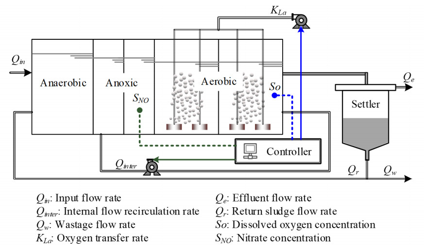
The objective of BWWTP is to diminish the quantity of organic matter, nitrogen, phosphorus, and suspended solids to render the wastewater clean. Figure 1 displays the BWWTP schematic view, including three compartments and one settler.

Robust multivariable tracking control for biological wastewater treatment process with external disturbances and uncertainties

Figure 1. Schematic view of BWWTP.

The first compartment serves as an anaerobic zone for the denitrification of returning sludge (external recycle) from the secondary settler. The second compartment offers an anaerobic environment for the denitrification of nitrite/nitrate recirculation from the preceding aerobic chamber. This compartment regulates the peristaltic pumps to control the intake, mixed liquor flow, and return sludge flow. The third compartment serves as an aerobic zone for the decomposition of organic waste into inorganic matter, using air pumps to provide oxygen. Furthermore, a dependable control system regulates effluent quality at the appropriate stations by managing aeration and sludge recycling flow rates.

The process of BWWTP is inherently complicated, nonlinear, and characterized by significant disruptions and uncertainty. The dynamic model of BWWTP may be articulated as follows[42]

$$ \begin{equation} \begin{cases} \dfrac{dS_{NO}(t)}{dt} = -\dfrac{1}{Y} \mu(t) X(t) + \{ S_{NO, in} - (1 + \omega(t)) S_{NO} \} D(t), \\ \dfrac{dS_O(t)}{dt} = -\dfrac{K_0}{Y} \mu(t) X(t) - D(t) (1 + \omega(t)) S_O(t) + K_L a(t) (S_{O, S} - S_O(t)) + S_{O, in} D(t), \\ \dfrac{dX(t)}{dt} = \mu(t) X(t) + D(t) (1 + \omega(t)) S_O(t) - r X_r(t) D(t), \\ \dfrac{dX_r(t)}{dt} = D(t) (1 + \omega(t)) X(t) - D(t) (\zeta(t) + \omega(t)) X_r(t). \end{cases} \end{equation} $$

where $$ S_{NO}(t) $$, $$ S_O(t) $$, $$ X(t) $$, and $$ X_r(t) $$ are the state variables representing the nitrate, the dissolved oxygen, the biomass, and the recycled biomass concentrations, $$ \omega(t) $$ and $$ \zeta(t) $$ represent the ratio of recycled flow to influent flow and the ratio of waste flow to influent flow, $$ S_{NO, in} $$ and $$ S_{O, in} $$ are the nitrate and dissolved oxygen concentrations in the feed stream. The dynamics of cell mass production are defined in terms of the specific growth rate $$ \mu $$ and the cell mass $$ Y $$, $$ K_0 $$ is a constant, $$ S_{O, s} $$ is the maximum dissolved oxygen concentration and $$ K_{L}a(t) $$ denotes the oxygen transfer rate, $$ D(t) $$ is the dilution rate, which is the linear correlation with $$ Q_{inter}(t) $$. Based on Equation 1, a simplified model denoted by control input and output is given as

$$ \begin{equation} \begin{cases} \dot{\mathbf{x}}(t) = \mathbf{f}(\mathbf{x}(t), \mathbf{u}(t)) + \mathbf{d}(t), \\ \mathbf{y}(t) = \mathbf{x}(t). \end{cases} \end{equation} $$

where $$ \mathbf{f}(\cdot) $$ is the unknown nonlinear function and sufficiently smooth, $$ \mathbf{x}(t)\in \mathbb{R}^{m \times 1} $$ denotes the state vector, $$ m $$ is the state's number, $$ \dot{\mathbf{x}}(t)\in \mathbb{R}^{m \times 1} $$ represents the deviation of $$ \mathbf{x}(t) $$, which is calculated by the subtraction between the intervals of $$ \mathbf{x}(t) $$. $$ \mathbf{u}(t)\in \mathbb{R}^{m \times 1} $$ denotes the control input vector, $$ \mathbf{d}(t)\in \mathbb{R}^{m \times 1} $$ represent the vectors of external disturbances, respectively, $$ \mathbf{y}(t)\in \mathbb{R}^{m \times 1} $$ denotes the vector of control output. In BWWTP, the state and control input are defined as $$ \mathbf{x}(t) = [S_{NO}(t), S_O(t)]^\mathrm{T} $$ and $$ \mathbf{u}(t) = [Q_{inter}(t), K_{L}a(t)]^\mathrm{T} $$. Different from the affine nonlinear systems[20], [22], and [36], the nonaffine nonlinear system given as Equation 2 is available for BWWTP because the control input does not appear linearly.

2.2. External disturbances and uncertainties

External disturbances are widespread in the BWWTP, such as the changes in influent flow rate, the unknown noise of sensors, and so on [7]. They are regarded as the combinations of unknown external disturbances. Correspondingly, the unknown $$ \mathbf{d}(t) $$ is continuous for all $$ t \geq 0 $$, as well as satisfies the conditions $$ |\mathbf{d}(t)| < \varepsilon_d $$, $$ \varepsilon_d $$ is a positive constant. The uncertainties include the nitrate production rate, the decreased nitrification, the settling velocity in the secondary clarifier, etc.[8]. The dynamic of uncertainties is related to the state and the external disturbances.

Notably, the external disturbances and uncertainties also exist not only in BWWTP simultaneously but also in other similar fields that have bioprocesses, chemical processes, biochemical processes, etc. The challenge of the control for these fields is to reject the disturbances and further ensure acceptable performance.

3. PROCESS DESCRIPTION

The scheme of RMTC, the direct controller, the approximate controller, the adaptive strategy, and the discussion of stability are presented in the subsequent sections.

3.1. Scheme of RMTC

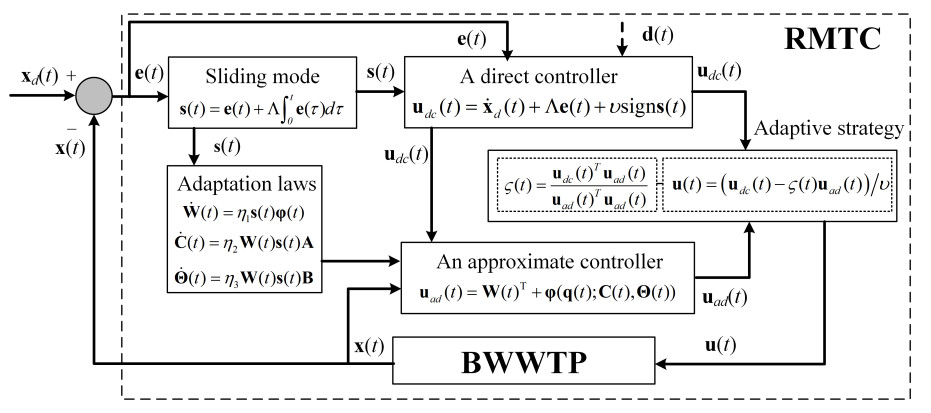
As shown in Figure 2, the proposed RMTC, including a direct controller and an approximate controller, as well as the adaptive technique, is recommended to achieve the strong performance of BWWTP.

Robust multivariable tracking control for biological wastewater treatment process with external disturbances and uncertainties

Figure 2. Robust multivariable tracking control for BWWTP.

In this RMTC, a direct controller and an approximate controller are designed with different control targets separately. The direct controller is designed to mitigate external disturbances caused by varying environmental conditions and inflow loads. The approximate controller is developed to compensate for the uncertainties by using a SOFNN. Then, by alleviating the influence of external disturbances and approximation errors, an adaptive strategy for balancing the performance of direct and approximate controllers is introduced to optimize the control gain and adjust the parameters of RMTC to hold the steady-state control performance under different operational conditions.

For RMTC, the tracking error $$ \mathbf{e}(t) $$ is given as

$$ \begin{equation} \mathbf{e}(t) = \mathbf{x}_d(t) - \mathbf{x}(t) \end{equation} $$

where $$ \mathbf{x}_d(t) $$ denotes the vector of bounded reference. The target of RMTC is to obtain a desired control law for Equation 3, and $$ \mathbf{e}(t) $$ can converge to zero. Assume that $$ \partial \mathbf{f}(\cdot)/\partial \mathbf{u}(t) $$ is invertible and satisfy $$ \|\partial \mathbf{f}(\cdot)/\partial \mathbf{u}(t)\| > f_0 $$, where $$ f_0 $$ is a positive constant. Nonaffine nonlinear functions in Equation 2 are performed using Taylor series expansion in the neighborhood of the ideal control laws $$ \mathbf{u}(t) $$[34]. It is given by

$$ \begin{equation} \begin{aligned} \mathbf{f}(\mathbf{x}(t), \mathbf{u}(t)) &= \mathbf{f}\big(\mathbf{x}(t), \mathbf{u}(t)^*\big) + \frac{\partial \mathbf{f}}{\partial \mathbf{u}(t)} \big( \mathbf{u}(t) - \mathbf{u}(t)^* \big) \\ &\quad + \Delta\big( \mathbf{x}(t), \mathbf{u}(t), \mathbf{u}(t)^* \big). \end{aligned} \end{equation} $$

To simplify Equation 4, there is

$$ \begin{equation} \mathbf{f}\big(\mathbf{x}(t), \mathbf{u}(t)\big) = \mathbf{g}(t) + \mathbf{G}\big(\mathbf{x}(t)\big) \mathbf{u}(t) + \nu \Delta\big(\mathbf{x}(t), \mathbf{u}(t)\big) \end{equation} $$

where

$$ \begin{equation} \mathbf{g}(t) = \mathbf{f}\big(\mathbf{x}(t), \mathbf{u}(t)^*\big) - \frac{\partial \mathbf{f}}{\partial \mathbf{u}(t)} \mathbf{u}(t)^*, \end{equation} $$

$$ \begin{equation} \mathbf{G}\big(\mathbf{x}(t)\big) = \frac{\partial \mathbf{f}}{\partial \mathbf{u}(t)} = \begin{bmatrix} \frac{\partial f_1(t)}{\partial u_{n+1}(t)} & \cdots & \frac{\partial f_1(t)}{\partial u_{2n}(t)} \\ \vdots & \ddots & \vdots \\ \frac{\partial f_n(t)}{\partial u_{n+1}(t)} & \cdots & \frac{\partial f_n(t)}{\partial u_{2n}(t)} \end{bmatrix} = \begin{bmatrix} \mathbf{G}_{1, 1}\big(\mathbf{x}(t)\big) & \cdots & \mathbf{G}_{1, n}\big(\mathbf{x}(t)\big) \\ \vdots & \ddots & \vdots \\ \mathbf{G}_{n, 1}\big(\mathbf{x}(t)\big) & \cdots & \mathbf{G}_{n, n}\big(\mathbf{x}(t)\big) \end{bmatrix}, \end{equation} $$

and $$ \mathbf{g}(t) = [g_1(t), \ldots, g_n(t)]^\mathrm{T} $$, $$ \Delta(\mathbf{x}(t), \mathbf{u}(t)) $$ represents the high-order term of the expression, $$ v $$ is the control gain that is larger than $$ \varepsilon_d $$. Let $$ \mathbf{g}(t) \equiv \mathbf{f}(\mathbf{x}(t), \mathbf{u}(t)) - v\mathbf{u}(t) $$, and $$ \mathbf{u}(t) $$ can be defined as

$$ \begin{equation} \mathbf{u}(t) = \frac{1}{v} \big( \mathbf{u}_{dc}(t) - \varsigma(t)\mathbf{u}_{ad}(t) \big), \end{equation} $$

where $$ \mathbf{u}_{dc}(t) $$ is the control input to suppress the external disturbances, $$ \mathbf{u}_{ad}(t) $$ is the adaptive control input to address $$ \mathbf{f}(\mathbf{x}(t), \mathbf{u}(t)) $$ using the proposed SOFNN, and $$ \varsigma(t) $$ is the adaptive parameter. Substituting Equation 6 into Equation 5, it will be

$$ \begin{equation} \dot{\mathbf{x}}(t) = \mathbf{u}_{dc}(t) + \mathbf{d}(t) + \big[ \mathbf{g}(t) - \mathbf{u}_{ad}(t) \big], \end{equation} $$

where $$ \mathbf{g}(\cdot) $$ indicates the unknown smooth function that denotes the nonlinear dynamics of the state. If it always satisfies $$ \mathbf{u}_{ad}(t) = \mathbf{g}(t) $$, we will just consider the external disturbances.

Remark 1: In order to avoid the complicated derivations and extra designs for its nonaffine counterpart, the system of BWWTP is transformed into a normal affine nonlinear form. As a result, there is the remainder of Taylor expansion in this step, which may bring deviation for control of BWWTP. Therefore, the control law in this work is decomposed and further obtained with a direct controller and an approximate controller. An approximate control has another role that compensates for the remainder derived from the uncertainties.

Remark 2: The two expressions of $$ \mathbf{g}(t) $$ are based on rigorous deductions under ideal control laws $$ \mathbf{u}(t)^* $$ and the design requirements of actual control laws $$ \mathbf{u}(t) $$, respectively. The form of $$ \mathbf{g}(t) $$ defined based on $$ \mathbf{u}(t)^* $$ is a result of rigorous deductions. This form reflects the nonlinear dynamic characteristics of the system under theoretically optimal conditions. In actual control, it is necessary to design $$ \mathbf{u}(t) $$ to approximate $$ \mathbf{u}(t)^* $$. Therefore, the control gain $$ v $$ is introduced and $$ \mathbf{g}(t) $$ is defined by $$ \mathbf{u}(t) $$. This transformation is used to derive the actual control laws $$ \mathbf{u}(t) $$. Then, it achieves integration between the direct controller $$ \mathbf{u}_{dc}(t) $$ and the approximate controller $$ \mathbf{u}_{ad}(t) $$, allowing the actual control input $$ \mathbf{u}(t) $$ to approach $$ \mathbf{u}(t)^* $$ through adaptive strategy adjustment, finally realizing target tracking.

3.2. Direct controller

The SMC serves as a proficient instrument for nonlinear systems, which is insensitive to external disturbances in the whole control period[23]. Consequently, the direct controller is designed with SMC. The control law of direct controller is given as:

$$ \begin{equation} \mathbf{u}_{dc}(t) = \dot{\mathbf{x}}_d(t) + \boldsymbol{\Lambda} \mathbf{e}(t) + \upsilon \, \text{sign}\big( \mathbf{s}(t) \big), \end{equation} $$

where $$ \dot{\mathbf{x}}_d(t) $$ is the first derivation of $$ \mathbf{x}_d(t) $$, $$ \dot{\mathbf{x}}_d(t) = \mathbf{x}_d(t+1) - \mathbf{x}_d(t) $$, $$ \boldsymbol{\Lambda} \in \mathbb{R}^{n \times n} $$ is the positive-definite diagonal matrix, $$ \mathbf{s}(t) $$ is defined as the instantaneous measure of performance that is described with a time-varying sliding surface by

$$ \begin{equation} \mathbf{s}(t) = \mathbf{e}(t) + \boldsymbol{\Lambda} \int_0^t \mathbf{e}(\tau) d\tau, \end{equation} $$

where $$ \tau $$ denotes the instantaneous measure time. The task of the direct controller is to achieve the desired $$ \mathbf{u}_{dc}(t) $$ such that all control output is uniformly bounded for all $$ t \geq 0 $$, and $$ \mathbf{e}(t) $$ can converge to zero. The derivative of $$ \mathbf{s}(t) $$ is given as

$$ \begin{equation} \dot{\mathbf{s}}(t) = -\boldsymbol{\varepsilon}(t) - \mathbf{d}(t) - \upsilon \, \text{sign}\big( \mathbf{s}(t) \big), \end{equation} $$

where $$ \boldsymbol{\varepsilon}(t) = \mathbf{g}(t) $$, $$ \text{sign}(\cdot) $$ is the sign function, if $$ \mathbf{s}(t) $$ is positive/negative, it outputs $$ \pm 1 $$; if $$ \mathbf{s}(t) $$ is zero, it outputs $$ 0 $$.

According to the theory of SMC, a Lyapunov candidate function is selected as

$$ \begin{equation} V_1(t) = \frac{1}{2} \mathbf{s}(t)^\mathrm{T} \mathbf{s}(t). \end{equation} $$

Differentiating Equation 13 with respect to time $$ t $$, it will be

$$ \begin{equation} \begin{aligned} \dot{V}_1(t) &= \mathbf{s}(t)^\mathrm{T} \big( -\boldsymbol{\varepsilon}(t) - \mathbf{d}(t) - \upsilon \, \text{sign}\big( \mathbf{s}(t) \big) \big) \\ &\leq - \big( \upsilon - \|\mathbf{d}(t)\| - \|\boldsymbol{\varepsilon}(t)\| \big) \|\mathbf{s}(t)\|. \end{aligned} \end{equation} $$

When the system maintains stability according to the Lyapunov theorem, there is $$ \dot{V}_1(t) < 0 $$. So, the conditions associated with $$ \lim\limits_{t \to \infty} \|\boldsymbol{\varepsilon}(t)\| = 0 $$ and $$ \|\mathbf{d}_\mathrm{ext}(t)\| < \upsilon $$ should be satisfied. However, the sliding-mode function and the desired $$ \mathbf{u}_{ad}(t) $$ cannot be accurately determined. Furthermore, a substantial control gain $$ \upsilon $$ is often necessary to provide rapid reaction and precise control. Consequently, it will result in superfluous deviations from the switching surface, leading to the inevitable chattering phenomenon. To deal with this issue, FNN is employed to assess the system's dynamics and further conquer the chattering phenomenon. Compared to NN, FNN is equipped with fuzzy rules that can achieve fuzzy "blending" of dynamics with membership functions by imposing stricter limits on the range and accuracy of input information. Thus, it has strong robustness to handle the dynamics of the system characterized by uncertain information and disturbances.

3.3. Approximate controller

It can be seen from Equation 13 that it is necessary for the controller to obtain an ideal $$ \mathbf{g}(t) $$ to achieve $$ \lim\limits_{t \to \infty} \|\boldsymbol{\varepsilon}(t)\| = 0 $$. Based on the universal approximation theorem, an approximate controller is designed with a one-step-ahead state predictor to estimate the uncertain dynamics of BWWTP

$$ \begin{equation} \mathbf{u}_{ad}(t) = \hat{\mathbf{g}}(t), \end{equation} $$

where $$ \hat{\mathbf{g}}(t) $$ is to estimate $$ \mathbf{u}_{ad}(t) $$ by using FNN which is equipped with $$ o $$-$$ h $$-$$ h $$-$$ k $$ topology, and $$ o $$ is the input variables number, $$ h $$ is the fuzzy rules number, $$ k $$ is the number of output variables. The input and output vectors of FNN are $$ \mathbf{q}(t) = [q_1(t), q_2(t), \ldots, q_o(t)]^\mathrm{T} $$ and $$ \hat{\mathbf{g}}(t) = [\hat{g}_1(t), \hat{g}_2(t), \ldots, \hat{g}_k(t)] $$. The input vector $$ \mathbf{q}(t) $$ are $$ \{ \mathbf{x}(t), \mathbf{u}_{dc}(t) \} $$, $$ \mathbf{d}_\mathrm{int}(t) $$, $$ \mathbf{u}^*(t) (:=\mathbf{u}_{dc}(t)) $$ according to Equation 12. The dynamic of $$ \mathbf{d}_\mathrm{int}(t) $$ is obtained when $$ \mathbf{u}^*(t) $$ is set to zero according to Equation 4.

Then,

$$ \begin{equation} \mathbf{g}(t) = \hat{\mathbf{g}}(t) + \boldsymbol{\varepsilon}(t) = \mathbf{W}(t)^\mathrm{T} \boldsymbol{\varphi}\big( \mathbf{q}(t); \mathbf{C}(t), \boldsymbol{\Theta}(t) \big) + \boldsymbol{\varepsilon}(t), \end{equation} $$

where $$ \mathbf{W}(t) = [\mathbf{w}_1(t), \mathbf{w}_2(t), \ldots, \mathbf{w}_k(t)]^\mathrm{T} $$ denotes a vector of unknown weight matrix.

$$ \boldsymbol{\varphi}(\cdot) = [\varphi_1(\cdot), \varphi_2(\cdot), \ldots, \varphi_h(\cdot)]^\mathrm{T} $$ is a bounded continuous regressor which is defined as

$$ \begin{equation} \varphi_l(t) = \exp\big( - (\mathbf{q}(t) - \mathbf{c}_l(t))^\mathrm{T} \boldsymbol{\Sigma}_l^{-2}(t) (\mathbf{q}(t) - \mathbf{c}_l(t)) \big), \end{equation} $$

where $$ \mathbf{C}(t) = [\mathbf{c}_1(t), \mathbf{c}_2(t), \ldots, \mathbf{c}_h(t)] $$ and $$ \boldsymbol{\Theta}(t) = [\boldsymbol{\sigma}_1(t), \boldsymbol{\sigma}_2(t), \ldots, \boldsymbol{\sigma}_h(t)] $$, $$ \mathbf{c}_l(t) = [c_{1l}(t), c_{2l}(t), \ldots, c_{ol}(t)]^\mathrm{T} $$ and $$ \boldsymbol{\sigma}_l(t) = [\sigma_{1l}(t), \sigma_{2l}(t), \ldots, \sigma_{ol}(t)]^\mathrm{T} $$ ($$ l = 1, 2, \ldots, h $$) are the vectors of centers and widths, $$ \varphi_l(\cdot) $$ is the activation function of the $$ l $$th fuzzy rule in normalized layer, $$ \boldsymbol{\Sigma}_l(t) = \mathrm{diag}(\sigma_{1l}(t), \sigma_{2l}(t), \ldots, \sigma_{ol}(t)) $$. All these parameters are bounded over the compact set $$ \Gamma_{\mathbf{q}} \in \mathbb{R}^o $$ and the width of a fuzzy set is positive, and $$ \boldsymbol{\varepsilon}(t) $$ satisfies $$ \|\boldsymbol{\varepsilon}(t)\| \leq \varepsilon_0(t) $$, $$ \varepsilon_0(t) $$ is an unknown bound parameter. Considering the characteristics of the data-driven model using a neural network, the predictor using FNN can uniformly approximate the continuous function $$ \mathbf{g}(t) $$ with a proper number of fuzzy rules by

$$ \begin{equation} \mathbf{g}(t) = \mathbf{W}^*(t)^\mathrm{T} \boldsymbol{\varphi}\big( \mathbf{q}(t); \mathbf{C}^*(t), \boldsymbol{\Theta}^*(t) \big) + \boldsymbol{\varepsilon}^*(t), \end{equation} $$

where $$ \mathbf{W}^*(t) $$, $$ \mathbf{C}^*(t) $$, and $$ \boldsymbol{\Theta}^*(t) $$ are the ideal weight, centers, and widths matrix of SOFNN, $$ \boldsymbol{\varepsilon}^*(t) $$ is the approximation errors for the case $$ \mathbf{W}(t) = \mathbf{W}^*(t) $$, $$ \mathbf{C}(t) = \mathbf{C}^*(t) $$ and $$ \boldsymbol{\Theta}(t) = \boldsymbol{\Theta}^*(t) $$. The optimal parameters of SOFNN over the compact set $$ \Gamma_{\mathbf{q}} $$ can be described as

$$ \begin{equation} \big\{ \mathbf{W}^*(t), \mathbf{C}^*(t), \boldsymbol{\Theta}^*(t) \big\} = \arg \min \left[ \max\limits_{\mathbf{q} \in \Gamma_{\mathbf{q}}} \big\| \hat{\mathbf{g}}(t) - \mathbf{g}(t) \big\| \right]. \end{equation} $$

The structure of NN or FNN in previous studies associated with the design of the controller is always predefined with prior knowledge or trials and errors. Besides, it also maintains constant except for the parameters of the controller updated by adaptive laws. This fact may lead to inaccurate approximation for BWWTP with obvious dynamics and serious disturbances due to mismatched fuzzy rules.

As to FNN, it needs enough fuzzy rules to cover the dynamics of systems, which also brings the risk of structural redundancy. Therefore, the choice of fuzzy rules without prior knowledge is difficult. To deal with the challenge, there are two criteria, i.e., its empirical error and structural complexity associated with its performance that can be used for optimizing the FNN's structure. The empirical error is

$$ \begin{equation} \omega_1(t_g) = \boldsymbol{\varepsilon}(t)^\mathrm{T} \boldsymbol{\varepsilon}(t), \end{equation} $$

where $$ t_g $$ represents the number of sampling intervals. Correspondingly, the structural complexity of FNN is defined as:

$$ \begin{equation} \omega_2(t_g) = \frac{ \sqrt{ o h(t_g) \log n } - 2 \log h(t_g) }{ \sqrt{n} }, \end{equation} $$

where $$ n $$ is the discrete-time performed during the control process, and $$ h(t_g) $$ is the fuzzy rules number at $$ t_g $$. The construction of the structural complexity Equation 21 integrates the local Rademacher complexity with the $$ L_1 $$-metric capacity and the Structural Risk Minimization (SRM) principle[36], which is employed to minimize the empirical risk over the $$ n $$th hypothesis space. Based on the $$ L_1 $$-metric capacity, the main term $$ \sqrt{ o h(t_g) \log n } $$ is used to accurately characterize the contribution of the fuzzy rules number $$ h(t_g) $$ and the input dimension $$ o $$ to the structural complexity. Among them, $$ \log n $$ is based on the sample size dependent boundary of local Rademacher complexity, reflecting the impact of the sample scale on the upper bound of complexity. Besides, the penalty term $$ -2 \log h(t_g) $$ is inspired by the information theoretic criteria. It suppresses the rule redundancy in the form of a negative logarithm. The normalization factor $$ 1 / \sqrt{n} $$ balances the complexity term with the convergence rate of the generalization error, ensuring that the structural complexity is controllable as the sample size increases.

To achieve accurate approximation and compact structure, it is critical to find the optimal $$ h(t_g) $$ by

$$ \begin{equation} h(t_g) = \arg \min\limits_{\mathbf{q} \in \Gamma_{\mathbf{q}}} \big( \omega_1(t_g), \omega_2(t_g) \big). \end{equation} $$

Different from the parameters shown in Equation 19, the update of the fuzzy rules number is discrete. It is challenging to conduct when the output should be smooth and stable. To remove this obstacle, a continuous function $$ \kappa(t_g) $$ is introduced to replace $$ h(t_g) $$ in $$ [t_g, t_g+1) $$. It satisfies the condition $$ \kappa(t_g) = h(t_g) $$. According to the structural risk evaluation[25], assuming that the object of optimization for $$ h(t_g) $$ is a linear regression function between $$ \omega_1(t_g) $$ and $$ \omega_2(t_g) $$, and $$ \omega_1(t_g) $$ remains constant with proper initialization of parameters in $$ [t_g, t_g+1) $$, the derivative of $$ \kappa(t_g) $$ to the error of approximation can be given as

$$ \begin{equation} \dot{\kappa}(t_g) = \sqrt{ o \log n / n \kappa(t_g) } / 2 - 2 / \sqrt{n} \kappa(t_g). \end{equation} $$

This derivative reflects the impact of fuzzy rules number on the FNN's performance. It can be employed to direct the update of fuzzy rules. Then, the SOFNN is built as:

(1) Adding Fuzzy Rule: When the derivative satisfies

$$ \begin{equation} \dot{\kappa}(t_g) < \gamma_1, \end{equation} $$

where $$ \gamma_1 $$ is a threshold value, a new fuzzy rule is inserted into FNN. The parameters of this rule will be set

$$ \begin{equation} \begin{split} \boldsymbol{c}_{new} = &\boldsymbol{q}(t), \boldsymbol{\sigma}_{new} = h^{-1} \sum\limits_{i=1}^h \boldsymbol{\sigma}_i(t), \mathbf{w}_{new} = \boldsymbol{\varepsilon}(t) \exp\bigl(\boldsymbol{q}(t), \boldsymbol{c}_{new}, \boldsymbol{\sigma}_{new}\bigr), \\ &\exp\bigl(\boldsymbol{q}(t), \boldsymbol{c}_{new}, \boldsymbol{\sigma}_{new}\bigr) = \sum\limits_{i=1}^h \bigl\lVert \boldsymbol{q}(t) - \boldsymbol{c}_{new} \bigr\rVert^2 / 2 \bigl\lVert \boldsymbol{\sigma}_{new} \bigr\rVert^2, \end{split} \end{equation} $$

where $$ \boldsymbol{c}_{new} $$, $$ \boldsymbol{\sigma}_{new} $$ and $$ \mathbf{w}_{new} $$ represent the center, width and weight of the new rule.

(2) Pruning Fuzzy Rule: If the derivative meets

$$ \begin{equation} \dot{\kappa}(t_g) \geq \gamma_2, \varphi_j(t) = \min\limits_{l = 1, \dots, j, \dots, h} \varphi_l(t), \end{equation} $$

where $$ \gamma_2 > 0 $$ is a predefined threshold. The $$ j $$th rule with the minimum $$ \varphi_j(t) $$ will be pruned. The parameters of the $$ i $$th rule (the $$ i $$th rule is nearest to the $$ j $$th rule with the smallest Euclidean distance) are updated as

$$ \begin{equation} \begin{split} \mathbf{c}_i(t + 1) &= \mathbf{c}_i(t), \boldsymbol{\sigma}_i(t + 1) = \boldsymbol{\sigma}_i(t), \\ \mathbf{w}_i(t + 1) &= \mathbf{I} + \frac{\mathbf{w}_j(t) \exp(\mathbf{q}(t), \mathbf{c}_j(t), \boldsymbol{\sigma}_j(t))}{\|\mathbf{w}_i(t) \exp(\mathbf{q}(t), \mathbf{c}_j(t), \boldsymbol{\sigma}_j(t))\|}, \end{split} \end{equation} $$

where $$ \mathbf{c}_i(t + 1) $$ and $$ \boldsymbol{\sigma}_i(t + 1) $$ are the centers and the width of the $$ i $$th rule after the structure has been adjusted, $$ \mathbf{c}_i(t) $$ and $$ \boldsymbol{\sigma}_i(t) $$ are the centers and the width of the $$ i $$th rule before the structure has been adjusted, $$ \mathbf{w}_i(t + 1) $$ and $$ \mathbf{w}_i(t) $$ are the weights of the $$ i $$th rule after and before the structure had been adjusted, and all elements of vector $$ \mathbf{I} $$ is 1.

Remark 3: The criterion[25] is introduced to evaluate the effectiveness of fuzzy rules. It is used to optimize the number of fuzzy rules by balancing the approximation error and structure complexity. With a compact structure, FNN's generality will be enhanced during approximation for BWWTP, which can strengthen the robustness of RMTC.

3.4. Adaptive strategy

To accomplish the optimization of parameters in Equation 19 an adaptive strategy is developed to obtain adaptation laws of parameters $$ \mathbf{W}(t) $$, $$ \mathbf{C}(t) $$, $$ \boldsymbol{\Theta}(t) $$ by using the projection modification. Firstly, we consider the Lyapunov candidate function as

$$ \begin{equation} \begin{split} V_2(t) &= \frac{1}{2}\mathbf{s}(t)^\mathrm{T}\mathbf{s}(t) + \frac{1}{2}\mathbf{e}(t)^\mathrm{T}\mathbf{e}(t) \\ &\quad + \frac{1}{2\eta_a}\tilde{\mathbf{W}}(t)^\mathrm{T}\tilde{\mathbf{W}}(t) + \frac{1}{2\eta_b}\tilde{\mathbf{C}}(t)^\mathrm{T}\tilde{\mathbf{C}}(t) \\ &\quad + \frac{1}{2\eta_c}\tilde{\boldsymbol{\Theta}}(t)^\mathrm{T}\tilde{\boldsymbol{\Theta}}(t), \end{split} \end{equation} $$

where $$ \tilde{\mathbf{W}}(t), \tilde{\mathbf{C}}(t) $$ and $$ \tilde{\boldsymbol{\Theta}}(t) $$ are estimation error of parameters, and $$ \tilde{\mathbf{W}}(t)=\mathbf{W}(t)-\mathbf{W}^*(t) $$, $$ \tilde{\mathbf{C}}(t)=\mathbf{C}(t)-\mathbf{C}^*(t) $$, $$ \tilde{\boldsymbol{\Theta}}(t)=\boldsymbol{\Theta}(t)-\boldsymbol{\Theta}^*(t) $$. $$ \eta_a $$, $$ \eta_b $$ and $$ \eta_c $$ are the constants.

The time derivative of \(V_2(t) \) is

$$ \begin{equation} \begin{split} \dot{V}_2(t) &= \mathbf{s}(t)^\mathrm{T} \dot{\mathbf{s}}(t) + \mathbf{e}(t)^\mathrm{T} \dot{\mathbf{e}}(t) + \frac{1}{\eta_a} \tilde{\mathbf{W}}(t)^\mathrm{T} \dot{\tilde{\mathbf{W}}}(t) \\ &\quad + \frac{1}{\eta_b} \tilde{\mathbf{C}}(t)^\mathrm{T} \dot{\tilde{\mathbf{C}}}(t) + \frac{1}{\eta_c} \tilde{\boldsymbol{\Theta}}(t)^\mathrm{T} \dot{\tilde{\boldsymbol{\Theta}}}(t), \end{split} \end{equation} $$

Combining with Equation 9, Equation 10, and Equation 14, it has

$$ \begin{equation} \begin{split} \dot{V}_2(t) &= -\mathbf{s}(t)^\mathrm{T} \big( \boldsymbol{\varepsilon}(t) + \mathbf{d}(t) + v \mathrm{sign}(\mathbf{s}(t)) \big) - \mathbf{e}(t)^\mathrm{T} \boldsymbol{\Lambda} \mathbf{e}(t) \\ &\quad - \mathbf{e}(t)^\mathrm{T} \big( \dot{\mathbf{x}}_d(t) + v \mathrm{sign}(\mathbf{s}(t)) + \mathbf{d}(t) \big) \\ &\quad + \frac{1}{\eta_a} \tilde{\mathbf{W}}(t)^\mathrm{T} \dot{\tilde{\mathbf{W}}}(t) + \frac{1}{\eta_b} \tilde{\mathbf{C}}(t)^\mathrm{T} \dot{\tilde{\mathbf{C}}}(t) + \frac{1}{\eta_c} \tilde{\boldsymbol{\Theta}}(t)^\mathrm{T} \dot{\tilde{\boldsymbol{\Theta}}}(t), \end{split} \end{equation} $$

Based on Equation 16 and Equation 18, the estimated error $$ \boldsymbol{\varepsilon}(t) $$ is

$$ \begin{equation} \begin{split} \boldsymbol{\varepsilon}(t) &= \tilde{\mathbf{W}}(t)^\mathrm{T} \boldsymbol{\varphi}(t) + \tilde{\mathbf{C}}(t)^\mathrm{T} \mathbf{Q}_1 \mathbf{W}(t) \\ &\quad + \tilde{\boldsymbol{\Theta}}(t)^\mathrm{T} \mathbf{Q}_2 \mathbf{W}(t) + \boldsymbol{\Delta}(t), \end{split} \end{equation} $$

where

$$ \begin{equation} \mathbf{Q}_1 = \left[ \frac{\partial \varphi_1(t)}{\partial \mathbf{C}(t)}, \dots, \frac{\partial \varphi_o(t)}{\partial \mathbf{C}(t)} \right], \quad \mathbf{Q}_2 = \left[ \frac{\partial \varphi_1(t)}{\partial \boldsymbol{\Theta}(t)}, \dots, \frac{\partial \varphi_o(t)}{\partial \boldsymbol{\Theta}(t)} \right], \end{equation} $$

and $$ \boldsymbol{\Delta}(t) $$ is the vector of higher-order terms of the Taylor series and is defined as

$$ \begin{equation} \boldsymbol{\Delta}(t) = \mathbf{W}(t)^\mathrm{T} \tilde{\boldsymbol{\varphi}}(t) + \tilde{\mathbf{W}}(t)^\mathrm{T} \tilde{\boldsymbol{\varphi}}(t) + \boldsymbol{\varepsilon}^*(t). \end{equation} $$

Substituting Equation 31 into Equation 30, Equation 30 can be rewritten as

$$ \begin{equation} \begin{split} \dot{V}_2(t) &= -\mathbf{s}(t)^\mathrm{T} \big( \mathbf{d}(t) + \upsilon \, \text{sign}(\mathbf{s}(t)) + \boldsymbol{\Delta}(t) \big) \\ &\quad - \mathbf{e}(t)^\mathrm{T} \big( \dot{\mathbf{x}}_d(t) + \mathbf{d}(t) + \upsilon \, \text{sign}(\mathbf{s}(t)) \big) - \mathbf{e}(t)^\mathrm{T} \boldsymbol{\Lambda} \mathbf{e}(t) \\ &\quad + \tilde{\mathbf{W}}(t)^\mathrm{T} \left( \frac{1}{\eta_a} \dot{\tilde{\mathbf{W}}}(t) - \boldsymbol{\varphi}(t) \mathbf{s}(t) \right) \\ &\quad + \tilde{\mathbf{C}}(t)^\mathrm{T} \left( \frac{1}{\eta_b} \dot{\tilde{\mathbf{C}}}(t) - \mathbf{W}(t) \mathbf{s}(t) \mathbf{Q}_1(t) \right) \\ &\quad + \tilde{\boldsymbol{\Theta}}(t)^\mathrm{T} \left( \frac{1}{\eta_c} \dot{\tilde{\boldsymbol{\Theta}}}(t) - \mathbf{W}(t) \mathbf{s}(t) \mathbf{Q}_2(t) \right). \end{split} \end{equation} $$

The adaptation laws of parameters are thus selected as

$$ \begin{equation} \dot{\tilde{\mathbf{W}}}(t) = \eta_a \boldsymbol{\varphi}(t) \mathbf{s}(t), \end{equation} $$

$$ \begin{equation} \dot{\tilde{\mathbf{C}}}(t) = \eta_b \mathbf{W}(t) \mathbf{s}(t) \mathbf{Q}_1(t), \end{equation} $$

$$ \begin{equation} \dot{\tilde{\boldsymbol{\Theta}}}(t) = \eta_c \mathbf{W}(t) \mathbf{s}(t) \mathbf{Q}_2(t). \end{equation} $$

Taking Equation 35, Equation 36, and Equation 37 into Equation 34 yields

$$ \begin{equation} \begin{split} \dot{V}_2(t) &= -\mathbf{s}(t)^\mathrm{T} \big( \mathbf{d}(t) + \upsilon \, \text{sign}(\mathbf{s}(t)) + \boldsymbol{\Delta}(t) \big) \\ &\quad - \mathbf{e}(t)^\mathrm{T} \big( \dot{\mathbf{x}}_d(t) + \mathbf{d}(t) + \upsilon \, \text{sign}(\mathbf{s}(t)) \big) - \mathbf{e}(t)^\mathrm{T} \boldsymbol{\Lambda} \mathbf{e}(t) \\ &\leq -\mathbf{s}(t)^\mathrm{T} \big( \boldsymbol{\Delta}(t) + \mathbf{d}(t) + \upsilon \, \text{sign}(\mathbf{s}(t)) \big) \\ &\quad - \mathbf{e}(t)^\mathrm{T} \big( \dot{\mathbf{x}}_d(t) + \mathbf{d}(t) + \upsilon \, \text{sign}(\mathbf{s}(t)) \big). \end{split} \end{equation} $$

Applying Equation 11, if it satisfies that \(\upsilon > \|\dot{\mathbf{x}}_d(t)\|\) and \(\upsilon > \|\boldsymbol{\Delta}(t)\|\), it has

$$ \begin{equation} \begin{split} \dot{V}_2(t) &\leq -\mathbf{s}(t)^\mathrm{T} \big( \boldsymbol{\Delta}(t) + \mathbf{d}(t) + \upsilon \, \text{sign}(\mathbf{s}(t)) \big) \\ &\quad - \mathbf{e}(t)^\mathrm{T} \big( \dot{\mathbf{x}}_d(t) + \mathbf{d}(t) + \upsilon \, \text{sign}(\mathbf{e}(t)) \big) \\ &\leq -\mathbf{s}(t)^\mathrm{T} \big( \upsilon \, \text{sign}(\mathbf{s}(t)) \big) - \mathbf{e}(t)^\mathrm{T} \big( \upsilon \, \text{sign}(\mathbf{s}(t)) \big) \\ &\leq 0. \end{split} \end{equation} $$

Based on Equation 39, $$ \boldsymbol{\Delta}(t) $$ is the remainder term of approximation and is generated from the estimation of uncertain dynamics. Therefore, the selection of control gain $$ v $$ should be considered to take the external disturbances and uncertainties into account. Once the control gain $$ v $$ is enough large, there will be $$ \dot{V}_2(t) < 0 $$. Then, $$ \mathbf{e}(t) $$ can converge to zero. However, the chattering phenomenon may arise. Therefore, the adaptive parameter $$ \varsigma(t) $$ is to regulate the direct controller and the approximate controller. Then, an optimization technique is designed to adjust the adaptive parameter $$ \varsigma(t) $$

$$ \begin{equation} \mathbf{J}(t) = v \mathbf{u}(t)^\mathrm{T} \mathbf{u}(t) + (1 - v) \mathbf{e}(t)^\mathrm{T} \mathbf{e}(t), \end{equation} $$

where $$ v $$ ($$ 0 < v < 1 $$) is a weighting factor used to balance the control input term $$ \mathbf{u}(t)^\mathrm{T} \mathbf{u}(t) $$ and the tracking error term $$ \mathbf{e}(t)^\mathrm{T} \mathbf{e}(t) $$ in the objective function $$ \mathbf{J}(t) $$. When $$ v $$ is large, the objective function emphasizes suppressing fluctuations in the control input. This can reduce the chattering phenomenon that may be caused by SMC, making the control action smoother. When $$ v $$ is small, the objective function emphasizes reducing the tracking error. This can improve the system's tracking accuracy of the reference trajectory.

A feasible point $$ \varsigma^*(t) $$ for the optimization problem in Equation 40 is said to be the optimal solution if and only if there exists no other feasible point $$ \varsigma(t) $$

$$ \begin{equation} \mathbf{J}_i(\varsigma^*(t)) \leq \mathbf{J}_i(\varsigma(t)), \end{equation} $$

where \(i = 1, 2, \dots, n\). \(\varsigma^*(t) = \arg\min_{\varsigma^*(t) \in \Omega_f} \mathbf{J}(t)\) the optimal solution \(\varsigma^*(t)\) is over the compact set \(\Omega_f \in \Re\). The gradient algorithm is used to deal with this optimization problem. The derivative of \(\mathbf{J}(t)\) is given as

$$ \begin{equation} \frac{\partial \mathbf{J}(t)}{\partial \varsigma(t)} = 2v \mathbf{u}(t)^\mathrm{T} \frac{\partial \mathbf{u}(t)}{\partial \varsigma(t)} + 2(1 - v) \mathbf{e}(t)^\mathrm{T} \frac{\partial \mathbf{e}(t)}{\partial \varsigma(t)}. \end{equation} $$

From Equation 8, it will be \(\frac{\partial \mathbf{u}(t)}{\partial \varsigma(t)} = [\lambda \frac{\partial \mathbf{e}(t)}{\partial \varsigma(t)} - \mathbf{u}_{ad}(t)] / v\). Equation 41 can be rewritten as

$$ \begin{equation} \begin{split} \frac{\partial \mathbf{J}(t)}{\partial \varsigma(t)} &= \frac{2v}{\upsilon} \left[ \lambda \mathbf{u}(t) + \frac{(1 - v)\upsilon}{v} \mathbf{e}(t) \right]^\mathrm{T} \frac{\partial \mathbf{e}(t)}{\partial \varsigma(t)} \\ &\quad - \frac{2v}{\upsilon} \mathbf{u}(t)^\mathrm{T} \mathbf{u}_{ad}(t), \end{split} \end{equation} $$

The minimization of $$ \mathbf{J}(t) $$ is regarded as $$ \frac{\partial \mathbf{J}(t)}{\partial \varsigma(t)} = 0 $$. Equation 43 will be

$$ \begin{equation} \left[ \lambda^\mathrm{T} \mathbf{u}(t) + \frac{(1 - v)\upsilon}{v} \mathbf{e}(t) \right]^\mathrm{T} \frac{\partial \mathbf{e}(t)}{\partial \varsigma(t)} = \mathbf{u}(t)^\mathrm{T} \mathbf{u}_{ad}(t), \end{equation} $$

where

$$ \begin{equation} \mathbf{u}(t)^\mathrm{T} \mathbf{u}_{ad}(t) = \frac{1}{\upsilon} \big( \mathbf{u}_{dc}(t)^\mathrm{T} \mathbf{u}_{ad}(t) - \varsigma(t) \mathbf{u}_{ad}(t)^\mathrm{T} \mathbf{u}_{ad}(t) \big). \end{equation} $$

Suppose that $$ \lim_{t \to 0} \frac{\partial \mathbf{e}(t)}{\partial \varsigma(t)} = 0 $$, and $$ \varsigma(t) $$ is calculated by

$$ \begin{equation} \varsigma(t) = \frac{\mathbf{u}_{dc}(t)^\mathrm{T} \mathbf{u}_{ad}(t)}{\mathbf{u}_{ad}(t)^\mathrm{T} \mathbf{u}_{ad}(t)}. \end{equation} $$

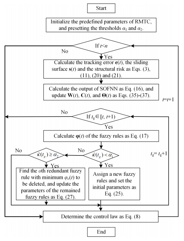
Figure 3 provides a summary of the primary RMTC steps.

Robust multivariable tracking control for biological wastewater treatment process with external disturbances and uncertainties

Figure 3. The flowchart of RMTC for BWWTP.

Remark 4: For this proposed RMTC, the high control accuracy with suitable approximation performance can be obtained by felicitously adjusting the adaptive parameter $$ \varsigma(t) $$. Based on this adaptive strategy, $$ \varsigma(t) $$ can balance the performance of the direct controller and the approximate controller, which maintain control accuracy and avoid serious chattering problems.

Remark 5: At the initial moment of the control system, the controller has not yet begun dynamic adjustment. At this moment, the tracking error $$ \mathbf{e}(t) $$ is determined by the initial state and has not yet established a connection with the adaptive parameter $$ \varsigma(t) $$. The sensitivity of the error to the parameter $$ \frac{\partial \mathbf{e}(t)}{\partial \varsigma(t)} $$ can be considered zero. Therefore, this characteristic at the initial moment is used as a simplification condition (i.e. $$ \lim_{t \to 0} \frac{\partial \mathbf{e}(t)}{\partial \varsigma(t)} = 0 $$) to simplify the deduction of the adaptive parameter $$ \varsigma(t) $$.

3.5. Stability analysis of RMTC

For the proposed RMTC, the stability of the control law is a critical topic that requires thorough examination, since it is essential for successful applications. The stability of the proposed controller is analyzed with sufficient conditions and parameters selection method.

Theorem. Consider the system given as Equation 2 with the control law as Equation 9. Suppose the number of fuzzy rules is \(h \), and the structure of SOFNN is adjusted according to Equation 25, Equation 26, Equation 27, and Equation 28, and its parameters are selected with Equation 36, Equation 37, and Equation 38. Besides, assume the following condition holds

$$ \begin{equation} \frac{1}{\kappa_1 - 1} < \gamma_1 < \frac{\kappa_2}{\kappa_2 - 1} < \gamma_2 < \frac{16}{o \log n}, \end{equation} $$

where \(\kappa_1 = e^{\frac{1}{2} \big(\sqrt{l(n)} + 1 - \sqrt{l(n)} \big) \sqrt{o \log n}}\), and \(\kappa_2 = e^{\frac{1}{2} \big(\sqrt{l(n)} - \sqrt{l(n) - 1} \big) \sqrt{o \log n}}\). Then, the stability of RMTC under disturbances can be guaranteed.

Proof. The candidate Lyapunov function is considered as follows

$$ \begin{equation} V_3(t) = V_2(t) + \frac{1}{2} \Gamma_{1, h}(t) + \frac{1}{2} \Gamma_{2, h}(t), \end{equation} $$

where $$ \Gamma_{1, h}(t) $$ and $$ \Gamma_{2, h}(t) $$ are the empirical error and the structural complexity according to Equation 21 and Equation 22, respectively. Once the fuzzy rules are added or pruned, the estimation error $$ \tilde{\boldsymbol{\varepsilon}}(t) $$ will be

$$ \begin{equation} \tilde{\boldsymbol{\varepsilon}}(t) = \hat{\mathbf{g}}(\mathbf{q}(t); \bar{h}(t)), \end{equation} $$

where $$ \bar{h}(t) $$ is the number of fuzzy rules after its adding or pruning. Based on Equation 25 and Equation 28, whatever the fuzzy rule is added or deleted in $$ [t_g, t_g + 1] $$, the output of approximation maintains an equivalent that satisfies

$$ \begin{equation} \begin{split} \Gamma_{1, h}(t_g + 1) - \Gamma_{1, h}(t_g) &= \tilde{\boldsymbol{\varepsilon}}(t_g + 1)^\mathrm{T} \tilde{\boldsymbol{\varepsilon}}(t_g + 1) - \tilde{\boldsymbol{\varepsilon}}(t_g)^\mathrm{T} \tilde{\boldsymbol{\varepsilon}}(t_g) \\ &= 0. \end{split} \end{equation} $$

Correspondingly, during the phase of fuzzy rule addition, the variation of structural complexity is

$$ \begin{equation} \begin{split} \Gamma_{2, h}(t_g + 1) - \Gamma_{2, h}(t_g) &= \frac{\sqrt{h(t_g + 1) o \log n} - 2 \log \big( h(t_g) + 1 \big)}{\sqrt{n}} \\ &\quad - \frac{\sqrt{h(t_g) o \log n} - 2 \log h(t_g)}{\sqrt{n}}. \end{split} \end{equation} $$

With the condition of Equation 47, Equation 51 satisfies

$$ \begin{equation} \Gamma_{2, h}(t_g + 1) - \Gamma_{2, h}(t_g) \leq \frac{2}{\sqrt{n}} \left( \log \kappa_1 - \log \frac{\gamma_1 + 1}{\gamma_1} \right) < 0. \end{equation} $$

Besides, once a fuzzy rule is pruned, the variation of structural complexity will be

$$ \begin{equation} \Gamma_{2, h}(t_g + 1) - \Gamma_{2, h}(t_g) \leq \frac{2}{\sqrt{n}} \left( \log \frac{1}{\kappa_1} - \log \frac{\gamma_2 - 1}{\gamma_2} \right) < 0. \end{equation} $$

According to the agreement between $$ t_g $$ and $$ t $$, the variation of empirical error and structural complexity can be rewritten by

$$ \begin{equation} \begin{split} \Gamma_{1, \bar{h}}(t) - \Gamma_{1, h}(t) &= 0, \\ \Gamma_{2, \bar{h}}(t) - \Gamma_{2, h}(t) &< 0, \end{split} \end{equation} $$

where $$ \Gamma_{1, \bar{h}}(t) $$ and $$ \Gamma_{2, \bar{h}}(t) $$ is structural complexity after the structure of FNN changes.

Therefore, the difference of Lyapunov function $$ V_3(t) $$ at $$ t = 0 $$ to $$ t = n $$ is

$$ \begin{equation} \begin{split} V_3(n) - V_1(0) &= V_3(n) - V_2(n) + V_2(n) - V_1(0) \\ &= \Gamma_{1, \bar{h}}(t) - \Gamma_{1, h}(t) + \Gamma_{2, \bar{h}}(t) \\ &\quad - \Gamma_{2, h}(t) + V_2(n) - V_1(0). \end{split} \end{equation} $$

By substituting Equation 36, Equation 37, Equation 38, Equation 51 and Equation 54 into Equation 55, it will be

$$ \begin{equation} \begin{split} V_3(n) - V_1(0) &< V_2(n) - V_1(0) \\ &\leq -\mathbf{s}(t)^\mathrm{T} \big( \boldsymbol{\Delta}(t) + \mathbf{d}_\mathrm{ext}(t) + \upsilon \mathbf{I} \big) \\ &\quad - \mathbf{e}(t)^\mathrm{T} \big( \dot{\mathbf{x}}_d(t) + \mathbf{d}_\mathrm{ext}(t) + \upsilon \mathbf{I} \big). \end{split} \end{equation} $$

Note that $$ \tilde{\mathbf{W}}(t) $$, $$ \tilde{\mathbf{C}}(t) $$ and $$ \tilde{\boldsymbol{\Theta}}(t) $$ are bounded when the initial conditions including $$ \mathbf{s}(0) = 0 $$, $$ \tilde{\mathbf{W}}(0) = 0 $$, $$ \tilde{\mathbf{C}}(0) = 0 $$ and $$ \tilde{\boldsymbol{\Theta}}(0) = 0 $$ are bounded. Considering a special $$ L_2 $$ tracking performance

$$ \begin{equation} \begin{split} \int_0^n \mathbf{s}(t)^\mathrm{T} \mathbf{s}(t) dt + \int_0^n \mathbf{e}(t)^\mathrm{T} \mathbf{e}(t) dt &\leq \mathbf{s}(0)^\mathrm{T} \mathbf{s}(0) + \mathbf{e}(0)^\mathrm{T} \mathbf{e}(0) + \frac{1}{\eta_a} \tilde{\mathbf{W}}(0)^\mathrm{T} \tilde{\mathbf{W}}(0) \\ &\quad + \frac{1}{\eta_b} \tilde{\mathbf{C}}(0)^\mathrm{T} \tilde{\mathbf{C}}(0) + \frac{1}{\eta_c} \tilde{\boldsymbol{\Theta}}(0)^\mathrm{T} \tilde{\boldsymbol{\Theta}}(0), \end{split} \end{equation} $$

where $$ n \in [0, \infty) $$. Assume $$ \|\dot{\mathbf{x}}(t)\| \in L_2[0, n) $$, $$ \|\boldsymbol{\Delta}(t)\| \in L_2[0, n) $$, the $$ L_2 $$ tracking performance can be given by

$$ \begin{equation} \sup\limits_{\boldsymbol{\Delta}(t) \in L_2[0, n)} \frac{\int_0^n \mathbf{s}(t)^\mathrm{T} \mathbf{s}(t) dt + \int_0^n \mathbf{e}(t)^\mathrm{T} \mathbf{e}(t) dt}{\int_0^n \boldsymbol{\Delta}(t)^\mathrm{T} \boldsymbol{\Delta}(t) dt} \leq 1. \end{equation} $$

From \(t = 0 \) to \(t = n \), it will be

$$ \begin{equation} \begin{split} V_3(n) - V_1(0) &\leq -\frac{1}{2} \int_0^n \mathbf{s}(t)^\mathrm{T} \mathbf{s}(t) dt - \frac{1}{2} \int_0^n \mathbf{e}(t)^\mathrm{T} \mathbf{e}(t) dt \\ &\quad + \frac{1}{2} \int_0^n \|\boldsymbol{\Delta}(t)\|^2 dt + \frac{1}{2} \int_0^n \|\dot{\mathbf{x}}_d(t)\|^2 dt + \int_0^n \|\mathbf{d}_\mathrm{ext}(t)\|^2 dt. \end{split} \end{equation} $$

Because of \(V_1(T) \geq 0 \) and \(\|\mathbf{d}_\mathrm{ext}(t)\| \leq \varepsilon_d \), it will be

$$ \begin{equation} \begin{split} \int_0^n \mathbf{s}(t)^\mathrm{T} \mathbf{s}(t) dt + \int_0^n \mathbf{e}(t)^\mathrm{T} \mathbf{e}(t) dt &\leq 2 V_1(0) + \int_0^n \|\boldsymbol{\Delta}(t)\|^2 dt \\ &\quad + 2 \int_0^n \|\mathbf{d}_\mathrm{ext}(t)\|^2 dt + \int_0^n \|\dot{\mathbf{x}}_d(t)\|^2 dt. \end{split} \end{equation} $$

It can be seen that the right side of Equation 60 is bounded since \(V_1(0) \), \(\|\boldsymbol{\Delta}(t)\| \), and \(\|\dot{\mathbf{x}}(t)\| \) are all finite. It will be

$$ \begin{equation} \lim\limits_{t \to \infty} \|\mathbf{s}(t)\| = 0, \quad \lim\limits_{t \to \infty} \|\mathbf{e}(t)\| = 0. \end{equation} $$

By using Barbalat's lemma, Equation 61 shows that the global stability of RMTC is guaranteed by the Lyapunov theorem if and only if the condition in Equation 47 holds. Consequently, the control system exhibits asymptotic stability. Furthermore, \(\mathbf{e}(t)\) will approach zero in accordance with SMC theory.

Remark 6: In RMTC, the disturbance bound $$ \varepsilon_d $$ is often conservative since the feasibility of the control may be destroyed if the disturbances exceed the predefined bound. In this paper, the predefined bound of unknown external disturbances always exists, which ensures the result of Equation 61 is guaranteed. So, the proposed RMTC also ensures robust stability if the disturbances do not exceed the predefined bound.

Remark 7: In distributed control architectures at large-scale WWTPs, RMTC faces challenges with computational load and inter-unit coordination. These challenges can be addressed through the following two approaches. Firstly, an adaptive event-triggering strategy can be designed based on the approximation error of SOFNN and the state error of the RMTC system[43]. This strategy dynamically adjusts thresholds to reduce the frequency of SOFNN parameter updates and communication between processing units, thereby alleviating overall computational and transmission loads. Secondly, each processing unit can be treated as an intelligent agent. A predefined time Nash equilibrium search architecture can be introduced into RMTC under an unbalanced directed graph[44]. This method dynamically solves the Nash equilibrium between subsystems using a predefined time estimator and achieves global coordination through neighborhood information exchange. Meanwhile, this method maintains the robustness of RMTC against external disturbances and the uncertainty compensation ability of SOFNN. Finally, combining the Lyapunov method ensures the stability of the distributed closed-loop system, thereby achieving efficient and robust collaborative control at the plant level.

4. ILLUSTRATED EXAMPLES

4.1. Experiment setup

To illustrate that the RMTC method is applicable, a small-scale experiment platform was built according to an actual BWWTP. The main purpose of establishing a small-scale experimental platform is to evaluate and validate the efficacy of RTMC techniques in actual wastewater treatment plants. The experimental platform is built based on the actual BWWTP. Its core control system includes an inverse sludge control system and an aeration control system, which manage the operation of the return sludge pump and air pump respectively. An industrial control computer (Pentium 4 processor with a frequency of 2.6 GHz) serves as the control core, integrating modules such as monitoring, display, list, report, operation, and printing to coordinate the entire control process and handle data. The platform is equipped with drive motors, which are responsible for closed-loop control execution, I/O data acquisition, alarm setting, and network communication. Among them, the air pump controlled by the drive motor is specifically used to regulate the dissolved oxygen concentration in the aerobic zone, ensuring it stays within the target range. All components work together to achieve precise control of the wastewater treatment process. The proposed tracking control algorithm is programmed with MATLAB version 7.01 and was run on a Pentium 4 with a clock speed of 2.6 GHz and 1 GB of RAM, under a Microsoft Windows XP environment. The control system would regulate SNO and So at desired levels. The sampling interval was fixed at 15 min, and the system executed the control actions with a time step of 2 h.

Several common indices will be used to assess the effectiveness of RMTC:

(1) \(E_{IA} = \frac{1}{T} \int_0^T |e_t(t)| dt \, (\text{mg/L}) \), the integrated absolute errors (mg/L), where \(T \) represents the sampling size of the concerned experimental segment.

(2) \(E_{ISD} = \frac{1}{T} \int_0^T |e_t(t)|^2 dt \, (\text{mg/L}) \), the integrated square differential errors over the concerned experimental segment.

(3) \(U_{rms} = \left(\frac{1}{T} \int_0^T |u_t(t)|^2 dt \right)^{1/2} \, (\text{mg/L}) \), the root mean square value.

4.2. Experimental results

Case Ⅰ: In case Ⅰ, the data of 24 h are used to perform the control of aeration and sludge recycle flow rate. The sensor noise in the third aerobic compartment is changed from 0 to 0.1 mg/L.

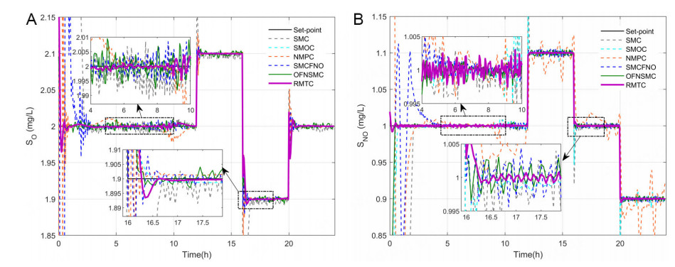
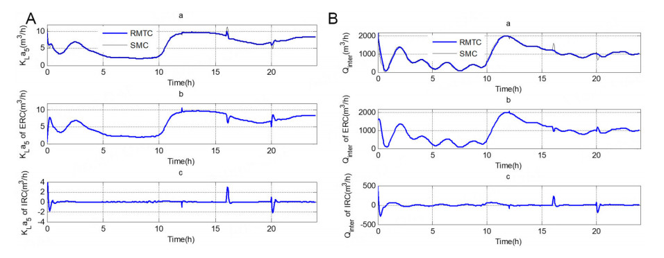
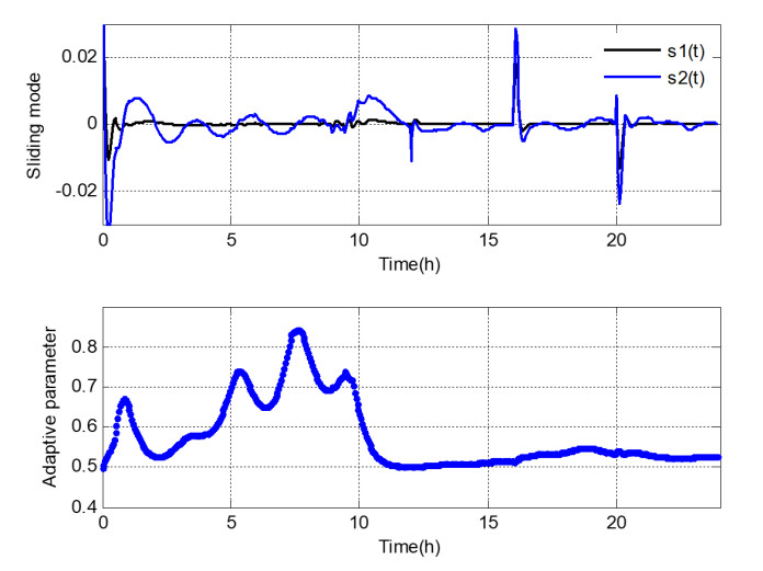
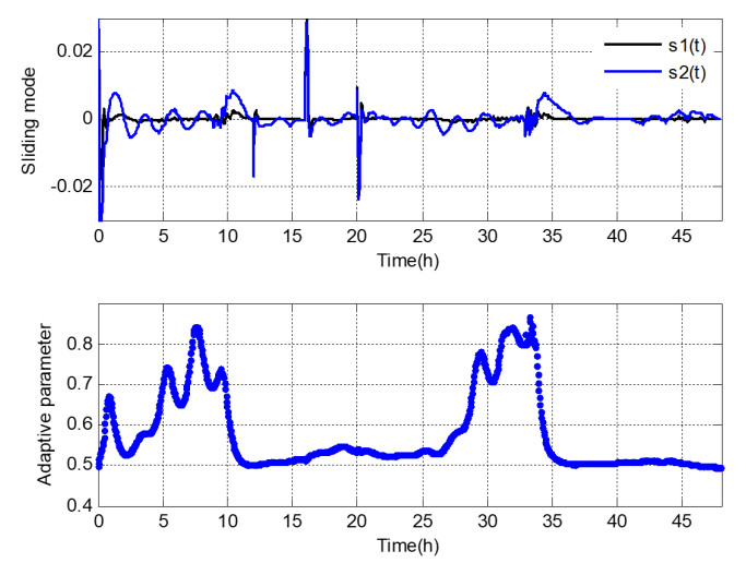
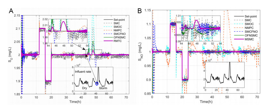
The set-point changes of $$ S_O $$ and $$ S_{NO} $$ are put into the control system to identify its performance. The set-points of $$ S_O $$ are set to 2.0 mg/L from 00:00 to 12:00, 2.1 mg/L from 12:00 to 16:00, 1.9 mg/L from 16:00 to 20:00, 2.0 mg/L from 20:00 to 24:00. The set-points of $$ S_{NO} $$ are set to 1.0 mg/L from 00:00 to 12:00, 1.1 mg/L from 12:00 to 16:00, 1.0 mg/L from 16:00 to 20:00, 0.9 mg/L from 20:00 to 24:00. The initial structure of SOFNN is 2-6-6-2. The initial value $$ \sigma = 2.5 $$ is applied to every hidden neuron. And the initial weights are taken randomly in the interval $$ [-0.5, 0.5] $$. The other controller parameters are: $$ v = 2 $$, $$ \lambda = 6 $$ $$ \delta = 0.16 $$, $$ \eta_1 = \eta_2 = \eta_3 = 0.0121 $$, $$ \kappa_1 = 0.232 $$ and $$ \kappa_2 = 1.215 $$. The results of RMTC are displayed in Figure 4, Figure 5 and Figure 6. In particular, the control results of $$ S_O $$ and $$ S_{NO} $$ are shown in Figure 4. Figure 5 show the control actions of $$ S_O $$ and $$ S_{NO} $$. The dynamic of sliding mode $$ \mathbf{s}(t) $$ and adaptive parameter $$ \varsigma(t) $$ is displayed in Figure 6.

Robust multivariable tracking control for biological wastewater treatment process with external disturbances and uncertainties

Figure 4. (A) Tracking the performance of SO in case Ⅰ; (B) Tracking the performance of SNO in case Ⅰ.

Robust multivariable tracking control for biological wastewater treatment process with external disturbances and uncertainties

Figure 5. (A) (a) The dynamic of KLa5 (m3/h); (b) The dynamic of KLa5 (m3/h) using direct controller; (c) The dynamic of KLa5 (m3/h) using approximate controller. (B)(a)The dynamic of Qinter (m3/h); (b)The dynamic of Qinter (m3/h) using direct controller; (c)The dynamic of Qinter (m3/h) using approximate controller.

Robust multivariable tracking control for biological wastewater treatment process with external disturbances and uncertainties

Figure 6. The dynamic of sliding mode s(t) and adaptive parameter $$ \varsigma(t)$$.

From the graphics in Figure 4, the behavior of the whole system using RMTC is observable (purple line), it is very close to the set points (black line). The control errors of RMTC can be achieved within a small region. In Figure 4, the outputs of RMTC can track the set points too. The curves of control errors of $$ S_{NO} $$ demonstrate that RMTC can obtain small errors in the $$ S_{NO} $$ control. From Figure 5, the control inputs of RMTC tend to be smoother than the control inputs using the direct control and the approximate controller, which means that the chattering problem can be attenuated. In addition, Figure 6 shows that RMTC can find the appropriate values of the adaptive parameter following the dynamic aeration and sludge recycling.

To assess the efficacy of RMTC, its findings are compared with several pioneering works including, the SMC[19], the SMC based on a disturbance observer (SMOC)[28], the NMPC[45], the SMC based on a fuzzy neural network observer (SMCFNO)[34], and the observer-based sliding mode controller with self-structuring FNN (SFNN) identifier (OFNSMC)[35]. The parameters, including the control gains and initial structure of these control methods, are the same as RMTC. Other parameters are defined as in the original paper. The statistical analysis of RMTC and the other controllers is given in Table 1.

Table 1

The comparison of tracking performance

Controller $$ \mathit{\boldsymbol{S_O}} $$ $$ \mathit{\boldsymbol{S_{NO}}} $$ (mg/L)
Num. $$ \mathit{\boldsymbol{E_{IA}}} $$ (mg/L) $$ \mathit{\boldsymbol{E_{ISD}}} $$ (mg/L) $$ \mathit{\boldsymbol{U_{rms}}} $$ (mg/L) Num. $$ \mathit{\boldsymbol{E_{IA}}} $$ (mg/L) $$ \mathit{\boldsymbol{E_{ISD}}} $$ (mg/L) $$ \mathit{\boldsymbol{U_{rms}}} $$ (mg/L)
RMTC 9 0.018 0.032 0.31 8 0.013 0.028 44.9
SMC[19] - 0.728 0.117 0.78 - 0.861 0.980 82.3
SMOC[28] - 0.232 0.058 0.53 - 0.292 0.049 51.2
NMPC[45] - 0.021 0.039 0.45 - 0.614 0.613 82.8
SMCFNO[34] 12 0.031 0.053 0.47 10 0.123 0.044 51.7
OFNSMC[35] 11 0.027 0.049 0.46 10 0.051 0.035 49.7

Compared to SMCFNO and OFNSMC, the proposed RMTC achieves the most compact structure. The smallest $$ IAE $$ and error in Table 1 indicate that the tracking performance of RMTC is the best among these different methods. The smallest $$ E_{IA} $$ and $$ E_{ISD} $$ show that RMTC can realize a preferable response. Therefore, it can be concluded that RMTC can obtain ideal performance concerning dynamic aeration and sludge recycling than the other control strategies. It should be noted that this proposed RMTC demonstrates the robustness. Moreover, the smallest root-mean-square values of control input also indicate that the chattering problem of control action is decreased obviously and the results of RMTC are smoother than the other methods.

Case Ⅱ: The data of the last 48 hours, including the dry and rain conditions, are used to perform the control of aeration and sludge recycle flow rate. The disturbances contain the rain events, as well as the decreasing nitrification and denitrification.

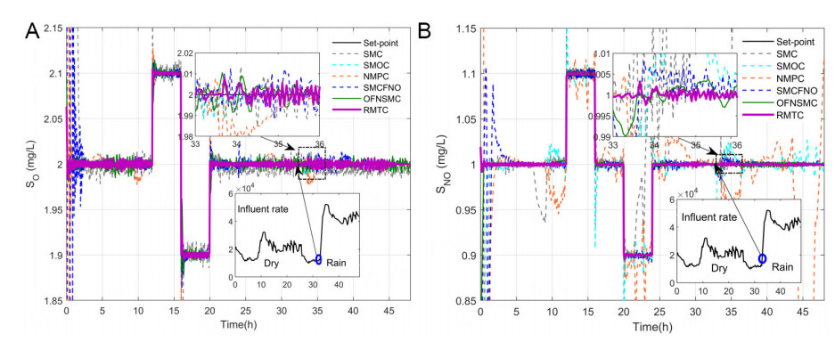
The rain event is at 9:00 on the second day. The decreasing nitrification is denoted by the specific growth rate of autotrophs which changes from 0.5 to 0.63 day$$ ^{-1} $$ with a linear fashion; and the decreasing denitrification is described by the specific growth rate of heterotrophs that ranges from 0.24 to 0.36 day$$ ^{-1} $$ with a linear fashion. Meanwhile, the sensor noise and set-point changes of $$ S_O $$ and $$ S_{NO} $$ are put into the control system according to case Ⅰ.

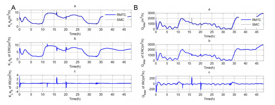
The initial structure of SOFNN is 2-6-6-2. The initial value $$ \sigma = 2.5 $$ is applied to every hidden neuron. Additionally, the initial weights are taken randomly in the interval $$ [-0.5, 0.5] $$. The other parameters are: $$ v = 2 $$, $$ \lambda = 6 $$, $$ \delta = 0.16 $$, $$ \eta_1 = \eta_2 = \eta_3 = 0.0121 $$, $$ \kappa_1 = 0.232 $$ and $$ \kappa_2 = 1.215 $$. The results of RMTC are given in Figure 7, Figure 8 and Figure 9. Figure 7 show the control results of $$ S_O $$ and $$ S_{NO} $$. It can be seen that the curve of $$ S_O $$ and $$ S_{NO} $$ still tracks the set points very well despite the existence of the rain event. The dynamics of $$ K_{La5} $$ and $$ Q_{inter} $$, using RMTC, the direct controller, and the approximate controller, are presented in Figure 8. The curve of control input produced by RMTC tends to be flat, which means that both the control efforts of direct and approximate controllers complement each other to obtain smooth control output. The dynamic of sliding mode $$ \mathbf{s}(t) $$ and adaptive parameter $$ \varsigma(t) $$ is presented in Figure 9, which explains that the adaptive parameter can be achieved following dynamic aeration and sludge recycling.

Robust multivariable tracking control for biological wastewater treatment process with external disturbances and uncertainties

Figure 7. (A) Tracking the performance of SO in case Ⅱ; (B) Tracking the performance of SNO in case Ⅱ.

Robust multivariable tracking control for biological wastewater treatment process with external disturbances and uncertainties

Figure 8. (A) (a) The dynamic of KLa5 (m3/h); (b) The dynamic of KLa5 (m3/h) using direct controller; (c) The dynamic of KLa5 (m3/h) using approximate controller. (B)(a)The dynamic of Qinter (m3/h); (b)The dynamic of Qinter (m3/h) using direct controller; (c)The dynamic of Qinter (m3/h) using approximate controller.

Robust multivariable tracking control for biological wastewater treatment process with external disturbances and uncertainties

Figure 9. The dynamic of sliding mode s(t) and adaptive parameter $$ \varsigma(t)$$.

In addition, the comparison of RMTC with other controllers is given in Table 2. The smallest \(E_{IA}\), \(E_{ISD}\), and \(U_{rms}\) in Table 2 indicate that the tracking performance of RMTC is superior among these methods. Although the accuracy and stability are influenced by the rain event, uncertainties, sensor noise, and set-point changes, the output of RMTC remains precise and stable with the least fuzzy rules. In addition, because the set points are maintained well, the smallest \(E_{IA}\) and \(E_{ISD}\) in Table 2 demonstrate that RMTC has a preferable response. Consequently, RMTC exhibits superior control performance in dynamic aeration and sludge recycling compared to other approaches.

Table 2

The comparison of tracking performance

Controller $$ \mathit{\boldsymbol{S_O}} $$ $$ \mathit{\boldsymbol{S_{NO}}} $$ (mg/L)
Num. $$ \mathit{\boldsymbol{E_{IA}}} $$ (mg/L) $$ \mathit{\boldsymbol{E_{ISD}}} $$ (mg/L) $$ \mathit{\boldsymbol{U_{rms}}} $$ (mg/L) Num. $$ \mathit{\boldsymbol{E_{IA}}} $$ (mg/L) $$ \mathit{\boldsymbol{E_{ISD}}} $$ (mg/L) $$ \mathit{\boldsymbol{U_{rms}}} $$ (mg/L)
RMTC 10 0.058 0.047 0.21 9 0.014 0.017 42.9
SMC[19] - 0.663 0.532 0.69 - 4.361 3.488 105.0
SMOC[28] - 0.263 0.218 0.56 - 0.434 0.508 82.5
NMPC[45] - 0.119 0.098 0.32 - 0.528 0.711 79.7
SMCFNO[34] 14 0.108 0.105 0.47 12 0.137 0.404 64.8
OFNSMC[35] 12 0.076 0.048 0.35 11 0.047 0.103 50.1

Case Ⅲ: In this case, the data of the last 72 h is used to analyze the control of aeration and sludge recycle flow rate. The influent disturbances include the rain and storm events, the decreasing nitrification and the decreasing denitrification, as well as the set-point changes and measurement noises.

The rain and storm events are launched from 9:00 to 20:30 on the second day, respectively. The decreasing nitrification and the decreasing denitrification are shaped according to case Ⅱ. The set-points are provided the same as in case Ⅰ.

The random measurement noises are set to the range of $$ [-0.017, 0.017] $$. As to self-organizing FNN, the structure is initialized as 2-6-6-2, and the weights $$ \mathbf{w} $$ are taken randomly in the interval $$ [-0.5, 0.5] $$. The initial value $$ \sigma= $$ 2.5 is applied to every hidden neuron of SOFNN. The other controller parameters are chosen as: $$ v= $$ 0.26, $$ \lambda= $$ 5, $$ \delta= $$ 0.18, $$ \eta_1 $$ = $$ \eta_2 $$ = $$ \eta_3 $$ = 0.0078, $$ \kappa_1 $$ = 0.317 and $$ \kappa_2 $$ = 2.905.

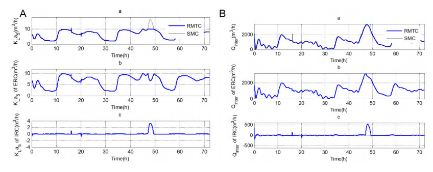
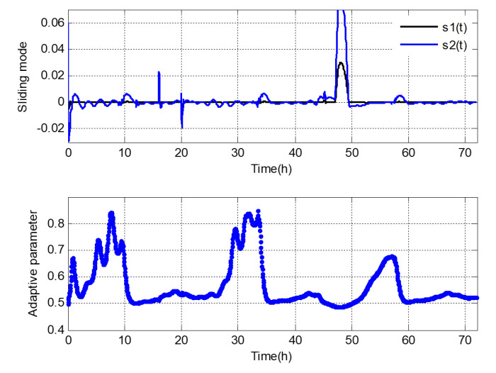
The experiment results are presented in Figure 10, Figure 11 and Figure 12. Figure 10 shows that the curves of $$ S_O $$ and $$ S_{NO} $$ track the set points under the condition of serious rain and storm events. It can be noticed that the behavior of RMTC, even if large disturbances, remains satisfactory. Compared to SMC, in Figure 11, the control inputs of RMTC associated with $$ K_{La5} $$ and $$ Q_{inter} $$ tend to be smoother than the control inputs of the direct controller or the approximate controller. It proves that the chattering has been attenuated by the adaptive strategy of RMTC. Furthermore, according to Figure 12, the sliding mode $$ \mathbf{s}(t) $$ and the adaptive parameter of RMTC can be self-tuned following dynamic aeration and sludge recycling.

Robust multivariable tracking control for biological wastewater treatment process with external disturbances and uncertainties

Figure 10. (A) Tracking the performance of SO in case Ⅲ; (B) Tracking the performance of SNO in case Ⅲ.

Robust multivariable tracking control for biological wastewater treatment process with external disturbances and uncertainties

Figure 11. (A) (a) The dynamic of KLa5 (m3/h); (b) The dynamic of KLa5 (m3/h) using direct controller; (c) The dynamic of KLa5 (m3/h) using approximate controller. (B)(a)The dynamic of Qinter (m3/h); (b)The dynamic of Qinter (m3/h)using direct controller; (c)The dynamic of Qinter (m3/h) using approximate controller.

Robust multivariable tracking control for biological wastewater treatment process with external disturbances and uncertainties

Figure 12. The dynamic of sliding mode s(t) and adaptive parameter $$ \varsigma(t)$$.

The details of the comparisons in terms of $$ Num. $$, $$ E_{IAE} $$, $$ E_{ISD} $$, and $$ U_{rms} $$ are shown in Table 3. The least $$ Num. $$, $$ E_{IA} $$ and $$ E_{ISD} $$ are obtained by RMTC compared to other control strategies. The values of $$ E_{IA} $$ vary from 0.030 mg/L to 0.040 mg/L under different scenarios. These results indicate that the proposed RMTC holds high-quality tracking performance and robustness against the disturbances. Consequently, the proposed RMTC in this case exhibits superior control performance for dynamic aeration and sludge recycling compared to other control techniques.

Table 3

The comparison of tracking performance

Controller $$ \mathit{\boldsymbol{S_O}} $$ $$ \mathit{\boldsymbol{S_{NO}}} $$ (mg/L)
Num. $$ \mathit{\boldsymbol{E_{IA}}} $$ (mg/L) $$ \mathit{\boldsymbol{E_{ISD}}} $$ (mg/L) $$ \mathit{\boldsymbol{U_{rms}}} $$ (mg/L) Num. $$ \mathit{\boldsymbol{E_{IA}}} $$ (mg/L) $$ \mathit{\boldsymbol{E_{ISD}}} $$ (mg/L) $$ \mathit{\boldsymbol{U_{rms}}} $$ (mg/L)
RMTC 10 0.038 0.037 0.191 9 0.017 0.052 31.4
SMC[19] - 0.812 0.552 0.572 - 0.705 0.943 51.8
SMOC[28] - 0.154 0.107 0.491 - 0.473 0.504 42.1
NMPC[45] - 0.087 0.065 0.262 - 4.870 2.551 66.3
SMCFNO[34] 15 0.231 0.099 0.459 13 0.150 0.150 41.2
OFNSMC[35] 11 0.069 0.066 0.350 12 0.056 0.103 39.8

4.3. Analysis of experimental results

The experiments are performed to demonstrate the viability of RMTC for WWTP. The dynamic nature of WWTP is characterized by diverse physical and biological processes with significant external disturbances, complicating the regulation of $$ S_O $$ and $$ S_{NO} $$ in BWWTP. Therefore, RMTC can obtain superior control performance associated with $$ E_{IAE} $$, $$ E_{ISD} $$, and $$ U_{rms} $$ in different cases (see Figure 4, Figure 7 and Figure 10). Furthermore, the results in Table 1, Table 2 and Table 3 demonstrate that RMTC can effectively suppress the external disturbances and uncertainties. Although the chattering problem derived from the introduction of SMC impedes its application, RMTC still suppresses the oscillation of control input with the design of SOFNN and further maintains the smoothness of performance. An adaptive technique is developed to enhance the adaptive capacity to mitigate the chattering phenomenon and maintain steady-state control performance.

5. CONCLUSIONS

In this study, an RMTC is designed to realize an effective control performance for BWWTP. The outcomes of experiments have shown that RMTC is effective. The results show that RMTC performs better than other control methods. The accuracy and smoothness of control output can be improved for the BWWTP. The details can be summarized as follows:

(1) This proposed RMTC can provide a framework to improve the robust performance for tracking multiple variables. This control strategy can obtain good robustness for both the external disturbances and uncertainties of BWWTP.

(2) The control gain of RMTC, adjusted by an adaptive strategy with both the direct controller and the approximate controller, can maintain the steady-state control performance under different operational conditions.

(3) Sufficient conditions and parameters are provided for RMTC based on the stability analysis, which allows the proposed RMTC to be applied in the real BWWTP. Experimental experiments demonstrate that RMTC is an effective instrument for BWWTP.

Furthermore, the proposed RMTC will be applied to different kinds of BWWTP and other fields.

DECLARATIONS

Acknowledgments

The authors would like to express our great appreciation to the editors and reviewers.

Authors' contributions

Made substantial contributions to conception and design of the study and performed data analysis and interpretation: Wu, X.; Han, W.; Yang, H.; Han, H.

Performed data acquisition and provided administrative, technical, and material support: Qiao, J.; Peng, X.

Availability of data and materials

The experimental dataset supporting this study can be obtained from "Benchmark simulation model no. 1 (BSM1)". The implementation of BSM1 is available here: https://portal.research.lu.se/en/publications/benchmark-simulation-model-no-1-bsm1.

Financial support and sponsorship

This work was supported by National Science Foundation of China under Grants 62422301, 62125301, 62021003, and 62103011, Beijing Natural Science Foundation under Grants L253010, National Key Research and Development Project under Grants 2022YFB3305800-05, and Youth Beijing Scholar under Grant No. 037.

Conflicts of interest

Han, H. is Editorial Board Member of the journal Complex Engineering Systems. Han, H. was not involved in any steps of editorial processing, notably including reviewers' selection, manuscript handling and decision making, while the other authors have declared that they have no conflicts of interest.

Ethical approval and consent to participate

Not applicable.

Consent for publication

Not applicable.

Copyright

© The Author(s) 2025.

REFERENCES

1. Li, D.; Yan, Y.; Li, D. Adaptive event-triggered control for wastewater treatment process using self-organizing fuzzy neural network. IEEE. Trans. Autom. Sci. Eng. 2011, 22, 11333-42.

2. Alharbi, M.; Hong, P.; Laleg-Kirati, T. M. Sliding window neural network-based sensing of bacteria in wastewater treatment plants. J. Process. Control. 2022, 110, 35-44.

3. Li, L.; Gu, T.; Pan, H.; Hu, J.; Yu, X. Sensor and actuator fault estimations and self-healing control of discrete-time t-s fuzzy model with double observers and its application to wastewater treatment process. IEEE. Trans. Fuzzy. Syst. 2024, 32, 2428-37.

4. Cao, W.; Yang, Q.; Meng, W.; Xie, S. Data-based robust adaptive dynamic programming for balancing control performance and energy consumption in wastewater treatment process. IEEE. Trans. Ind. Inform. 2023, 20, 6622-30.

5. Santín, I.; Barbu, M.; Pedret, C.; Vilanova, R. Control strategies for nitrous oxide emissions reduction on wastewater treatment plants operation. Water. Res. 2017, 125, 466-77.

6. Du, P.; Zhong, W.; Peng, X.; Li, L.; Wu, X. Residual-triggered threshold decision and performance self-healing control for wastewater treatment process. Inf. Sci. 2023, 64, 118822.

7. Yu, X.; Shen, Y.; Guo, Z.; et al. Intelligent aeration amount prediction control for wastewater treatment process based on recurrent neural network. J. Franklin. Inst. 2024, 361, 107276.

8. Hvala, A. N.; Kocijan, B. J. Input variable selection using machine learning and global sensitivity methods for the control of sludge bulking in a wastewater treatment plant. Comput. Chem. Eng. 2021, 154, 107493.

9. Asteriadis, I.; Azis, K.; Ntougias, S.; Melidis, P. A control strategy for an intermittently aerated and fed bioreactor to reduce aeration costs: a simulation study. Biochem. Eng. J. 2021, 173, 108081.

10. Floresestrella, R.; Quiroz, G.; Mendezacosta, H. O. H control of anaerobic digester for winery industry wastewater treatment. Ind. Eng. Chem. Res. 2013, 52, 2625-32.

11. Vangsgaard, A. K.; Mauricio, M. I.; Gernaey, K.; Sin, G. Development of novel control strategies for single-stage autotrophic nitrogen removal: A process oriented approach. Comput. Chem. Eng. 2014, 66, 71-81.

12. Petre, E.; Teanu, D. A multivariable robust-adaptive control strategy for a recycled wastewater treatment bioprocess. Chem. Eng. Sci. 2013, 90, 40-50.

13. Chen, G.; Xia, J.; Park, J. H.; Shen, H.; Zhuang, G. Robust sampled-data control for switched complex dynamical networks with actuators saturation. IEEE. Trans. Cybern. 2022, 52, 10909-23.

14. Mu, C.; Wang, K.; Qiu, T. Dynamic Event-Triggering neural learning control for partially unknown nonlinear systems. IEEE. Trans. Cybern. 2022, 52, 2200-2213.

15. Mohseni, S. S.; Babaeipour, V.; Vali, A. R. Design of sliding mode controller for the optimal control of fed-batch cultivation of recombinant E. coli. Chem. Eng. Sci. 2009, 64, 4433-41.

16. Levant, A. Chattering analysis. IEEE. Trans. Autom. Control. 2010, 55, 1380-89.

17. Liu, C.; Wen, G.; Zhao, Z.; Sedaghati, R. Neural-network-based sliding-mode control of an uncertain robot using dynamic model approximated switching gain. IEEE. Trans. Cybern. 2021, 51, 2339-46.

18. Rios, H.; Falcon, R.; Gonzalez, O. A.; Dzul, A. E. Continuous sliding-modes control strategies for quad-rotor robust tracking: real-time application. IEEE. Trans. Ind. Electron. 2019, 66, 1264-72.

19. Selisteanu, D.; Petre, E.; Rasvan, V. B. Sliding mode and adaptive sliding-mode control of a class of nonlinear bioprocesses. Int. J. Adapt. Control. Signal. Process. 2007, 21, 795-822.

20. Petre, E.; Teanu, D.; Sendrescu, D. Adaptive and robust-adaptive control strategies for anaerobic wastewater treatment bioprocesse. Chem. Eng. J. 2013, 217, 363-78.

21. Wei, W.; Chen, N.; Zhang, Z.; et al. A scalable-bandwidth extended state observer-based adaptive sliding-mode control for the dissolved oxygen in a wastewater treatment process. IEEE. Trans. Cybern. 2021, 52, 13448-57.

22. Liu, Q.; Jiang, X.; Qi, N.; Li, M. Sliding mode variable structure control for wastewater treatment based on an improved linear extended observer. J. Water. Process. Eng. 2024, 68, 106435.

23. Mateusz, C.; Rafal, L. A robust sliding mode observer for non-linear uncertain biochemical systems. ISA. Trans. 2022, 123, 25-45.

24. Pan, H.; Yu, X.; Hu, J.; et al. A self-healing controller based on sliding-mode control for sensor fault in wastewater treatment processes. IEEE. J. Process. Control. 2023, 127, 102997.

25. Faisal, M.; Muttaqi, K. M.; Sutanto, D.; et al. Control technologies of wastewater treatment plants: The state-of-the-art, current challenges, and future directions. Renew. Sustain. Energy. Rev. 2023, 181, 113324.

26. Fida, T.; Samah, B. A.; Anis, M.; Ridha, B. A. An interval multiobserver for nonlinear systems subject to internal and external disturbances: Real time experimental validation. J. Process. Control. 2022, 116, 199-208.

27. Zúniga, I. T.; Queinnec, I.; Wouwer, A. V. Observer-based output feedback linearizing control strategy for a nitrification–denitrification biofilter. Chem. Eng. J. 2012, 191, 243-55.

28. Gonzalez, J.; Fernandez, G.; Aguilar, R. Sliding mode observer-based control for a class of bioreactors. Chem. Eng. J. 2001, 83, 25-32.

29. Wahab, N. A.; Katebi, R.; Balderud, J. Data-driven adaptive model-based predictive control with application in wastewater systems. IET. Control. Theory. Appl. 2011, 5, 803-12.

30. Samuelsson, P.; Halvarsson, B.; Carlsson, B. Interaction analysis and control structure selection in a wastewater treatment plant model. IEEE. Trans. Control. Syst. Technol. 2005, 13, 955-64.

31. Zhang, S.; Zhou, P.; Xie, Y.; Chai, T. Improved model-free adaptive predictive control method for direct data-driven control of a wastewater treatment process with high performance. J. Process. Control. 2022, 110, 11-23.

32. Li, H.; Yu, J.; Hilton, C. Adaptive sliding-mode control for nonlinear active suspension vehicle systems using T-S fuzzy approach. IEEE. Trans. Ind. Electron. 2013, 60, 3328-38.

33. Wang, D.; Zhao, M.; Ha, M.; Ren, J. Neural optimal tracking control of constrained nonaffine systems with a wastewater treatment application. Neural. Netw. 2021, 143, 121-32.

34. Su, Y.; Xu, L.; Li, D. Adaptive fuzzy control of a class of MIMO nonlinear system with actuator saturation for greenhouse climate control problem. IEEE. Trans. Autom. Sci. Eng. 2016, 13, 772-88.

35. de Canete, J. F.; del Saz-Orozco, P.; Gómez-de Gabriel, J.; et al. Control and soft sensing strategies for a wastewater treatment plant using a neuro-genetic approach. Comput. Chem. Eng. 2021, 144, 107146.

36. Lei, Y.; Ding, L.; Zhang, W. Generalization performance of radial basis function networks. IEEE. Trans. Neural. Netw. Learn. Syst. 2015, 26, 551-64.

37. Lin, M.; Luo, F. Adaptive neural control of the dissolved oxygen concentration in WWTPs based on disturbance observer. Neurocomputing. 2016, 185, 133-41.

38. Huang, M.; Wan, J.; Ma, Y.; Wang, Y. Control rules of aeration in a submerged biofilm wastewater treatment process using fuzzy neural networks. Expert. Syst. Appl. 2009, 36, 10428-37.

39. Chen, W.; Chang, N.; Chen, J. Rough set-based hybrid fuzzy-neural controller design for industrial wastewater treatment. Water. Res. 2003, 37, 95-107.

40. Bououden, S.; Chadli, M.; Karimi, H. R. Control of uncertain highly nonlinear biological process based on Takagi-Sugeno fuzzy models. Signal. Process. 2015, 108, 195-205.

41. Huang, M.; Wan, J.; Hu, K.; Ma, Y.; Wang, Y. Enhancing dissolved oxygen control using an on-line hybrid fuzzy-neural soft-sensing model-based control system in an anaerobic/anoxic/oxic process. J. Ind. Microbiol. Biotechnol. 2013, 40, 1393-401.

42. Ruan, J.; Zhang, C.; Li, Y.; et al. Improving the efficiency of dissolved oxygen control using an on-line control system based on a genetic algorithm evolving FWNN software sensor. J. Environ. Manag. 2017, 187, 550-59.

43. Xu, B.; Li, Y.; Hou, Z.; Ahn, C. K. Dynamic event-triggered reinforcement learning-based consensus tracking of nonlinear multi-agent systems. IEEE. Trans. Circuits. Syst. I. Regul. Pap. 2023, 70, 2120-32.

44. Xu, B.; Li, Y. Prescribed-time fully distributed Nash equilibrium seeking of nonlinear multi-agent systems over unbalanced digraphs. Automatica. 2024, 169, 111847.

45. Han, H.; Qiao, J. Nonlinear model-predictive control for industrial processes: An application to wastewater treatment process. IEEE. Trans. Ind. Electron. 2014, 61, 1970-82.

Cite This Article

Research Article
Open Access
Robust multivariable tracking control for biological wastewater treatment process with external disturbances and uncertainties

How to Cite

Download Citation

If you have the appropriate software installed, you can download article citation data to the citation manager of your choice. Simply select your manager software from the list below and click on download.

Export Citation File:

Type of Import

Tips on Downloading Citation

This feature enables you to download the bibliographic information (also called citation data, header data, or metadata) for the articles on our site.

Citation Manager File Format

Use the radio buttons to choose how to format the bibliographic data you're harvesting. Several citation manager formats are available, including EndNote and BibTex.

Type of Import

If you have citation management software installed on your computer your Web browser should be able to import metadata directly into your reference database.

Direct Import: When the Direct Import option is selected (the default state), a dialogue box will give you the option to Save or Open the downloaded citation data. Choosing Open will either launch your citation manager or give you a choice of applications with which to use the metadata. The Save option saves the file locally for later use.

Indirect Import: When the Indirect Import option is selected, the metadata is displayed and may be copied and pasted as needed.

About This Article

© The Author(s) 2025. Open Access This article is licensed under a Creative Commons Attribution 4.0 International License (https://creativecommons.org/licenses/by/4.0/), which permits unrestricted use, sharing, adaptation, distribution and reproduction in any medium or format, for any purpose, even commercially, as long as you give appropriate credit to the original author(s) and the source, provide a link to the Creative Commons license, and indicate if changes were made.

Data & Comments

Data

Views
18
Downloads
2
Citations
0
Comments
0
1

Comments

Comments must be written in English. Spam, offensive content, impersonation, and private information will not be permitted. If any comment is reported and identified as inappropriate content by OAE staff, the comment will be removed without notice. If you have any queries or need any help, please contact us at [email protected].

0
Download PDF
Share This Article
Scan the QR code for reading!
See Updates
Contents
Figures
Related
Complex Engineering Systems
ISSN 2770-6249 (Online)

Portico

All published articles are preserved here permanently:

https://www.portico.org/publishers/oae/

Portico

All published articles are preserved here permanently:

https://www.portico.org/publishers/oae/