

A knowledge-distilled artificial neural network constitutive model for finite element simulation of hot-deformed β-C titanium alloy
 0
Graphical Abstract
Abstract
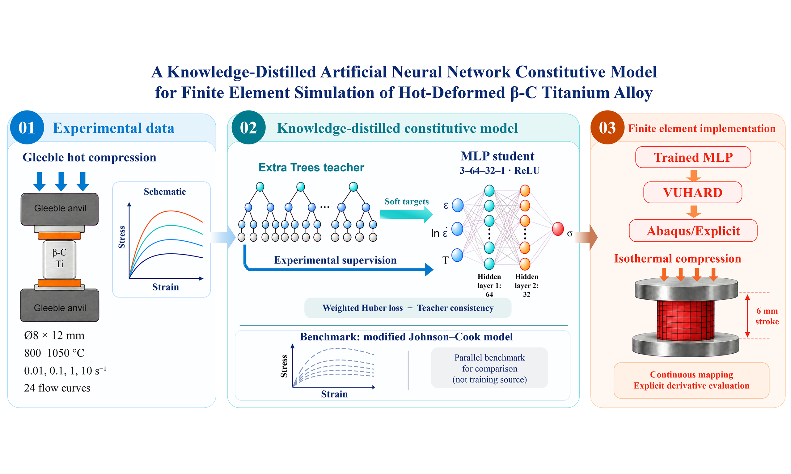
Accurate, computationally deployable constitutive models are required for reliable finite element (FE) simulations of metallic hot deformation. This study develops a knowledge-distilled artificial neural network (KD-ANN) constitutive model for β-C titanium alloy using 24 flow-stress curves measured at 800-1,050 °C and strain rates of 0.01-10 s-1. An Extra Trees model serves as the teacher, while a compact multilayer perceptron provides a continuous constitutive mapping with explicit derivative evaluation for FE implementation. The student is trained using experimental and teacher supervision, weighted Huber loss, curve-balanced weighting and enhanced weighting in the low-strain region. Following preliminary teacher-algorithm and student-configuration screening, temperature-wise predictive performance is evaluated using curve-grouped leave-one-temperature-out validation. In each fold, all four curves at the target temperature are held out, while the fold-specific KD-ANN and modified Johnson–Cook (J–C) models are fitted using only the retained temperature conditions. Across the six held-out-temperature folds, KD-ANN achieves mean values of the coefficient of determination = 0.984, root mean square error = 11.40 MPa and mean absolute error (MAE) = 9.21 MPa, compared with 0.960, 17.12 and 12.58 MPa, respectively, for the modified J–C model. Sequential ablation and targeted control experiments show that the joint use of experimental stresses and teacher-generated targets produces the largest incremental improvement within the tested training framework. The trained student network is implemented in Abaqus through a VUHARD user subroutine. For the fold in which the lower-boundary temperature of 800 °C is held out from model fitting and validation, the FE load–displacement predictions yield a mean MAE of 0.729 kN, compared with 1.213 kN for the modified J–C model. These results demonstrate improved prediction of complete flow curves at unseen temperatures within the investigated range and support the use of KD-ANN as a constitutive input for hot-compression simulations.
Keywords


 Download PDF
INTRODUCTION
High-strength near-β titanium alloys are increasingly used in aerospace structures because they combine high specific strength, good fatigue resistance, and attractive damage tolerance under demanding service conditions[1-5]. Among them, β-C (Ti-3Al-8V-6Cr-4Mo-4Zr) is a representative high-strength alloy for heavily loaded forged and rolled components[6,7]. However, its hot workability is highly sensitive to deformation temperature, strain, and strain rate, so a narrow process window may readily lead to unstable flow, microstructural heterogeneity, and property fluctuations[8-10]. During hot deformation, work hardening, dynamic recovery (DRV), and thermally activated softening evolve concurrently, giving rise to a strongly nonlinear flow response[11,12]. Therefore, an accurate constitutive description is a prerequisite for reliable finite element (FE) simulation, process optimization, and microstructure control during hot compression, forging, and rolling of this alloy.
Phenomenological constitutive models such as Arrhenius-type, Zener–Hollomon (Z–H), and Johnson–Cook (J–C) models remain the most widely used approaches in thermomechanical simulation because of their compact forms and relatively convenient calibration procedures[13-19]. Nevertheless, their predefined analytical structures inevitably simplify the coupling among strain, strain rate, and temperature. When deformation conditions span a broad range or when local softening behavior becomes pronounced, fixed-form constitutive models may fail to reproduce the detailed evolution of flow curves, and parameter identification can become sensitive to data dispersion and fitting strategy. Even recent efforts to improve parameter-identification procedures or optimize J–C constants for titanium alloys still remain within the framework of prescribed constitutive models, which limits their flexibility in describing complex nonlinear responses across the full processing domain[20].
In this context, artificial neural network (ANN) constitutive models have attracted growing attention because they can learn nonlinear mappings directly from experimental data without imposing a rigid functional form in advance[21-24]. Previous studies have demonstrated that ANN-based models can predict flow stress more accurately than conventional constitutive models for magnesium alloys, titanium alloys, and Al-Zn-Mg alloys under hot-working conditions[25]. More recent machine-learning studies on complex alloys have further confirmed that data-driven models can achieve markedly improved predictive accuracy over traditional approaches when evaluated by standard statistical metrics[26,27]. In constitutive modeling, ANN-based models exhibit excellent fitting capability. More importantly, they are capable of capturing the complex couplings among thermomechanical variables, which are difficult to be analytically described by conventional phenomenological constitutive models.
Despite these advantages, a conventional ANN trained only by minimizing pointwise stress error does not automatically satisfy the requirements of a high-quality constitutive law for process simulation[28,29]. First, numerical agreement in stress magnitude does not guarantee correct local slope evolution, even though the local slope of the flow curve is closely related to the competition between strain hardening and flow softening. Second, the constitutive model must be continuous, numerically stable, portable, and equipped with a consistent procedure for derivative evaluation if it is to be embedded into FE user subroutines. Pantalé et al. showed that ANN flow laws can be implemented efficiently in Abaqus/Explicit, but such implementation places stringent requirements on derivative evaluation and parameter portability[30]. Accordingly, the central challenge is not merely to build a more accurate regressor, but to construct an ANN constitutive model that simultaneously offers high fidelity, physical consistency, and engineering deployability. This challenge is especially relevant for β-C titanium alloy. A recent physics-aided machine-learning study on β-C titanium alloy demonstrated that combining data-driven learning with constitutive knowledge can significantly improve predictive accuracy and generalizability over conventional hot-deformation models. At the same time, recent work[10] on β-C titanium alloy developed a physics-aided machine-learning framework that combines the Z–H equation with a neural network to improve the predictive accuracy and generalization of constitutive analysis, further demonstrating the potential of integrating physical constitutive knowledge with machine learning. However, for practical forming simulation, there remains a clear need for an ANN constitutive framework that not only improves prediction accuracy, but also preserves the compactness, differentiability, and robustness compactness, explicit derivative evaluation, and robustness required for direct FE implementation.
To address this need, the present study develops a knowledge-distilled ANN (KD-ANN) constitutive framework for the hot deformation of β-C titanium alloy based on Gleeble compression data. A knowledge distillation strategy is employed so that a compact student network can inherit the fidelity of a more expressive teacher model in capturing local responses while retaining the continuity, explicit derivative evaluation, and parameter portability required for constitutive embedding. In this way, the proposed model is designed to outperform conventional phenomenological equations and baseline ANN formulations not only in stress prediction, but also in curve-shape fidelity, physical plausibility, and numerical robustness. On this basis, the trained KD-ANN is exported as a constitutive kernel for finite-element simulation and compared with a conventional J–C model to assess its engineering applicability. The objective of this work is therefore twofold: to establish a high-accuracy and FE-friendly ANN constitutive model for β-C titanium alloy, and to demonstrate that this new model can provide a more reliable material description for finite-element simulation. The present study is expected to offer a practical route for bridging advanced data-driven constitutive modeling and process-level simulation, thereby supporting the optimization of hot-deformation process parameters for high-strength titanium alloys.
MATERIALS AND METHODS
The β-C titanium alloy studied in this paper was provided by the Institute of Metal Research, Chinese Academy of Sciences. The original ingot of the alloy was prepared by the vacuum arc remelting (VAR) process, and after cogging, it was further processed into cylindrical specimens with a diameter of
The composition of β-C titanium alloy (mass fraction, %)
| Ti | Al | V | Cr | Mo | Zr | C | O | H | N |
| Bal. | 3.46 | 8.08 | 6.04 | 3.94 | 3.92 | 0.02 | 0.10 | 0.001 | 0.014 |
As shown in Figure 1, the initial microstructure displays a typical equiaxed-β grain structure, where high-angle grain boundaries (HAGBs) dominate the grain boundaries, while low-angle grain boundaries (LAGBs) are rarely observed.
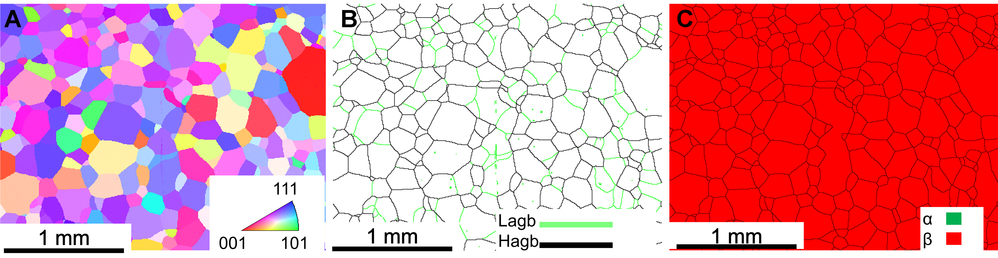
Figure 1. Initial microstructure of specimen: (A) the inverse pole figure map, (B) grain-boundary map and (C) phase map.
In this study, isothermal hot-compression tests were conducted on a Gleeble 3800 thermomechanical simulator to obtain the flow curves of the β-C titanium alloy under different deformation conditions. Graphite foil was placed between the specimen end faces and anvils to minimize interfacial friction. Spot-welded thermocouples were attached to the specimens for real-time temperature monitoring. Under vacuum conditions, the specimens were heated to the prescribed deformation temperatures at a rate of 5 °C/s and held for 300 s prior to deformation to ensure temperature homogenization. The deformation temperatures ranged from 800 to 1,050 °C at 50 °C intervals, and four strain rates of 0.01, 0.1, 1, and 10 s-1 were employed. Each specimen was compressed to a 50% reduction in height. Subsequently, the true stress-strain curves were obtained, and the J–C model and the KD-ANN constitutive model were constructed respectively for fitting analysis of these curves. The established J–C model, KD-ANN model and the specific fitting procedure will be elaborated in detail in Section “RESULTS AND DISCUSSION” below.
The hot compression simulation was performed in Abaqus/Explicit under quasi-static conditions. In this case, the specimen was modeled under isothermal and quasi-static conditions, with the temperature assumed to remain spatially uniform and constant throughout deformation. The deformation field was determined by the FE solution rather than prescribed to be uniform, and thermal effects such as heat conduction, convection, and radiation were neglected. Abaqus/Explicit solves the dynamic equilibrium equations. Under the quasi-static loading condition adopted in this study, inertial effects were assumed to be negligible, and the mechanical response can therefore be approximated by the static equilibrium equation:
The total strain can be decomposed into elastic strain, plastic strain and thermal strain.
ε = εⅇ + εp + εt (2)
where ε, εⅇ, εp and εt represent the total strain tensor, elastic strain tensor, plastic strain tensor and thermal strain tensor, respectively. Plastic yielding was expressed by the von Mises yield criterion
f = σeq - σy ≤ 0, σeq =
where f is the yield function, σeq is the equivalent stress, σy is the yield stress, and s is the deviatoric stress tensor. Under the ideal hot compression condition, the temperature was assumed to remain spatially uniform and constant throughout the deformation process.
RESULTS AND DISCUSSION
Target dataset
Figure 2 presents the flow curves of β-C alloy obtained by the hot compression tests. The flow curves displayed similar shapes over the investigated temperature range. At the onset of deformation, the flow stress increased rapidly with strain. This increase is mainly associated with work hardening caused by dislocation accumulation and interactions. With further straining, thermally activated recovery and recrystallization increasingly offset work hardening. The flow stress therefore declined after reaching the peak stress and gradually approached a quasi-steady state. This post-peak softening is consistent with the occurrence of dynamic recovery and dynamic recrystallization (DRX)[31-33]. Our previous microstructural and electron backscatter diffraction (EBSD) analyses of the β-C alloy provided direct evidence for these softening processes. Post-deformation microstructures, grain-boundary misorientation distributions, and dislocation-density analyses identified DRV and DRX as important mechanisms during hot deformation. The relative contributions of discontinuous dynamic recrystallization (DDRX) and continuous dynamic recrystallization (CDRX) varied with strain rate: higher strain rates promote the occurrence of CDRX, while DDRX dominates under relatively low strain-rate conditions. At a given strain rate and strain, the flow stress decreased with increasing deformation temperature. Elevated temperatures promote dislocation annihilation and rearrangement, as well as recovery and recrystallization. These processes reduce the resistance to plastic deformation and account for the lower flow stress. The abrupt terminal decrease observed at 10 s-1 results from rapid deceleration and unloading of the Gleeble actuator near the prescribed displacement, rather than from intrinsic material softening. Therefore, this terminal unloading segment is excluded from model training and quantitative evaluation.
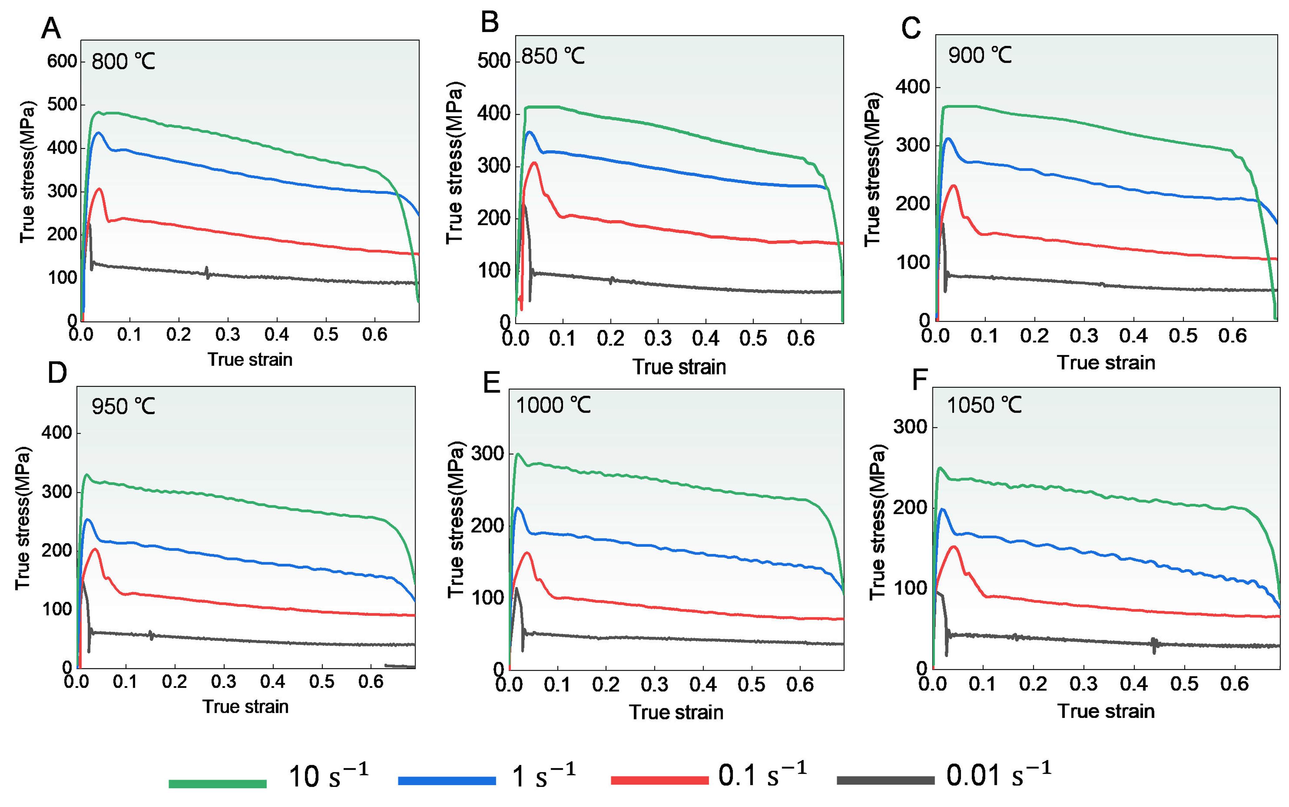
Figure 2. Flow curves under different experimental conditions: (A) 800 °C, (B) 850 °C, (C) 900 °C, (D) 950 °C, (E) 1,000 °C, (F) 1,050 °C.
Overall architecture of the KD-ANN
The flow stress of the β-C titanium alloy during hot compression is jointly governed by strain, strain rate, and deformation temperature, and is further influenced by the coupled effects of work hardening, DRV, and DRX. Consequently, its stress response exhibits pronounced nonlinear characteristics. Therefore, a constitutive model suitable for finite-element implementation in the present study should satisfy three essential requirements. First, it should accurately predict the flow-stress level over a wide range of hot-deformation conditions. Second, it should adequately preserve the local features of the flow curves, particularly the stress evolution during the low-strain regime and the subsequent softening stage. Third, the model should provide a continuous stress response and an explicit procedure for evaluating the required partial derivatives, facilitating implementation in the VUHARD user subroutine of Abaqus/Explicit.
Based on the above considerations, this study adopts a modeling strategy that combines a high-accuracy teacher model with a deployable student model, as schematically illustrated in Figure 3. An Extra Trees model, which exhibits superior pointwise prediction capability, is then introduced as the teacher model to capture complex local response characteristics. Subsequently, knowledge distillation is employed to transfer the local structural information learned by the teacher model to a compact feedforward multilayer perceptron (MLP) student model. This strategy transfers the teacher predictions to a compact student network that provides a continuous stress mapping and explicit derivative evaluation for FE implementation.
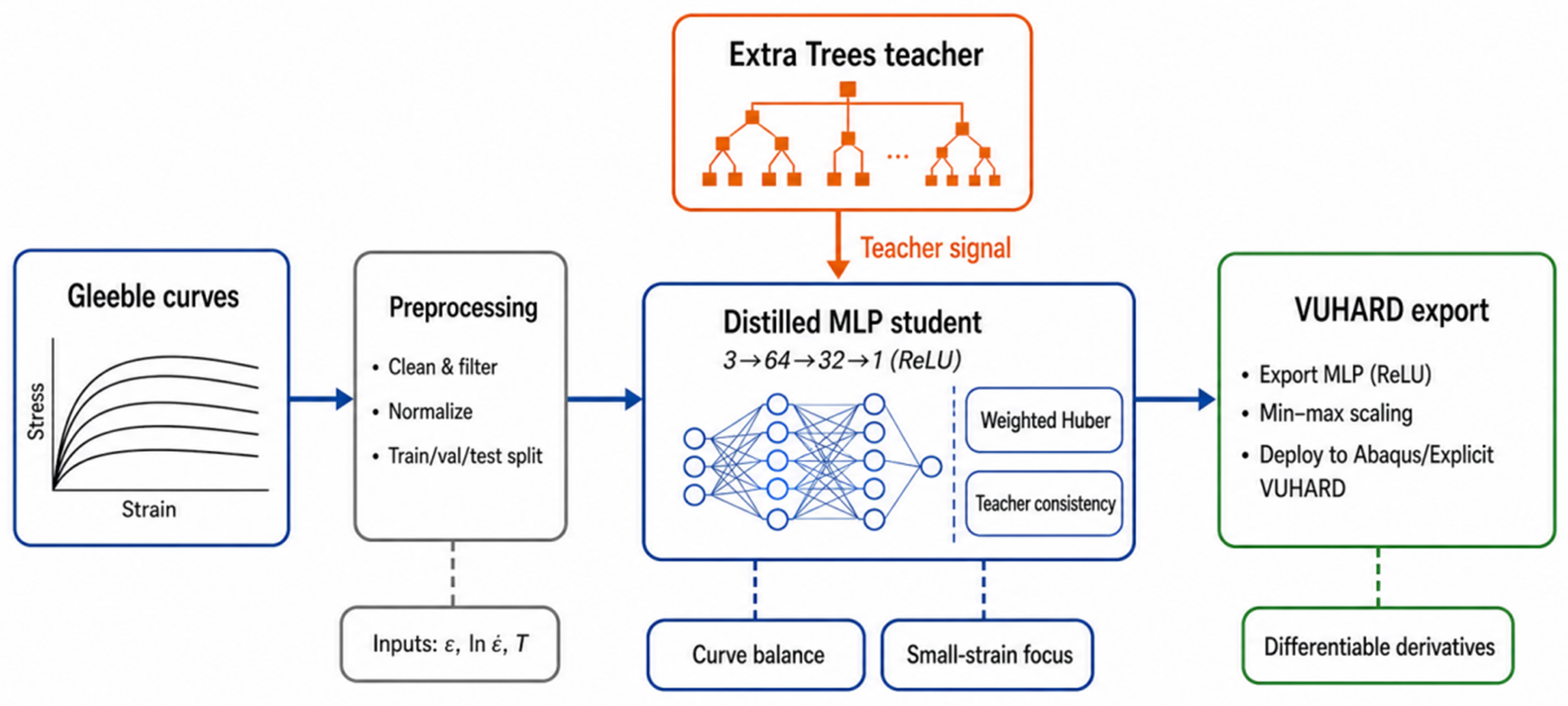
Figure 3. Schematic architecture of the KD-ANN model. KD-ANN: Knowledge-distilled artificial neural network; MLP: multilayer perceptron; ReLU: rectified linear unit.
We use a curve-grouped leave-one-temperature-out validation strategy to evaluate the ability of KD-ANN to predict flow behavior at previously unseen deformation temperatures. The dataset contains 24 complete flow-stress curves obtained at six temperatures (800, 850, 900, 950, 1,000 and 1,050 °C), with four strain rates examined at each temperature. A complete flow-stress curve, defined by a unique temperature–strain-rate combination, serves as the minimum unit for data partitioning. All strain–stress observations from the same curve are therefore assigned to a single data subset, preventing correlated neighboring points from appearing in both the training and test sets.
For each data point, the model input features are defined as follows:
X i = [εi, ln
The validation procedure comprises six folds, with each temperature used once as the held-out test condition. In each fold, all four curves measured at the target temperature are reserved as an independent test set. The remaining 20 complete curves, corresponding to the other five temperatures, are further partitioned at the curve level into 16 training curves and 4 validation curves. No complete curve contributes observations to more than one subset.
KD-ANN is reinitialized and trained independently in each fold, resulting in six separately trained models. In each fold, 16 complete curves are used for parameter estimation, while four additional curves are used for internal validation and hyperparameter selection. The four curves at the held-out temperature are used exclusively for testing and do not participate in parameter estimation, model validation or teacher-target generation. The teacher-algorithm type was determined through preliminary screening using the complete experimental dataset, as described in Section “Teacher–student model and knowledge distillation”. After Extra Trees was selected, both the teacher and student models were reinitialized and independently trained within each leave-one-temperature-out fold.
The natural logarithm of strain rate ln
Teacher–student model and knowledge distillation
Introducing a teacher model is not merely an additional predictive module; instead, it constructs supervision signals with richer feature information to enhance the student model’s capacity to characterize and fit complex rheological behaviors during hot compression. Conventional MLPs only adopt discrete experimentally measured flow stresses as training labels, with the optimization objective restricted to minimizing the global prediction error. Consequently, such models tend to prioritize fitting data regions with abundant samples and mild stress evolution, while failing to accurately capture intense work hardening at low strains, local abrupt variations near peak stress, and subtle curvature changes of stress curves in the dynamic softening stage.
To address this limitation, a knowledge distillation strategy is adopted in this work to establish a dual-model framework consisting of a teacher model and a student neural network. Specifically, a high-precision machine learning model with excellent predictive performance is selected as the teacher to extract implicit local rheological features hidden in experimental data and output soft supervision labels. A compact MLP is used as the student model to learn jointly from experimental stress values and teacher predictions, combining stress-prediction accuracy with a continuous constitutive representation suitable for FE implementation.
The teacher model is expected to generate high-accuracy soft targets that preserve the local variations in the experimental flow-stress response. To identify a suitable teacher algorithm and examine the basic student-network configuration, a preliminary model-screening experiment was conducted using the full experimental dataset. All experimental data points were randomly divided into an 80% training subset and a 20% test subset, and all candidate models were evaluated using the same data partition. The root mean square error (RMSE) is used as the principal criterion for teacher-model selection and is defined as:
The results presented in Figure 4 show that Extra Trees yields the lowest prediction error among the candidate machine-learning algorithms and is therefore selected as the teacher algorithm for the subsequent knowledge-distillation framework. The Extra Trees model trained during this preliminary comparison is used solely to identify the teacher algorithm and is not carried forward into the leave-one-temperature-out evaluation. Once the teacher algorithm is determined, its model parameters are reinitialized in each validation fold, and a new Extra Trees model is trained exclusively on the corresponding training subset. The resulting predictions at the original training coordinates are then used as soft targets for the student network. Thus, neither the fitted teacher model nor information from the held-out temperature is transferred to the training process of the corresponding fold. It should also be noted that the results in Figure 4 are used only for preliminary algorithm and network-configuration screening and do not represent the final generalization performance of KD-ANN. Therefore, the RMSE values shown in Figure 4 should not be directly compared with the leave-one-temperature-out metrics reported in the subsequent sections.
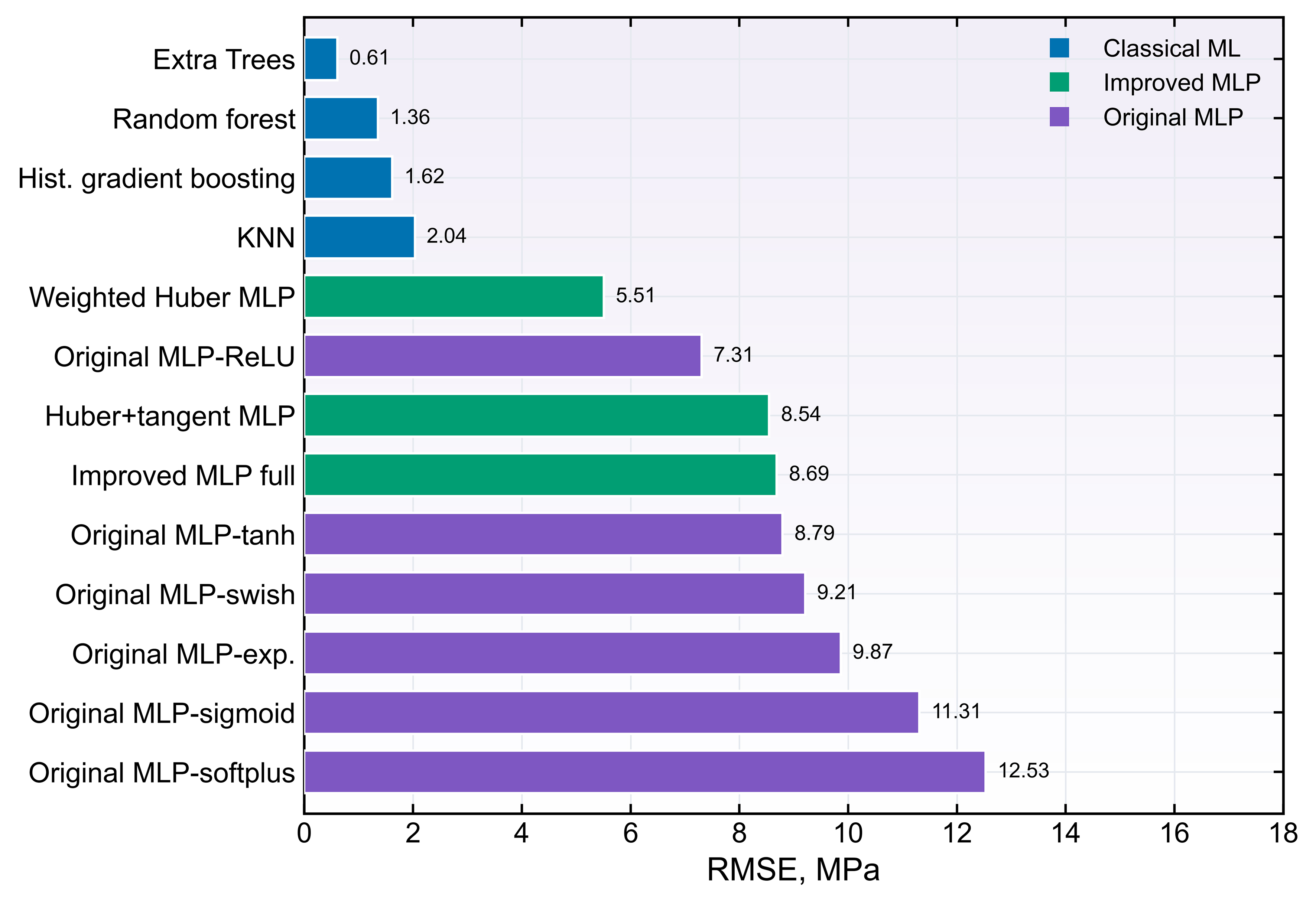
Figure 4. Preliminary performance comparison of candidate teacher algorithms and student-network configurations using an 80/20 pointwise split of the complete dataset. These results are used only for model screening and do not represent the final leave-one-temperature-out generalization performance. KNN: K-nearest neighbors; MLP: multilayer perceptron; ReLU: rectified linear unit; ML: machine learning; RMSE: root mean square error.
Nevertheless, because the preliminary screening employed an 80/20 pointwise split of the complete dataset, the teacher-algorithm and basic student-architecture choices were informed by data from all six temperatures. These choices were therefore not made completely independently of the subsequently held-out temperature data. Although the teacher and student models are newly fitted within each leave-one-temperature-out fold, the preliminary selection procedure may introduce some model-selection optimism. Consequently, the leave-one-temperature-out results evaluate the out-of-sample performance of the selected modeling configuration rather than providing a fully independent evaluation of the entire algorithm- and architecture-selection process. The preliminary screening results in Figure 4 and the subsequent temperature-wise validation results therefore serve different purposes and are interpreted separately.
Despite its high predictive accuracy, Extra Trees is a tree-based ensemble algorithm that produces piecewise-constant prediction functions without global continuous differentiability. It therefore cannot be expressed directly as an explicit differentiable constitutive equation or readily integrated into FE material subroutines. Consequently, Extra Trees is used exclusively as the teacher model in the knowledge-distillation framework rather than as the final constitutive model. The prediction output of the teacher model for an arbitrary input sample xi is defined as:
where FET denotes the trained Extra Trees teacher model, and σiT represents the soft label output by the teacher model.
A feedforward fully connected MLP with rectified linear unit (ReLU) hidden-layer activations and a linear output layer is selected as the student model. The network defines a continuous, piecewise-affine mapping in the normalized input space and is differentiable almost everywhere, allowing its forward calculation and derivative evaluation to be exported to Fortran. This MLP is established to characterize the nonlinear mapping between hot deformation parameters and flow stress, which is formulated as follows:
where θ denotes all trainable network parameters. The student network adopts a 3–64–32–1 topology, consisting of an input layer with three neurons, two hidden layers containing 64 and 32 neurons, respectively, and a single-neuron output layer for predicting flow stress. Including weights and biases, the student network contains 2,369 trainable parameters. Its forward propagation process is expressed as:
where
In Equation (9), ϕ denotes the ReLU activation, ϕ(z) = max(0, z). Its derivative is 1 for z > 0 and 0 for z < 0; at z = 0, a slope of zero is assigned as a numerical convention. The same convention is used in the exported VUHARD implementation. Stress derivatives are evaluated by the chain rule, accounting for input normalization, the logarithmic strain-rate transformation, and output rescaling.
Considering the uneven number of data points contained in different flow curves, a curve balance weight (wicurve) is introduced in this work to prevent curves with more sampling points from dominating the training process. Meanwhile, the low-strain region corresponds to the critical deformation stage at the initial forming period and exerts a remarkable influence on the subsequent load–displacement response. Accordingly, a low-strain enhancement weight is further proposed:
where wi is the final weight assigned to the i-th training sample, wicurve denotes the curve-balancing weight used to prevent curves containing more data points from dominating the training process, and εi is the true strain corresponding to the i-th sample. The parameter β controls the magnitude of the additional weighting in the low-strain region, while τ controls the rate at which this enhancement decays with increasing strain. At εi = 0, the enhancement factor reaches its maximum value of 1 + β; as strain increases, the exponential term gradually approaches zero and wi approaches wicurve.
To improve robustness against local experimental fluctuations and samples with relatively large residuals, the Huber loss is used for supervision based on the experimental stresses. The Huber loss combines the characteristics of the mean squared error and mean absolute error. For small residuals, it adopts a quadratic form to provide smooth gradients and accurate fitting. For large residuals, it changes to a linear form to reduce sensitivity to outliers. For the residual:
the Huber loss is defined as:
where δ is the transition threshold between the quadratic and linear regions. A smaller value of δ increases robustness to large residuals, whereas a larger value makes the loss behave more similarly to the mean squared error. The weighted Huber loss for supervision using the experimental ground-truth stresses is expressed as:
whereas the weighted consistency loss between the student-network predictions and teacher-generated targets is defined as:
The final knowledge-distillation objective is then formulated as:
here,
After training, the input and output normalization parameters were exported together with the network weights and biases for implementation in the Fortran VUHARD subroutine.
Prediction accuracy: modified J–C model vs. KD-ANN model
To ensure a fair comparison with the KD-ANN model, the modified J–C model is evaluated using exactly the same curve-grouped leave-one-temperature-out protocol. In each fold, all four flow-stress curves at one deformation temperature are retained as the common independent test set, whereas only the curves obtained at the remaining five temperatures are used for parameter identification. The modified J–C model is recalibrated independently in each fold, and no data point from the held-out temperature is involved in the fitting procedure. The parameter-identification procedure follows that described in Ref.[8]. The resulting fold-specific constitutive equations for the independently held-out temperatures of 800, 850, 900, 950, 1,000 and 1,050 °C are given in Equations (16)-(21), respectively.
σ = (102.22 - 134.98ε + 108.49ε2)(1.12 + 0.57 ln
σ = (135.91 - 121.78ε + 77.82ε2)(1 + 0.44ln
σ = (135.91 - 121.78ε + 77.82ε2)(1 + 0.44ln
σ = (135.91 - 121.78ε + 77.82ε2)(1 + 0.44ln
σ = (135.91 - 121.78ε + 77.82ε2)(1 + 0.44ln
σ = (135.91 - 121.78ε + 77.82ε2)(1 + 0.44ln
here,
To quantitatively assess the predictive performance of the developed models, the coefficient of determination (R2) and mean absolute error (MAE) are adopted as evaluation metrics, together with the aforementioned RMSE[34-36]. The definitions of these indicators are given as follows:
Figure 5 compares the experimental and predicted stresses obtained using the modified J–C model under curve-grouped leave-one-temperature-out validation. Averaged across the six held-out temperature folds, the model achieves an R2 of 0.960, an RMSE of 17.12 MPa and an MAE of 12.58 MPa. The predictions capture the overall flow-stress response of complete curves at unseen temperatures, although accuracy varies among folds. The largest RMSE and MAE occur at 800 °C, while the lowest R2 is observed at 1,050 °C. Overall, the modified J–C model reproduces the general stress response of the complete flow curves at unseen temperatures, although its predictive accuracy varies among the held-out temperature conditions.
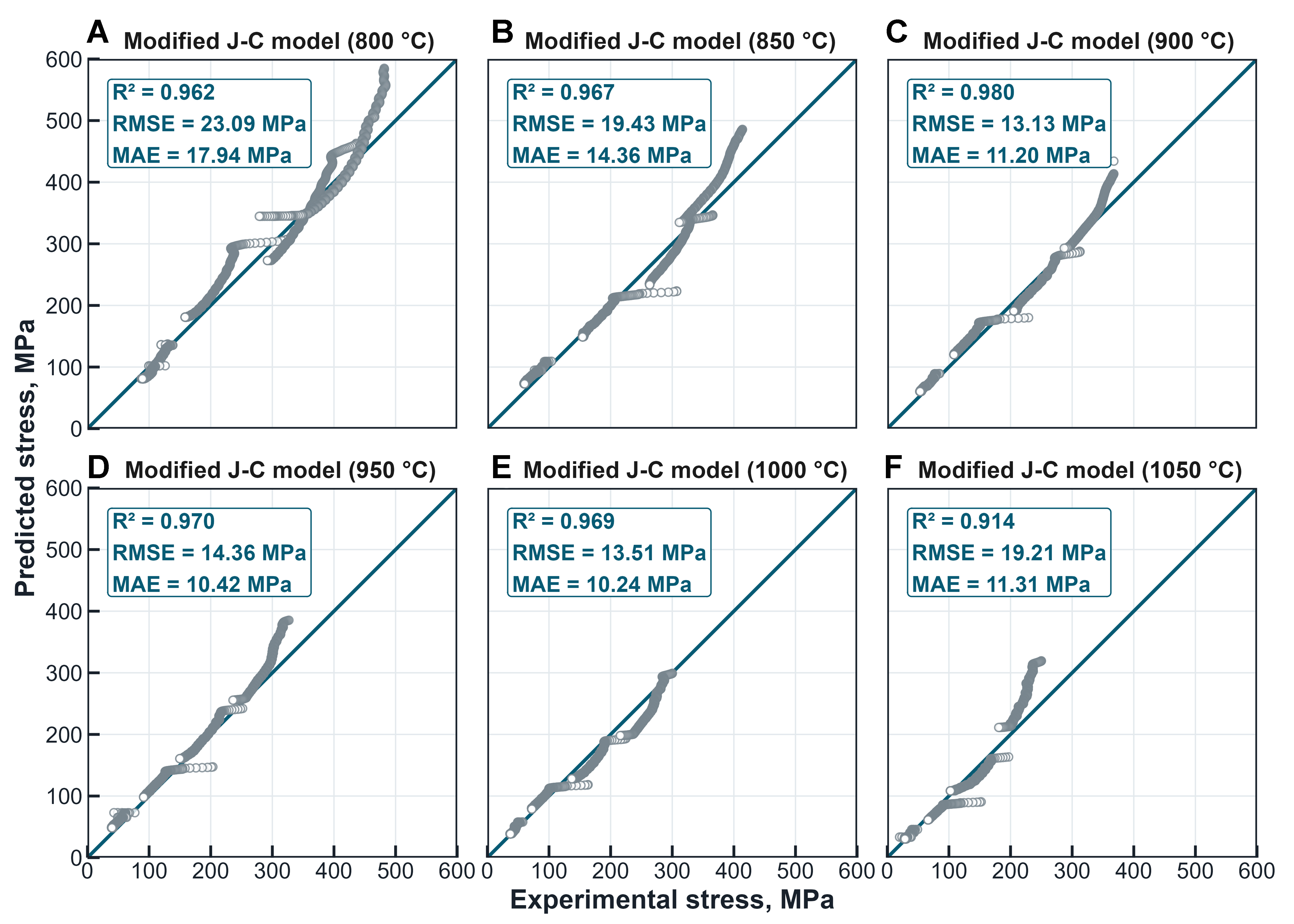
Figure 5. Predictive performance of the modified J–C model across different held-out temperatures: (A) 800 °C, (B) 850 °C, (C) 900 °C, (D) 950 °C, (E) 1,000 °C, (F) 1,050 °C. J–C: Johnson–Cook; R2: coefficient of determination; RMSE: root mean square error; MAE: mean asbsolute error.
Figure 6 shows the predictions of KD-ANN under leave-one-temperature-out validation. In each validation fold, all four flow curves at the target temperature are excluded from training and validation and are used exclusively for testing. KD-ANN achieves R2 values of 0.978-0.991, RMSE values of 7.57-14.83 MPa and MAE values of 5.79-12.21 MPa. Averaged across the six held-out temperatures, R2, RMSE and MAE reach approximately 0.984, 11.40 and 9.21 MPa, respectively. The highest R2 is obtained at 900 °C (R2 = 0.991), whereas the lowest RMSE and MAE are achieved at 1,050 °C (7.57 and 5.79 MPa, respectively). Even at the lower boundary of 800 °C, KD-ANN maintains an c of 0.985, with RMSE and MAE values of 14.46 and
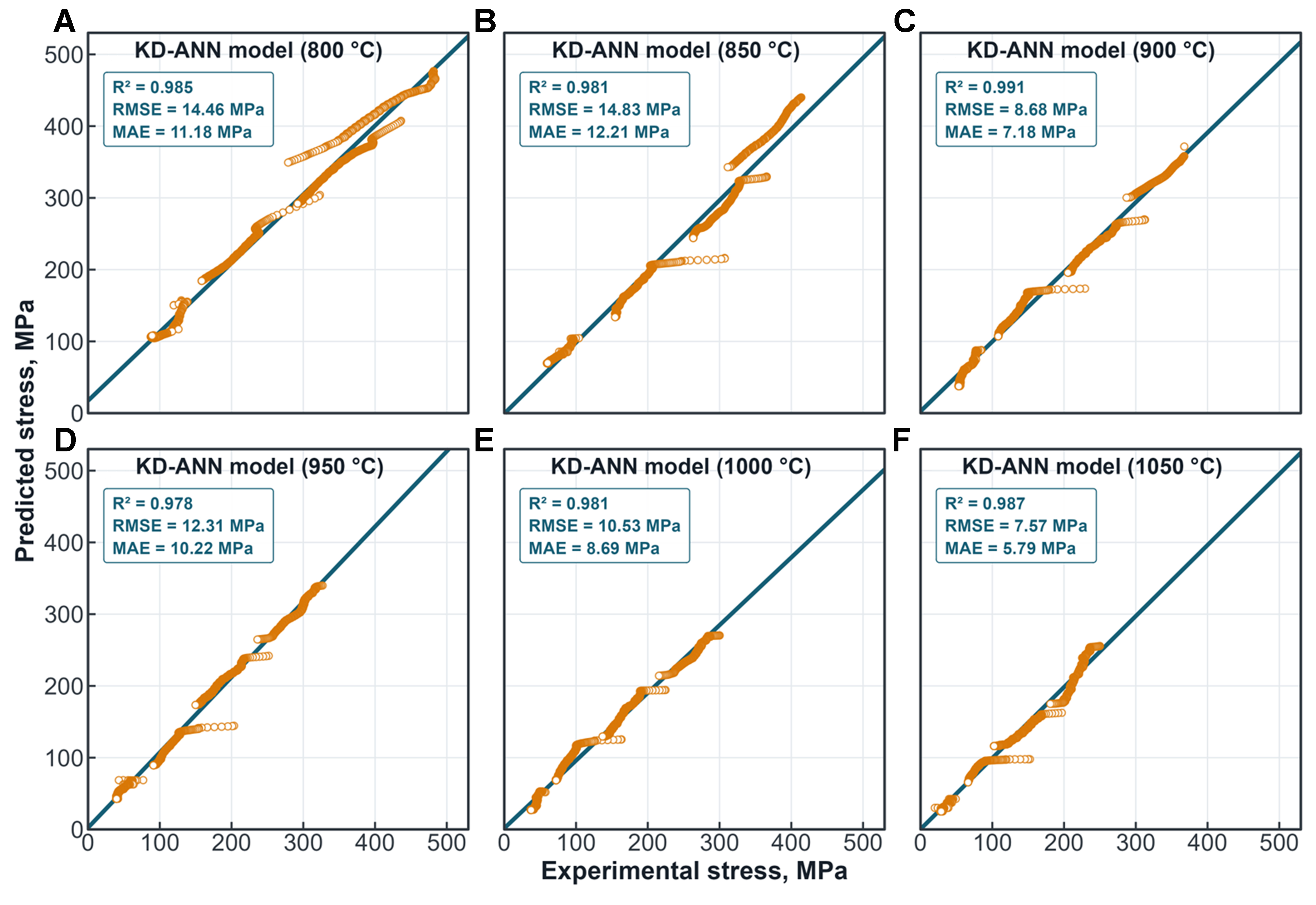
Figure 6. Predictive performance of the KD-ANN model across different held-out temperatures: (A) 800 °C, (B) 850 °C, (C) 900 °C, (D) 950 °C, (E) 1,000 °C, (F) 1,050 °C. KD-ANN: Knowledge-distilled artificial neural network; R2: coefficient of determination; RMSE: root mean square error; MAE: mean absolute error.
The relative gains shown in Figure 7 further quantify the predictive advantage of KD-ANN under the unified leave-one-temperature-out protocol. Positive gains are obtained for all three metrics at each investigated temperature. On average, KD-ANN increases R2 by 23.3 × 10-3 and reduces RMSE and MAE by 32.0% and 25.7%, respectively. The largest improvements occur at 1,050 °C, where R2 increases by 72.8 × 10⁻³, while RMSE and MAE decrease by 60.6% and 48.8%, respectively. At 950 °C, the MAE reduction is relatively modest at 1.9%. Nevertheless, KD-ANN still increases R2 by 7.9 × 10-3 and reduces RMSE by 14.3% under this condition.
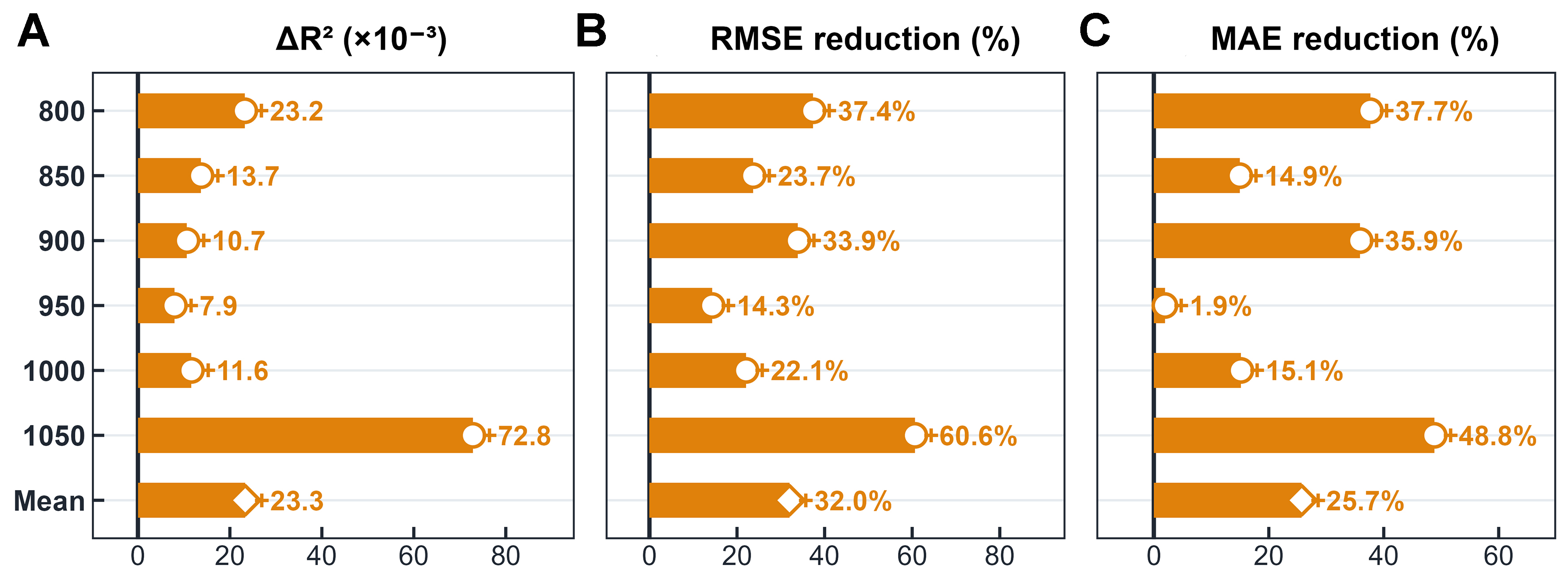
Figure 7. Predictive performance gains of KD-ANN over the J–C model at different held-out temperatures. KD-ANN: Knowledge-distilled artificial neural network; J–C: Johnson–Cook; R2: coefficient of determination; RMSE: root mean square error; MAE: mean absolute error.
The improvements at 800 and 1,050 °C are particularly relevant because these temperatures represent the lower and upper boundaries of the investigated domain. At 800 °C, KD-ANN increases R2 by 23.2 × 10-3 and reduces RMSE and MAE by 37.4% and 37.7%, respectively. At 1,050 °C, the corresponding reductions reach 60.6% and 48.8%. The consistent gains at both intermediate and boundary temperatures indicate that KD-ANN captures transferable relationships among strain, strain rate, temperature and flow stress. These results support its generalization to complete deformation curves at unseen temperatures and its short-range extrapolation at the boundaries of the investigated temperature range.
Notably, both KD-ANN and the modified J–C model are evaluated using the same curve-grouped leave-one-temperature-out protocol. In each fold, both models are developed exclusively from the five retained temperatures and then used to predict the complete flow-stress curves at the held-out temperature. Under this identical evaluation setting, KD-ANN achieves higher R2 values and lower RMSE and MAE values across all six temperatures. Its consistent advantage at both intermediate and boundary temperatures indicates a stronger ability to capture the nonlinear relationships among strain, strain rate, temperature and flow stress. Overall, these results demonstrate that KD-ANN provides greater predictive accuracy and transferability than the modified J–C model under previously unseen temperature conditions.
Additional leave-one-strain-rate-out validation is conducted to assess generalization along the strain-rate dimension [Supplementary Material 1]. Predictive accuracy decreased when an entire strain-rate condition was excluded, particularly near the boundaries of the investigated range. This weaker performance is likely associated with the limited experimental sampling along the strain-rate dimension. Thus, the favorable temperature-wise results should not be interpreted as equally strong generalization to unseen strain rates. Future work will include more closely spaced strain-rate conditions to improve and reassess this capability.
Ablation analysis of the KD-ANN framework
To evaluate the incremental effects of the components used in the proposed KD-ANN framework, a sequential ablation study was conducted under the same curve-grouped leave-one-temperature-out validation protocol. All configurations used the same 3–64–32–1 MLP architecture and identical curve partitions. Therefore, the comparisons concern differences in the training objectives and weighting strategies rather than changes in network depth or width. The reported metrics are the arithmetic means of the corresponding results obtained from the six held-out-temperature folds.
Four configurations were considered in the sequential ablation. The original MLP was trained using the conventional MSE objective without curve-balancing or low-strain weighting. The weighted MLP retained the MSE objective but introduced curve-balancing and low-strain weights. KD-ANN without teacher supervision replaced the MSE objective with the weighted Huber loss while retaining both weighting strategies. The complete KD-ANN further incorporated the teacher-target consistency loss. The components included in each configuration are summarized in Table 2.
Configurations and results of the sequential ablation study under curve-grouped leave-one-temperature-out validation
| Model | Experimental-label loss | Curve balancing | Low-strain weighting | Teacher-target loss | RMSE (MPa) | MAE (MPa) | R2 |
| Original MLP | MSE | No | No | No | 22.37 | 19.17 | 0.932 |
| Weighted MLP | MSE | Yes | Yes | No | 21.12 | 16.66 | 0.942 |
| KD-ANN without teacher | Weighted Huber | Yes | Yes | No | 17.87 | 14.39 | 0.958 |
| Complete KD-ANN | Weighted Huber | Yes | Yes | Weighted teacher-target MSE | 11.40 | 9.21 | 0.984 |
The original MLP achieved an RMSE of 22.37 MPa, an MAE of 19.17 MPa and an R2 of 0.932. Introducing the curve-balancing and low-strain weighting strategies reduced the RMSE and MAE to 21.12 and
KD-ANN without teacher supervision achieved an RMSE of 17.87 MPa, an MAE of 14.39 MPa and an R2 of 0.958. Relative to the weighted MLP, the RMSE and MAE decreased by 15.4% and 13.6%, respectively. The complete KD-ANN achieved the lowest errors, with an RMSE of 11.40 MPa, an MAE of 9.21 MPa and an R2 of 0.984. Compared with KD-ANN without teacher supervision, the complete model reduced RMSE and MAE by 36.2% and 36.0%, respectively. Relative to the original MLP, the corresponding reductions were 49.0% and 52.0%.
Because the components were introduced sequentially, the observed increments depend on the components already included in the preceding configuration. The sequential ablation therefore supports the progressive construction of the complete framework but does not provide an order-independent decomposition of the contribution of each component.
To examine teacher supervision more directly, additional targeted control experiments were conducted using the same student architecture, curve partitions, weighting strategies and validation procedure. In each fold, the Extra Trees teacher was trained exclusively using the 16 training curves, and its predictions at the original training coordinates were used as soft targets. The validation and held-out test curves were not used to fit the teacher, generate training targets or update the student-model parameters.
Let H(y) denote the weighted Huber loss between the student prediction and the measured stress y, and let M(Z) denote the weighted MSE between the student prediction and target z. Four matched student configurations were compared. Configuration A used only the experimental-label Huber loss. Configuration B was trained exclusively against the teacher-generated targets. Configuration C represented the complete KD-ANN and combined experimental and teacher supervision. Configuration D retained the same mixed-loss structure and weighting coefficients as Configuration C but replaced the teacher targets with measured stresses. The training objectives and purposes of these configurations are summarized in Table 3.
Training objectives and purposes of the model configurations used in the teacher-supervision control experiments
| Configuration | Training objective | Purpose |
| Conventional MLP | Conventional experimental-label training | Baseline MLP performance |
| A: No-teacher KD student | H(y) | Performance without auxiliary teacher supervision |
| B: Teacher-only pseudo-label MLP | M(yT) | Performance when the student is trained exclusively using teacher predictions |
| C: Complete KD-ANN | 0.65H(y) + 0.35M(yT) | Performance under joint experimental and teacher supervision |
| D: Experimental-target control | 0.65H(y) + 0.35M(y) | Effect of using the same mixed-loss structure without teacher-generated targets |
Here, yT denotes the prediction generated by the fold-specific Extra Trees teacher. Configuration B is an MLP student trained against teacher-generated pseudo-labels rather than the Extra Trees model itself. Configuration D controls for the effect of introducing an additional MSE term without using teacher-generated targets.
The predictive performance of the control configurations is summarized in Table 4. All reported values are the arithmetic means across the six held-out-temperature folds.
Predictive performance of the teacher-supervision control configurations under curve-grouped leave-one-temperature-out validation
| Configuration | RMSE (MPa) | MAE (MPa) | R2 |
| Conventional MLP | 22.37 | 19.17 | 0.932 |
| A: No-teacher KD student | 17.87 | 14.39 | 0.958 |
| B: Teacher-only pseudo-label MLP | 16.03 | 11.87 | 0.966 |
| C: Complete KD-ANN | 11.40 | 9.21 | 0.984 |
| D: Experimental-target control | 22.84 | 20.25 | 0.935 |
The teacher-only pseudo-label MLP improved upon both the conventional MLP and the no-teacher KD student, indicating that the teacher predictions provide a useful supervisory signal. However, teacher-only training did not reproduce the performance of the complete KD-ANN. Compared with Configuration B, Configuration C reduced RMSE and MAE by approximately 28.9% and 22.4%, respectively. This comparison indicates that joint supervision using experimental stresses and teacher-generated targets is more effective than exclusive imitation of the teacher.
Configuration D achieved an RMSE of 22.84 MPa, an MAE of 20.25 MPa and an R2 of 0.935. Under the same mixed-loss structure, replacing the auxiliary experimental target with the teacher-generated target reduced RMSE and MAE by approximately 50.1% and 54.5%, respectively. The comparison between Configurations C and D therefore supports an additional predictive benefit from using teacher-generated targets within the joint-supervision objective.
The teacher targets are generated only at the original training coordinates and introduce no additional experimental observations or deformation conditions. Although the results demonstrate the predictive benefit of the complete teacher-supervised configuration, they do not fully distinguish genuine knowledge transfer from possible smoothing, pseudo-label or loss-interaction effects. Accordingly, the present results are interpreted as evidence supporting the practical value of the joint training formulation rather than proof of a unique underlying mechanism. Further controlled experiments and additional hot-compression data will be used in future work to examine these effects separately.
Overall, the sequential ablation and targeted control experiments show that the performance of KD-ANN arises from the combined effects of its training components. The weighting and Huber-based student-training strategies provide progressive improvements over the original MLP, while the joint use of experimental stresses and teacher-generated targets produces the largest incremental gain under the present validation protocol.
Although validation-based early stopping, checkpoint selection and complete-curve holdout mitigate the risk of overfitting, they cannot demonstrate its complete absence. The present dataset contains only 24 distinct temperature–strain-rate conditions, and observations along each flow curve are correlated rather than independent experimental replicates. Therefore, the present validation supports the temperature-wise predictive capability of the selected model configuration but does not establish unrestricted generalization beyond the sampled thermomechanical domain. The validated application range is limited to temperatures of 800-1,050 °C, strain rates of 0.01-10 s-1, and the investigated strain range. Predictions outside these ranges should be treated cautiously until additional independent experimental data become available.
Comparative FE simulation of J–C and KD-ANN constitutive models
Since the data measured by the Gleeble system is typically obtained under the assumptions of negligible interfacial friction and no temperature gradient, the FE model in this study was also established under idealized hot-compression conditions to verify the applicability of the proposed machine learning-based constitutive model. Specifically, the specimen–anvil contact was treated as approximately frictionless, and the temperature field within the specimen was assumed to remain spatially uniform, so that the constitutive response could be evaluated under idealized hot-compression conditions. The reaction force–displacement curve obtained from the FE simulation was then compared with the rheological response output by the Gleeble system. If the two curves show consistent profiles and similar evolution trends, it indicates that the proposed machine learning constitutive model can provide reliable predictions under idealized conditions and is therefore feasible and applicable for FE simulations.
For the FE validation at 800 °C, the fold-specific KD-ANN student model obtained from the leave-one-temperature-out fold in which 800 °C served as the held-out test temperature was employed. In this fold, all four flow-stress curves measured at 800 °C were excluded from teacher and student training and validation and were used exclusively for independent testing. The FE model of isothermal hot compression is shown in Figure 8, where Figure 8A presents the schematic diagram of the isothermal hot compression model and Figure 8B shows the geometric meshing of the model. Following the method proposed by Pantalé et al.[30], the corresponding KD-ANN student model was implemented in Abaqus/Explicit through the VUHARD user subroutine to simulate the isothermal compression process at all four experimental strain rates. For comparison, the modified J–C model was also incorporated into the same FE framework, while all other geometric, contact, meshing, and boundary conditions were kept identical. The dies were modeled as rigid bodies, whereas the specimen was defined as a deformable body with an initial temperature of 800 °C. Because the simulation was conducted under idealized isothermal hot-compression conditions, no heat transfer coefficient was applied between the specimen and the anvils. A small friction coefficient of 0.01 was introduced at the specimen–anvil interface solely to improve numerical stability and avoid severe mesh distortion and non-convergence that may occur under a strictly frictionless condition. Owing to its very small magnitude, the associated frictional effect was considered negligible, and the contact condition was therefore regarded as approximately frictionless. The specimen was discretized using C3D8RT hexahedral elements with a mesh size of 0.5 mm.
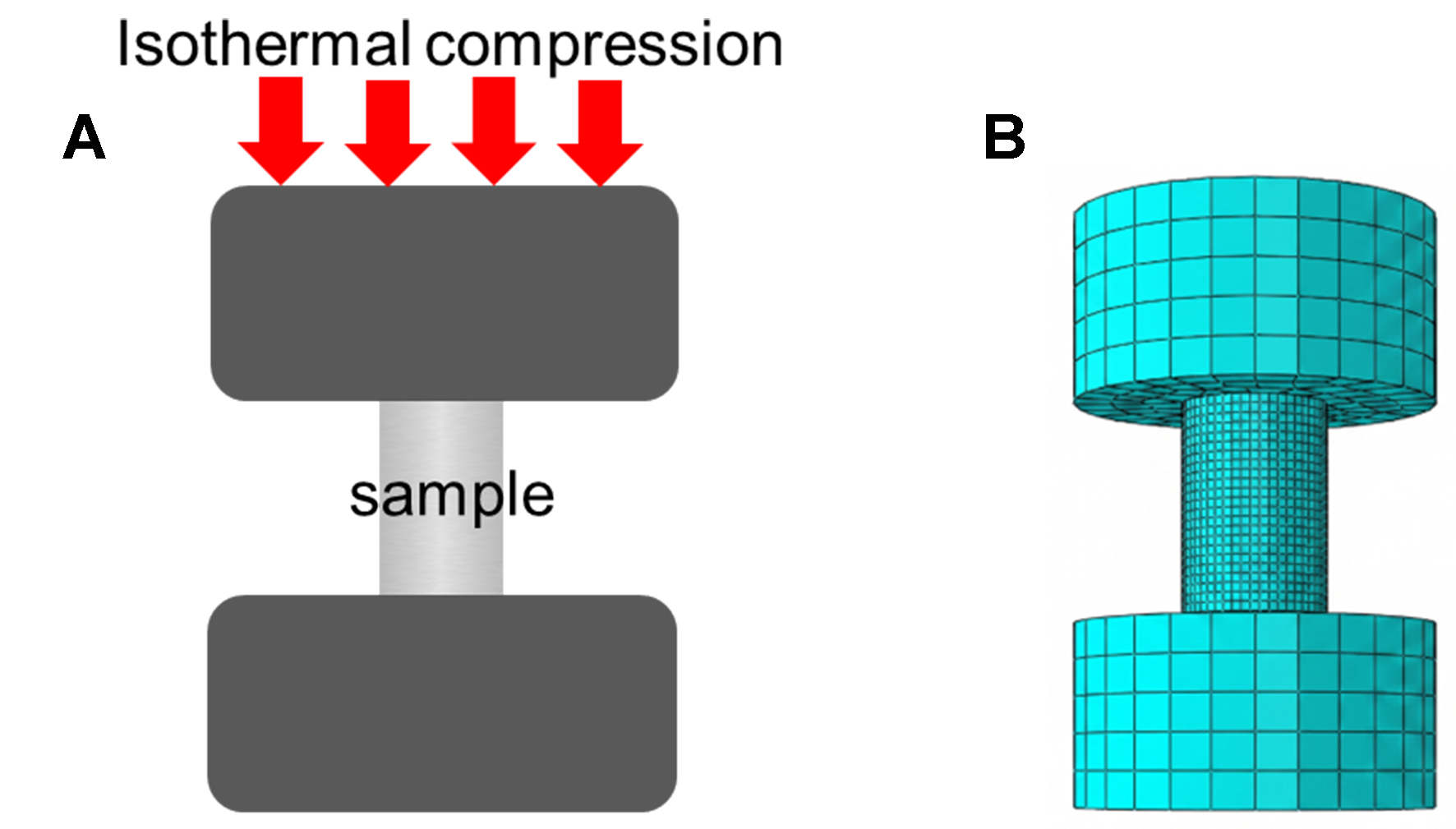
Figure 8. (A) Schematic diagram of the isothermal hot compression model; (B) FE meshing of the model. FE: Finite element.
The contour maps of equivalent strain and equivalent stress obtained from FE simulations are presented in Figures 9 and 10, respectively. It can be seen that, under the same deformation temperature and strain rate, the overall deformation characteristics predicted by the KD-ANN constitutive model and the J–C constitutive model are highly consistent when used as material inputs in the FE analysis. The equivalent strain predicted by both models is mainly concentrated in the central region of the specimen, exhibiting a distinct layered distribution along the height direction, whereas the equivalent strain near the upper and lower end faces is relatively small. This is mainly because the heat transfer between the specimen and the anvils is not considered in the present simulation, and the friction coefficient is set to a low value, resulting in a relatively weak constraint at the end faces. As a result, the overall deformation of the specimen is more uniform, and no pronounced barreling is observed.
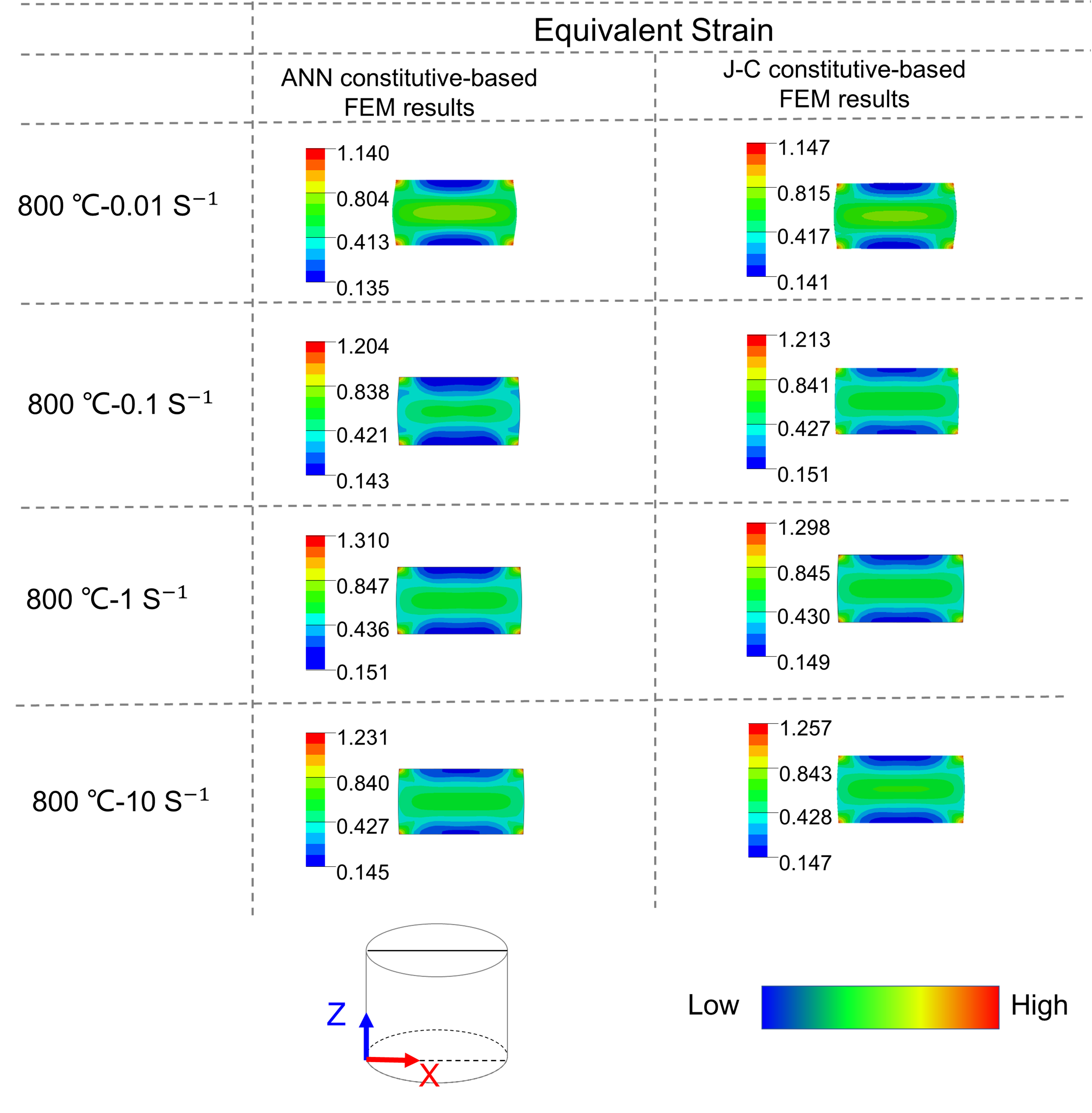
Figure 9. Distribution of equivalent strain from ideal compression FE simulations predicted by the KD-ANN and J–C constitutive models. FE: Finite element; KD-ANN: knowledge-distilled artificial neural network; J–C: Johnson–Cook; FEM: finite element method.
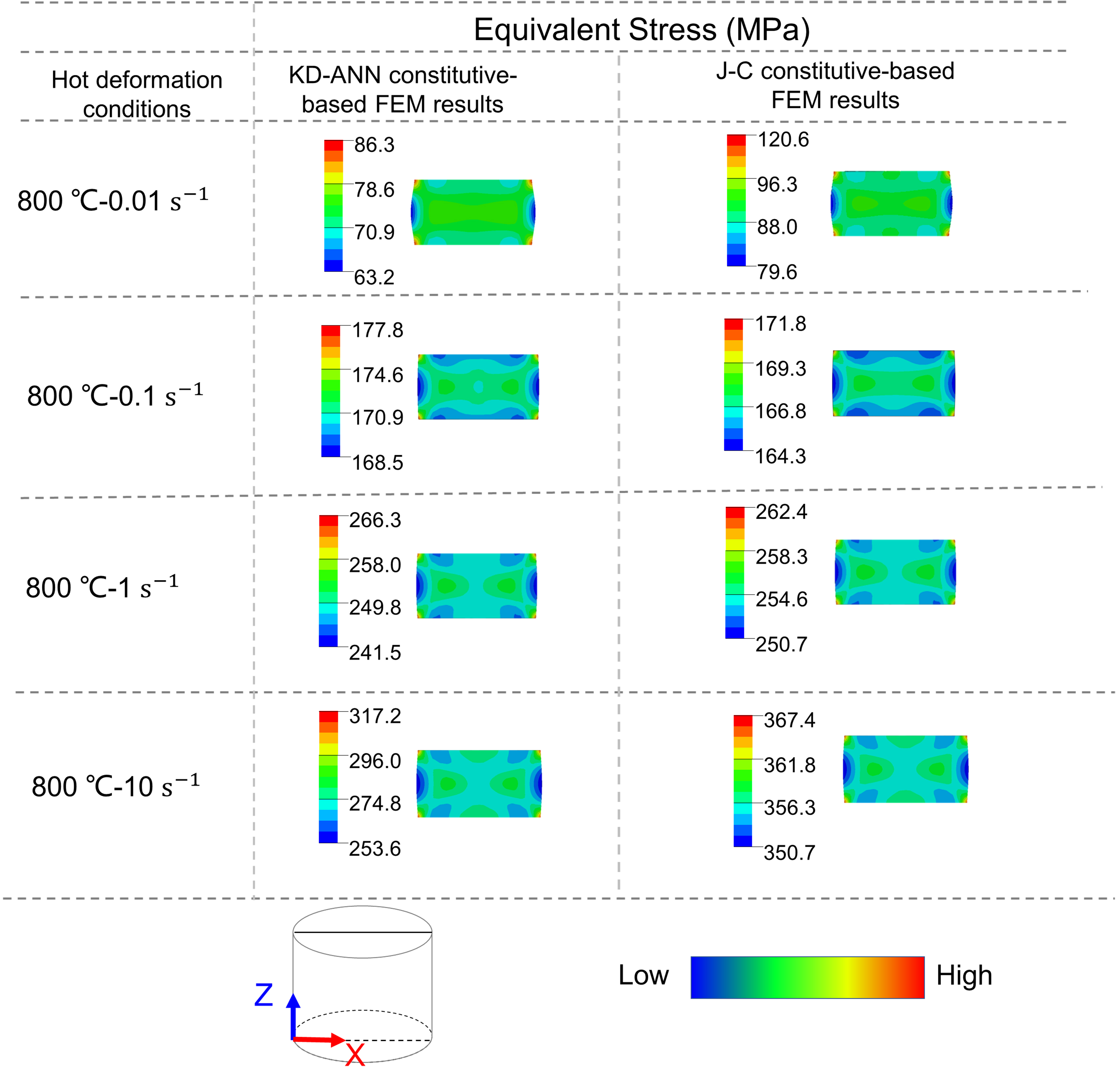
Figure 10. Distribution of equivalent stress from ideal compression FE simulations predicted by the KD-ANN and J–C constitutive models. FE: Finite element; KD-ANN: knowledge-distilled artificial neural network; J–C: Johnson–Cook; FEM: finite element method.
Further comparison of the equivalent stress distribution shows that the stress fields predicted by the two constitutive models exhibit essentially the same distribution pattern: the equivalent stress is relatively low in the end regions of the specimen, whereas the central region and its vicinity show a higher stress level, indicating that the load during plastic deformation is mainly concentrated within the specimen interior. As the strain rate increases, the equivalent stress inside the specimen shows an overall upward trend, suggesting that the material exhibits a certain degree of strain-rate sensitivity under high strain-rate conditions. Overall, both the ANN constitutive model and the J–C constitutive model are able to capture the macroscopic deformation behavior of the specimen and the distribution characteristics of the flow field during hot compression.
Figure 11 compares the experimentally measured load–displacement curves with the FE predictions obtained using the modified J–C and KD-ANN constitutive models at 800 °C. Both models reproduce the overall evolution of the experimental load, including its rapid increase during the initial loading stage and subsequent variation with displacement. Nevertheless, the KD-ANN-based simulations show closer agreement with the experimental curves across the four strain rates. At 0.01, 0.1, 1 and 10 s-1, the MAEs obtained using KD-ANN are 0.293, 0.238, 0.698 and 1.686 kN, respectively, whereas those obtained using the modified J–C model are 0.513, 1.014, 1.608 and 1.716 kN, respectively. The corresponding mean MAEs over the four deformation conditions are 0.729 kN for KD-ANN and 1.213 kN for the modified J–C model. These results demonstrate that the KD-ANN constitutive model provides a more accurate description of the experimentally observed load response over the investigated range of strain rates.
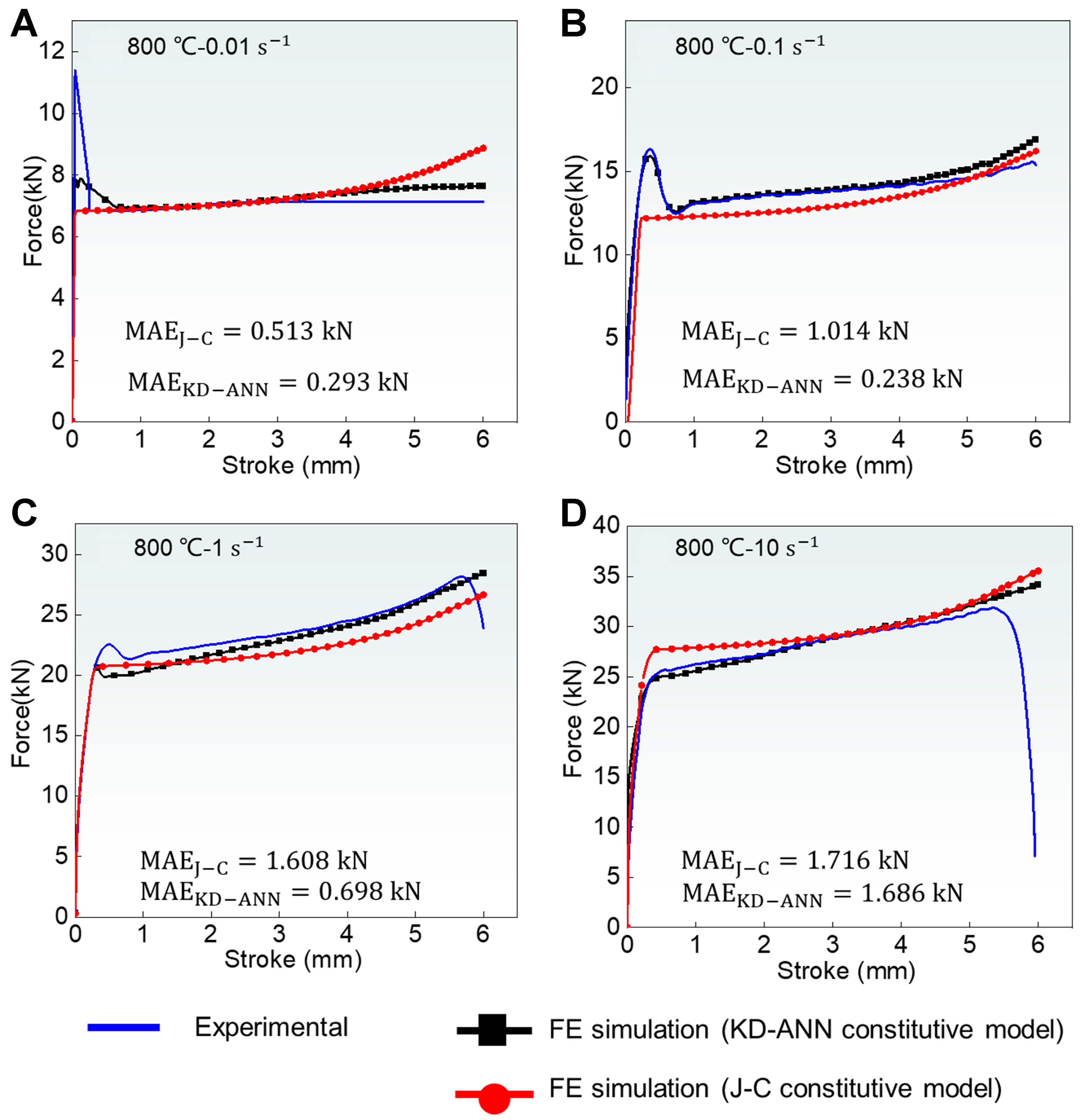
Figure 11. Comparisons of the forming load of the predicted values by KD-ANN constitutive model and the modified J–C constitutive model. KD-ANN: Knowledge-distilled artificial neural network; J–C: Johnson–Cook; MAE: mean absolute error.
The improvement is particularly pronounced at strain rates of 0.1 and 1 s-1, where KD-ANN more accurately captures the experimental load evolution throughout the principal deformation stage. At 10 s-1, the experimental load drops abruptly near the end of the test because the Gleeble servo-control system initiates rapid deceleration and unloading as the actuator approaches the prescribed displacement. This terminal decrease is therefore an equipment-control response rather than an intrinsic material response and cannot be reproduced by the constitutive model. The corresponding unloading data are excluded from the error evaluation, and the comparison is restricted to the effective loading stage. Within this range, the two models exhibit comparable errors, although KD-ANN still yields a slightly lower MAE. Overall, the close agreement between the KD-ANN-driven FE predictions and the experimental measurements confirms that the model can be successfully implemented in an Abaqus material subroutine and retains strong generalization capability when predicting structural responses at a deformation temperature entirely excluded from model development.
Combined with the equivalent strain and stress distributions, the load–displacement results show that both the KD-ANN and modified J–C constitutive models reproduce the overall macroscopic deformation characteristics of the specimen during hot compression. However, the KD-ANN-based simulations exhibit consistently closer agreement with the experimental load–displacement curves across the four strain rates. This improvement arises from the enhanced ability of KD-ANN to represent the nonlinear dependence of flow stress on strain, strain rate and temperature, thereby providing a more accurate prediction of the structural load response throughout the principal deformation stage and at large displacements.
Notably, all experimental curves at 800 °C are excluded from model training and validation. The agreement obtained at this completely unseen temperature therefore demonstrates not only the successful implementation of KD-ANN in Abaqus but also its extrapolation capability at the FE level. Compared with the modified J–C model, KD-ANN reduces the mean MAE of the predicted load from 1.213 to 0.729 kN. Further comparisons at the intermediate temperature of 900 °C and the upper-boundary temperature of 1,050 °C [Supplementary Material 2] show that KD-ANN generally retains closer agreement with the experimental load–displacement curves than the modified J–C model. These results demonstrate that KD-ANN provides a more accurate and reliable constitutive description for FE simulations of the high-temperature compression of the investigated alloy, supporting its application in hot-deformation prediction and process-parameter optimization.
CONCLUSIONS
A KD-ANN constitutive model is developed for the hot deformation of β-C titanium alloy. The main conclusions are as follows:
(1) Under the same curve-grouped leave-one-temperature-out validation protocol, KD-ANN achieves mean values of R2 = 0.984, RMSE = 11.40 MPa and MAE = 9.21 MPa, compared with 0.960, 17.12 MPa and 12.58 MPa, respectively, for the modified J–C model. This matched-fold comparison demonstrates that the selected KD-ANN configuration predicts complete flow-stress curves at held-out temperatures more accurately than the modified J–C model.
(2) The sequential ablation analysis shows that the weighting strategy and Huber-based student-training formulation progressively improve the baseline MLP. The targeted control experiments further show that the joint use of experimental stresses and teacher-generated targets produces the largest incremental improvement under the tested training protocol.
(3) For the fold in which all 800 °C curves are excluded from model fitting and validation, the KD-ANN-based FE simulations reproduce the experimental load–displacement curves with a mean MAE of 0.729 kN, compared with 1.213 kN for the modified J–C model.
This result supports the temperature-boundary predictive capability of the selected KD-ANN configuration and verifies its successful implementation as a differentiable constitutive input in Abaqus. Overall, KD-ANN provides an accurate and computationally deployable constitutive framework for β-C titanium alloy, with demonstrated temperature-wise predictive capability under the reported validation protocol.
DECLARATIONS
Authors’ contributions
Conception and design of the review: Zhao, T.; Ma, Y.; Xu, H.
Software and model support: Zhao, T.; Ma, Y.; Xu, H.; Li, X.; Zhang, J.; Zhen, Z.
Experiment and verification: Liu, C.; Li, S.; Liu, J.; Xu, D.
Manuscript drafting: Zhao, T.; Ma, Y.
Manuscript editing: Wang, H.; Liu, C.; Xu, D.; Hu, M.; Zhen, Z.
Review and approval of the final manuscript: Liu, J.; Xu, D.; Wang, H.
Availability of data and materials
The datasets supporting the findings of this work can be accessed at the following GitHub repository: https://github.com/18636871651/abaqus2ann.
AI and AI-assisted tools statement
Not applicable.
Financial support and sponsorship
This work was supported by the Science and Technology Major Project of Liaoning Province (2024JH1/11700028), Liaoning Provincial Future Industries Research and Development Program (2026JH40/10200029), Major Program of National Natural Science Foundation of China (72192830, 72192831), TaiHang Lab Liaoning Research Center (2025JH6-100200001-6), National Natural Science Foundation of China (52571022, 72471053) and the 111 Project (B16009), Liaoning Provincial Education Department (Project No. LJ212410149063), and Liaoning Provincial Department of Science and Technology (Project No. 2024-BS-150).
Conflicts of interest
All authors declared that there are no conflicts of interest.
Ethical approval and consent to participate
Not applicable.
Consent for publication
Not applicable.
Copyright
© The Author(s) 2026.
Supplementary Materials
REFERENCES
1. Zhao, Q.; Sun, Q.; Xin, S.; et al. High-strength titanium alloys for aerospace engineering applications: a review on melting-forging process. Mater. Sci. Eng. A. 2022, 845, 143260.
2. Cotton, J. D.; Briggs, R. D.; Boyer, R. R.; et al. State of the art in beta titanium alloys for airframe applications. JOM 2015, 67, 1281-303.
3. Yumak, N.; Aslantaş, K. A review on heat treatment efficiency in metastable β titanium alloys: the role of treatment process and parameters. J. Mater. Res. Technol. 2020, 9, 15360-80.
4. Kang, L.; Yang, C. A review on high‐strength titanium alloys: microstructure, strengthening, and properties. Adv. Eng. Mater. 2019, 21, 1801359.
5. Banerjee, D.; Williams, J. C. Perspectives on titanium science and technology, Acta Mater 2013;61:844-79.
6. Xu, X.; Dong, L.; Ba, H.; Zhang, Z.; Yang, R. Hot deformation behavior and microstructural evolution of beta C titanium alloy in β phase field. Trans. Nonferrous. Met. Soc. China. 2016, 26, 2874-82.
7. Nichul, U.; Khatirkar, R.; Dhole, A.; Hiwarkar, V. Cold compression behavior on the evolution of microstructure and texture in Beta C titanium alloy. J. Alloys. Compd. 2021, 887, 161400.
8. Zhao, T.; Ma, Y.; Li, X.; et al. Variation of dynamic recrystallization mechanism and development of an accurate constitutive model for β-C titanium alloy. J. Alloys. Compd. 2026, 1066, 188263.
9. Huang, L.; Li, C.; Li, C.; et al. Research progress on microstructure evolution and hot processing maps of high strength β titanium alloys during hot deformation. Trans. Nonferrous. Met. Soc. China. 2022, 32, 3835-59.
10. Lee, S. H.; Lee, C.; Ro, Y.; et al. Advancing constitutive analysis of the hot deformation behavior of Ti–3Al–8V–6Cr–4Mo–4Zr via physics-aided machine learning. J. Mater. Res. Technol. 2025, 39, 5487-98.
11. Chen, X.; Nie, L.; Hu, H.; et al. Investigation on the fracture mechanism and constitutive relations of a typical Ni-based superalloy. Mater. Today. Commun. 2023, 35, 105612.
12. Jarugula, R.; Aravind, U.; Meena, B. S.; Ganesh Sundara Raman, S. High temperature deformation behavior and constitutive modeling for flow behavior of alloy 718. J. Mater. Eng. Perform. 2020, 29, 4692-707.
13. Chen, X.; Nie, L.; Hu, H.; et al. High-temperature deformation characteristics and constitutive models of Inconel 625 superalloy. Mater. Today. Commun. 2022, 32, 103855.
14. Xie, G.; Yu, X.; Gao, Z.; Xue, W.; Zheng, L. The modified Johnson-Cook strain-stress constitutive model according to the deformation behaviors of a Ni-W-Co-C alloy. J. Mater. Res. Technol. 2022, 20, 1020-7.
15. Yao, Z.; Qiao, J.; Pelletier, J.; Yao, Y. Effect of Zener-Hollomon parameter on the flow behavior of Zr-based metallic glass. J. Alloys. Compd. 2020, 819, 152987.
16. Zhang, L.; Zhao, K.; Zhang, X.; Liu, J. Hot deformation behavior investigation of heat-resistant aluminum matrix composite based on Arrhenius model and machine learning. J. Mater. Inf. 2025, 5, 33.
17. Lin, Y.; Chen, X. A critical review of experimental results and constitutive descriptions for metals and alloys in hot working. Mater. Design. 2011, 32, 1733-59.
18. Wang, L.; Fang, G.; Leeflang, M.; Duszczyk, J.; Zhou, J. Constitutive behavior and microstructure evolution of the as-extruded AE21 magnesium alloy during hot compression testing. J. Alloys. Compd. 2015, 622, 121-9.
19. An, Y.; Zhou, K.; Wei, S.; et al. High throughput construction for the deformation mechanism diagram and dynamic recrystallization of a bimodal‐sized particle‐reinforced Ti‐2.5Zr‐2Al‐1(Si,C) titanium alloy. MGE. Advances. 2023, 1, e3.
20. Li, S.; Hao, P.; Xu, S.; Yang, L.; Fan, Q. Optimization of Johnson-Cook constitutive parameters of titanium alloy based on a machine learning-accelerated genetic algorithm. Mater. Today. Commun. 2025, 49, 114061.
21. Xu, S.; Yuan, L.; Shan, D. An artificial neural network constitutive model to predict high temperature flow behaviour in 18Ni(250) maraging steel. J. Mater. Res. Technol. 2025, 37, 157-72.
22. Xiao, Y.; Deng, Y.; An, Y.; Yuan, L.; Zhan, X.; Wang, B. Strain rate affects the deformation mechanism of a Ti-55511 titanium alloy: modeling of constitutive model and 3D processing map using machine learning. Mater. Today. Commun. 2024, 40, 109881.
23. Tian, H.; Hu, Y.; Ding, Z.; He, J.; Xiong, J. Dynamic physics‐guided neural network for predicting hot deformation behavior of TiAl‐based intermetallic alloys. MGE. Advances. 2025, 3, e70033.
24. Shu, C.; Yao, Z.; Wang, S.; et al. Transferable hot‐deformation flow‐curve modeling across steels through transfer learning. MGE. Advances. 2026, 4, e70082.
25. Pei, Y.; Li, L.; Yu, M.; Wei, E.; Zhao, M.; Teng, B. Comparison and evaluation of different constitutive models for predicting the hot deformation behavior of Mg-Gd-Y-Zr alloy. J. Magnes. Alloys. 2025, 13, 2084-102.
26. Dewangan, S. K.; Jain, R.; Bhattacharjee, S.; et al. Enhancing flow stress predictions in CoCrFeNiV high entropy alloy with conventional and machine learning techniques. J. Mater. Res. Technol. 2024, 30, 2377-87.
27. Sani, S. A.; Ebrahimi, G.; Vafaeenezhad, H.; Kiani-Rashid, A. Modeling of hot deformation behavior and prediction of flow stress in a magnesium alloy using constitutive equation and artificial neural network (ANN) model. J. Magnes. Alloys. 2018, 6, 134-44.
28. Taç, V.; Linka, K.; Sahli-Costabal, F.; Kuhl, E.; Tepole, A. B. Benchmarking physics-informed frameworks for data-driven hyperelasticity. Comput. Mech. 2024, 73, 49-65.
29. Thosar, D.; Bhakte, A.; Li, Z.; Srinivasan, R.; Prasad, V. A novel hybrid neural network for modeling dynamic systems using physics-informed regularization. J. Process. Control. 2025, 152, 103473.
30. Pantalé, O.; Tize Mha, P.; Tongne, A. Efficient implementation of non-linear flow law using neural network into the Abaqus Explicit FEM code. Finite. Elem. Anal. Des. 2022, 198, 103647.
31. Rokni, M.; Zarei-Hanzaki, A.; Roostaei, A. A.; Abolhasani, A. Constitutive base analysis of a 7075 aluminum alloy during hot compression testing. Mater. Design. 2011, 32, 4955-60.
32. Warchomicka, F.; Stockinger, M.; Degischer, H. Quantitative analysis of the microstructure of near β titanium alloy during compression tests. J. Mater. Process. Technol. 2006, 177, 473-7.
33. Wang, D.; Chen, X.; Li, Q.; Zhu, H.; He, H. Hot compression behavior, simulation verification and dynamic recrystallization mechanism of Mg-Gd-Y-Zr alloy. J. Mater. Res. Technol. 2024, 31, 3712-25.
34. Ding, S.; Gao, S.; Jiang, X.; Shi, S.; Liang, Y. Comparative study on constitutive models of a near β titanium alloy TC18 during thermoplastic deformation based on machine learning. Mater. Today. Commun. 2025, 42, 111230.
35. Liu, L.; Lian, L.; Li, X.; Jiaqi, W.; Hu, W.; Liu, Y. Intelligent optimized design of novel high‐temperature titanium alloys. MGE. Advances. 2025, 3, e70006.
Cite This Article
 Open Access
How to Cite
Zhao, T.; Ma, Y.; Xu, H.; Li, X.; Zhang, J.; Hu, M.; Liu, C.; Li, S.; Liu, J.; Zhen, Z.; Xu, D.; Wang, H. A knowledge-distilled artificial neural network constitutive model for finite element simulation of hot-deformed β-C titanium alloy. J. Mater. Inf. 2026, 6, 49. https://dx.doi.org/10.20517/jmi.2026.52
Download Citation
If you have the appropriate software installed, you can download article citation data to the citation manager of your choice. Simply select your manager software from the list below and click on download.
Export Citation File
Type of Import
Tips on Downloading Citation
Citation Manager File Format
Type of Import
Direct Import: When the Direct Import option is selected (the default state), a dialogue box will give you the option to Save or Open the downloaded citation data. Choosing Open will either launch your citation manager or give you a choice of applications with which to use the metadata. The Save option saves the file locally for later use.
Indirect Import: When the Indirect Import option is selected, the metadata is displayed and may be copied and pasted as needed.
About This Article
Copyright

Data & Comments
Data
0











Comments
Comments must be written in English. Spam, offensive content, impersonation, and private information will not be permitted. If any comment is reported and identified as inappropriate content by OAE staff, the comment will be removed without notice. If you have any queries or need any help, please contact us at [email protected].