

Multi-activity derivative automated labeling and margin-sampling active learning for efficient determination of phase boundaries
 0
0 
Graphical Abstract
Abstract
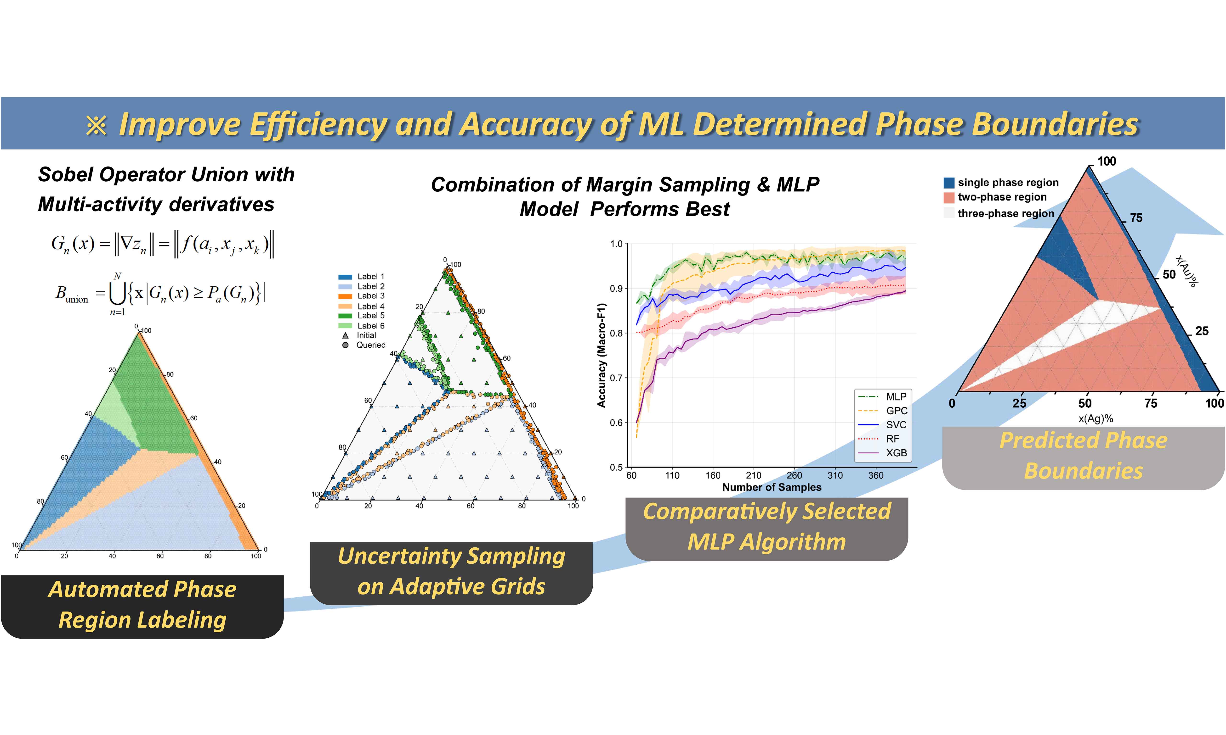
To realize the exploration of unknown diagrams directly from measurable physical/chemical properties, we improve the property derivatives-based machine learning (ML) framework of phase boundary prediction to overcome prior limitations in signal enhancement, labeling efficiency, uncertainty quantification, and potential applicability to multicomponent composition spaces. An automated phase-region labeling approach combining multiple activity derivatives is introduced to amplify the differentiability signal near phase boundaries, enabling precise identification of distinct phase regions. Three uncertainty sampling (US) strategies, i.e., least confidence (LC), margin sampling (MS), and entropy-based acquisition (EA), are employed to guide query selection in active learning. MS generally promoted a more uniform distribution of queries along phase boundaries and reduced redundant sampling near triple junctions, thereby facilitating efficient convergence. The truncated ML phase boundaries based on multi-layer perceptron + MS achieved Macro-F1 scores of 0.9994 and 0.9814 using only 120 and 186 labeled samples for the Pd-Pt and Au-Ag-Ge systems, respectively. The mean boundary displacements of ML-predicted phase boundaries against the Thermo-Calc-calculated results were 0.0059 for the Pd-Pt system and 0.0778 for the Au-Ag-Ge system.
Keywords


 Download PDF
INTRODUCTION
Phase diagrams are crucial for designing the chemical compositions and phase structures of new alloys[1]. In recent years, machine learning (ML) has been widely applied to predict phase equilibria and phase boundaries[2-4] by creating ML energy/topological functionals[5-8] and performing automatic parameter optimization[9,10], or by statistically analyzing geometric, physical, and chemical properties[11-16]. These methods have significantly sped up phase diagram analysis. However, most concentrate on reconstructing known phase boundaries or diagrams with greater accuracy. Few strategies are reported for using ML to investigate an unknown phase diagram based only on experimentally measurable physical or chemical properties.
A property-derivatives-based sampling and classification prototype was previously proposed to estimate phase boundaries directly from activity derivatives[17]. It fully leveraged the universal principle that the derivability of the system’s physical and chemical properties changes abruptly in the neighborhood of the phase boundary and developed a virtual scenario that fully simulates the experimental process of determining an unknown phase diagram using assessed activity data. This method directly couples physical and chemical properties to phase boundaries, thereby circumventing the need to model and minimize Gibbs free energy[18,19], making it particularly useful for users primarily interested in phase boundary and composition data at specific chemical points but without the experience in CALPHAD database development. Nevertheless, the prior study had four limitations: (1) it employed a single-component activity derivative to define the phase region descriptor, which failed to capture the different differential coefficients in the left and right neighborhoods, leading to insufficient signal enhancement at phase boundaries in a multi-component system; (2) it required additional manual assistance to complete the labeling process; (3) the prediction confidence score was assessed on a predefined testing grid, rather than on probability-based uncertainty measures derived from model predictions. The effects of different uncertainty acquisition criteria on sampling efficiency were therefore not systematically investigated; (4) it employed a support vector machine as the classifier, which was based on Euclidean distance and could lead to mathematical inaccuracies in high-dimensional Simplex compositional spaces.
To overcome these limitations, this study further develops a derivatives-based framework that combines automated phase region labeling from multiple activity derivatives with pool-based active learning. We compare uncertainty sampling (US) methods[20-25] for multicomponent activity derivatives within adaptive-grid active learning[25-28], aiming to build phase boundaries more effectively and reliably. The sampling and ML steps include: (1) collecting data from the pool of activity derivatives; (2) automated labeling of phase regions; (3) ML predicting phase boundaries and estimating uncertainty based on confidence; (4) re-sampling within the adaptive grid and updating models. These steps (3) and (4) are repeated until a specific convergence or accuracy goal is reached. Finally, the best ML algorithms, labeling approaches, and US strategies are summarized and justified. All these are detailed in Figure 1.
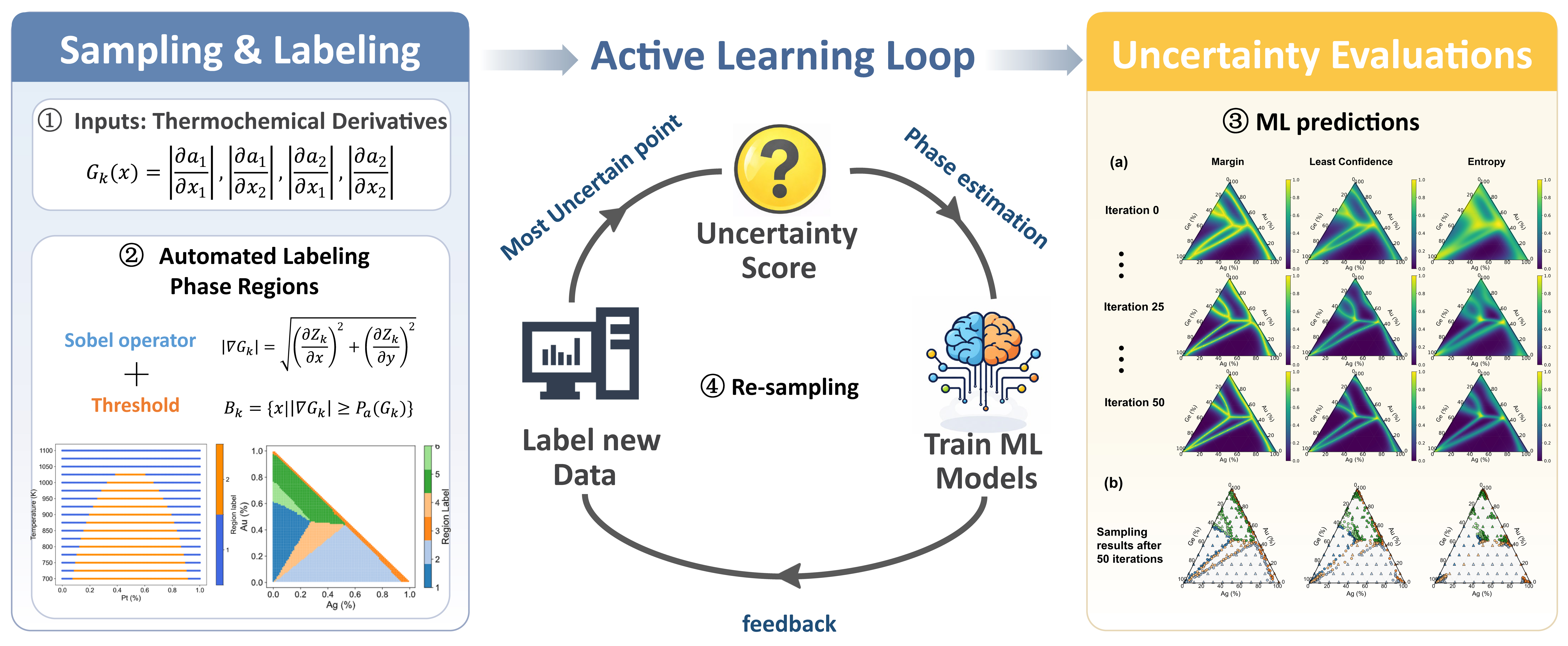
Figure 1. Technical roadmap of active learning to determine phase boundaries, and the highlights of automated labeling and uncertainty evaluation. ML: Machine learning.
MATERIALS AND METHODS
Thermodynamic fundamentals of derivative-based ML method
Based on the thermodynamics of phase diagrams, the Gibbs energy of a multi-phase system is the minimum curve that envelops the Gibbs energy of single phases and the common tangent lines/planes. It is continuous overall, but exhibits a “cusp” (i.e., a non-differentiable point) at the phase boundary composition. Therefore, by sampling the derivative of activity as a function of composition and numerically detecting the position where differentiability is lost, the phase boundary can be iteratively approximated. More details can be found in Ref.[17].
Automated phase-region labeling
In our previous work[17], phase regions were identified using a single activity derivative. This approach is effective when the selected derivative exhibits clear discontinuities at phase boundaries. In a multicomponent system, however, the sensitivity of an activity derivative depends on both the selected component and the independent composition direction. Consequently, a single derivative may detect only part of the phase boundaries and may require manual assistance to complete the phase-region labels. To address this limitation, the present method combines multiple activity-derivative channels and performs boundary extraction and region labeling algorithmically, without manual boundary drawing or point-by-point label assignment. The Pd-Pt binary system employs two derivative channels of z1 =
To quantify the spatial variation of the derivative signals, the Sobel operator[29] was applied to each derivative field. For a given activity-derivative channel zk(x), the gradient magnitude was calculated as
where u and v denote the two independent coordinates of the corresponding calculation domain. The gradient magnitude Gk(x) characterizes the local variation of the activity-derivative field and highlights regions with strong thermodynamic contrast.
To identify potential phase-boundary locations, grid points x whose exceed a percentile-based threshold Pa(·) (an adaptively chosen threshold that highlights regions with high derivative contrast) are classified as boundary pixels. The percentile level controls the balance between boundary completeness and noise suppression. A lower percentile retains weaker gradient responses and improves boundary continuity, but may introduce noise and fragmented regions. A higher percentile suppresses spurious boundaries, but may remove weak boundary segments and merge adjacent regions. For each available derivative channel k, the corresponding boundary candidate set is formulated as
To balance these effects, the search was initialized at 90% and performed bidirectionally from 80% to 98% in increments of 0.25 percentage points. The optimal percentile was selected from the interval where the fused region topology remained stable, with preference for fewer fragmented regions and proximity to 90%. Thermo-Calc phase labels were not used during threshold selection.
Therefore, the final phase boundary can be created through a geometric union of all candidate sets Bk, which combines signals from various derivatives and enhances subtle boundary features
where K = 2 for Pd-Pt system and K = 5 for Au-Ag-Ge system. Although the labeling procedure is fully automated, a final expert inspection is recommended to identify possible artifacts associated with limited grid resolution, weak derivative signals, or extremely narrow phase regions.
Data pool construction
In this study, we illustrate the US scheme using the same benchmark cases as in Ref.[17], specifically the miscibility gap boundary of fcc#1+fcc#2 on the Pd-Pt binary isopleth (700-1,100 K)[30], and the isothermal section of the Au-Ag-Ge ternary system at 800 K[31]. The original data pool comprises the independent chemical compositions, xj, the activity of component i of the system, ai (i ≤ n, j ≤ n - 1, n is the component number), and the corresponding activity derivatives
To construct a sufficiently dense and representative sampling space, the compositional domain was discretized with a uniform resolution. For the Pd-Pt system, Pt composition and temperature were used as the independent variables. The Pt composition range of 0-1 was discretized at an interval of 0.01 in mole fraction, while the temperature range of 700-1,100 K was discretized at an interval of 25 K. The complete grid therefore contained 1,717 state points. After excluding 50 uniformly distributed initial training samples, the candidate pool contained 1,667 unlabeled points. For the Au-Ag-Ge ternary system, the compositions of Au (xAu) and Ag (xAg) were used as the independent variables and discretized at intervals of 0.01. The valid compositional domain was defined under the constraint of xAu + xAg + xGe = 1, and shaped into the triangle composition simplex. xAu varied from 0.01 to 0.99, and for each xAu, xAg varied from 0 to 1 - xAu. Thus, discretization of this domain produced 5,049 valid state points. After selecting 66 uniformly distributed points for initial training, the candidate pool contained 4,983 unlabeled points. This pool serves as the ground-truth reservoir from which a small subset of labeled samples is progressively drawn during the active learning process, thereby simulating realistic experimental data acquisition under limited labelling budgets.
During each active-learning iteration, five samples were selected from the candidate pool, labeled, and transferred to the training set. Therefore, after iteration r, the numbers of training and candidate samples were
and
respectively, where N0 is the number of initial training samples (N0 = 50 for Pd-Pt system, N0 = 66 for Au-Ag-Ge system). Queried samples were removed from the candidate pool to prevent repeated selection.
ML models and US strategy
In this study, ML models are employed with the explicit objective of efficiently reconstructing equilibrium phase boundaries from limited thermodynamic information. Gaussian process classifier (GPC, kernel-based)[32] and multi-layer perceptron (MLP, neural network-based)[33] approaches were adopted to train the ML models, while random forest (RF), eXtreme gradient boosting (XGB), and support vector classifier (SVC) in the previous work served as the counterparts. These models were trained on labeled datasets and iteratively updated as new informative samples were acquired. The hyperparameters of individual ML models are displayed in Supplementary Materials 1. Brier scores and expected calibration errors (ECE) were employed to evaluate the probability calibration of the underlying models.
To emulate the active learning process in practical phase-diagram construction, several dozen data points were first uniformly sampled from the pool and assembled into the initial training dataset, representing the first round of data acquisition in practical phase-diagram exploration. The remaining data served as unlabeled candidates for query selection in each active learning cycle (analogous to the supplementary data in the second or third rounds of experiments). Table 1 details the size of the candidate pool and the initial training set for Pd-Pt and Au-Ag-Ge systems.
Size of datasets and number of decision labels for Pd-Pt and Au-Ag-Ge systems
| System | Initial training set | Candidate pool | Truncated samples | Decision labels |
| Pd-Pt | 50 | 1,667 | 120 | 2 |
| Au-Ag-Ge | 66 | 4,983 | 186 | 6 |
During each iteration, query selection was guided by uncertainty evaluations. Three uncertainty acquisition strategies, i.e., least confidence (LC), margin sampling (MS), and entropy-based acquisition (EA), were employed. For each candidate point x, an uncertainty score u(x) is computed from predicted probabilities P(y|x), and points with the highest uncertainty are selected:
where u(x) depends on the specific acquisition criterion. Then, three strategies define u(x) as follows:
and
where P(y1|x) and P(y2|x) in uMS(x) denote the highest and second-highest probabilities. The LC score measures the lack of confidence in the most probable class, MS score measures the ambiguity between the two most probable classes, and EA considers uncertainty across the complete class-probability distribution.
To avoid redundant sampling concentrated in a small local region of the compositional space, a diversity-aware batch selection strategy[34] was adopted. In each iteration, the 25 points with the highest uncertainty scores were first identified as candidate queries. The most uncertain point was selected first, after which the remaining points were selected successively by maximizing their minimum distance from the labeled set and the samples already selected in the current batch. This procedure produced a batch of five spatially diverse queries. These five points were labeled, removed from the candidate pool, added to the training set, and used to update the model.
Model evaluation and convergence criteria
Model performance was evaluated using standard classification metrics such as Accuracy, Precision, Recall, and Macro-F1 score[35]. All performance metrics were calculated over the entire data pool, rather than solely on the training subset. This evaluation protocol directly reflects the accuracy of the reconstructed phase boundaries across the full compositional domain and ensures a fair and comprehensive assessment of the active learning process. Given true positives (TP), true negatives (TN), false positives (FP), and false negatives (FN), respectively, the Macro-F1 score can be calculated as follows:
and
where C is the number of phase-region classes. Among these metrics, the Macro-F1 score was adopted as the principal classification metric because it assigns equal importance to all phase labels and is therefore less affected by differences in the sizes of individual phase regions.
However, classification-based metrics do not fully characterize the geometric fidelity of reconstructed phase boundaries. Therefore, boundary-specific validation was performed against CALPHAD-calculated equilibrium boundaries obtained using Thermo-Calc. Let Bpred and Bref denote the boundary-point sets extracted from the reconstructed and reference phase diagrams, respectively. The mean boundary displacement was calculated for both systems as the average symmetric nearest-neighbor distance:
Here, p represents a boundary point in Bpred, whereas q represents a boundary point in Bref. Lower DMBD values indicate closer agreement between the reconstructed and reference boundaries. For the Au-Ag-Ge system, triple-junction error was additionally evaluated because multiphase junctions represent the most topologically complex regions of the phase diagram. Let Jpred and Jref denote the sets of predicted and reference triple-junction locations, respectively. The triple-junction error was calculated as
where u and v represent individual junction locations in Jpred and Jref, respectively. ||·||2 denotes the Euclidean distance after geometric embedding of the phase-diagram coordinates. Thus, for the ternary system, each composition point was mapped from the composition simplex to two-dimensional equilateral-triangle coordinates before distance calculation:
where r denotes the two-dimensional Cartesian position vector of a composition point after mapping the ternary simplex onto an equilateral triangle. These reference results were used exclusively for external validation and were not involved in automated labeling, model training, internal testing, or query selection.
For convergence criteria, Macro-F1 thresholds of 0.98 for Pd-Pt and 0.95 for Au-Ag-Ge were used as initial performance targets for comparing sampling efficiency. Achieving them required fewer iterations than the final truncation criteria. Sampling proceeded until the Macro-F1 scores reached above reference level, then continued until the Macro-F1 improvement was less than or equal to 0.001 over five consecutive iterations, at which point sampling was truncated. The total number of labeled samples at termination, including both the initial training set and subsequently queried samples, was recorded as the final truncated sample number for phase-diagram reconstruction. Following this idea, the number of final samples is reported in Table 1.
The main comparisons were conducted using uniformly distributed initial training samples to ensure identical starting conditions among the models and acquisition strategies. Meanwhile, to quantify the sampling uncertainty arising from the selection of the initial labeled samples, each model-acquisition combination was additionally repeated using ten independently generated class-stratified random initial training sets of the same size.
RESULTS AND DISCUSSION
Automated phase-region labeling result
Figure 2 presents the labeled phase regions of the entire data set without using ML. Notably, the amount of data required for active learning in the real experiments is considerably smaller than that of the full data pool. The purpose of this is to demonstrate, from a bird’s-eye view, that combining multiple activity derivatives enables complete segmentation of phase regions and boundary detection without losing thermodynamic signals.

Figure 2. Partial derivatives of activities and their union result. (A-C) Pd-Pt system; (D-I) Au-Ag-Ge system.
For the Pd-Pt binary, a single-component activity derivative (
In contrast, none of the individual z1-z5 channels can independently achieve complete phase-region segmentation for the Au-Ag-Ge ternary system, as shown in Figure 2D-I. It should be emphasized that the composite channel z5 does not introduce new thermodynamic information or generate boundary features that are entirely absent from any individual channel. Instead, weak boundary responses may occur at spatially consistent locations across several derivative channels but remain fragmented or below the effective detection threshold in each individual map. By averaging the normalized derivative channels, these spatially consistent responses are retained and accumulated, whereas channel-specific fluctuations are partially suppressed. After subsequent Sobel-gradient calculation and percentile-based thresholding, some previously weak boundary segments become more continuous and distinguishable. Nevertheless, z5 alone is insufficient to recover the complete phase-boundary topology. The final segmentation is obtained by geometrically combining the candidate boundary sets from all available derivative channels, followed by region assignment based on connectivity and distance criteria. More evidence can be found in Supplementary Materials 2.
Effectiveness of active learning on phase diagram prediction
Figure 3 summarizes the performance of US strategies combined with ML models for reconstructing the miscibility-gap boundary in the Pd-Pt binary system. As shown in Figure 3A-C, the Macro-F1 scores generally increase as additional labeled samples are acquired during active learning. Across most acquisition strategies, GPC and MLP achieved higher and more stable Macro-F1 scores than the SVC, RF, and XGB models evaluated in our previous study[17]. A direct comparison in Figure 3D-F reports the number of labeled samples required by each model to reach a Macro-F1 score of 0.98. Both GPC and MLP achieve this performance using only 60 labeled samples under all three sampling strategies. Although SVC also reached the target with 60 samples under LC and EA, it required 100 samples under MS and exhibited more pronounced fluctuations during subsequent iterations.

Figure 3. Comparison of the performance of different uncertainty sampling strategies and ML models on the Pd-Pt system. (A-C) Evolution of Macro-F1 score with increasing training samples; (D-F) Number of labeled samples required by each model to reach a Macro-F1 score of 0.98. US: Uncertainty sampling; ML: machine learning; MLP: multi-layer perceptron; GPC: Gaussian process classifier; SVC: support vector classifier; RF: random forest; XGB: eXtreme gradient boosting.
The differences among LC, MS, and EA are relatively limited for the Pd-Pt system. This result can be attributed to its simple phase-region topology and the pronounced thermodynamic contrast across the miscibility-gap boundary. Because the activity-derivative signals already provide a clear distinction between the two-phase regions, the samples selected by different uncertainty criteria tend to concentrate near similar boundary locations. Consequently, the choice of acquisition strategy has a smaller influence on sampling efficiency for this binary system than the choice of ML model.
The Au-Ag-Ge ternary system represents a substantially more challenging scenario for phase-boundary reconstruction than the Pd-Pt binary case. The performance of active learning on the Au-Ag-Ge ternary system is summarized in Figure 4. Note that all model-acquisition combinations in Figures 3 and 4A-C were intentionally continued to the same maximum number of labeled samples (200 for Pd-Pt, 396 for Au-Ag-Ge) to facilitate comparison of longer-term learning behavior and this range is distinct from the final truncated sample number used for phase-diagram reconstruction.

Figure 4. Comparison of the performance of different uncertainty sampling strategies and ML models on the Au-Ag-Ge system. (A-C) Evolution of Macro-F1 score with increasing training samples; (D-F) Number of labeled samples required by each model to reach a Macro-F1 score of 0.95. US: Uncertainty sampling; ML: machine learning; MLP: multi-layer perceptron; GPC: Gaussian process classifier; SVC: support vector classifier; RF: random forest; XGB: eXtreme gradient boosting.
Compared with the Pd-Pt system, the ternary system further confirms the advantages of probability-based models. MLP and GPC again outperform RF, XGB, and SVC in both convergence speed and final accuracy. The increased complexity of the compositional simplex requires reliable probability estimates to distinguish narrow phase regions and interconnected boundaries. Probabilistic models can provide such estimates, enabling US to focus effectively on informative compositions. Furthermore, the acquisition strategies exhibit more pronounced differences, reflecting greater heterogeneity in uncertainty across the ternary compositional domain. Figure 4D-F reports the minimum number of labeled samples required to reach a Macro-F1 score of 0.95. Among these US strategies, MS generally exhibits superior performance. Under MLP, MS requires a comparable, albeit slightly larger, number of samples than LC and EA to achieve the target Macro-F1 score. In contrast, MS demonstrates a pronounced advantage for GPC, SVC, and RF, requiring substantially fewer labeled instances.
To assess the sampling uncertainty of the initial labeled samples, each model-acquisition combination was repeated ten times using class-stratified random initial sets with seeds 11, 22, 33, 44, 55, 66, 77, 88, 99, and 110. Results are shown in Supplementary Materials 3. The performance trends from these randomized samples align with those from the uniformly distributed initial samples used in the main experiments. This consistency confirms that the main conclusions are robust across different initial sampling schemes, though remaining variability is influenced by phase-diagram complexity, the underlying model, and the acquisition strategy. In addition, the benchmarks of the random sampling strategy and the results of other baseline tests are shown in Supplementary Materials 4.
Analysis of uncertainty distributions in compositional space
Since the US relies heavily on predicted class probabilities, the probability calibration of MLP, GPC, and SVC was assessed using uniformly initialized training sets before active querying. Figure 5A and B show that MLP aligns more closely with the diagonal reference line, indicating more reliable probability estimates. In contrast, GPC and SVC tend to be under-confident, especially for Au-Ag-Ge. Figure 5C and D present calibration metrics, including the multiclass Brier score and ECE. For Pd-Pt, MLP achieved a Brier score of 0.0484 and an ECE of 0.0082, while GPC and SVC scored 0.0735/0.0760 and 0.0641/0.0656, respectively. For Au-Ag-Ge, the Brier scores were 0.1299, 0.3550, and 0.2579; ECE values were 0.0162, 0.1982, and 0.1840 for MLP, GPC, and SVC. The detailed calculation procedures are provided in the Supplementary Materials 5.
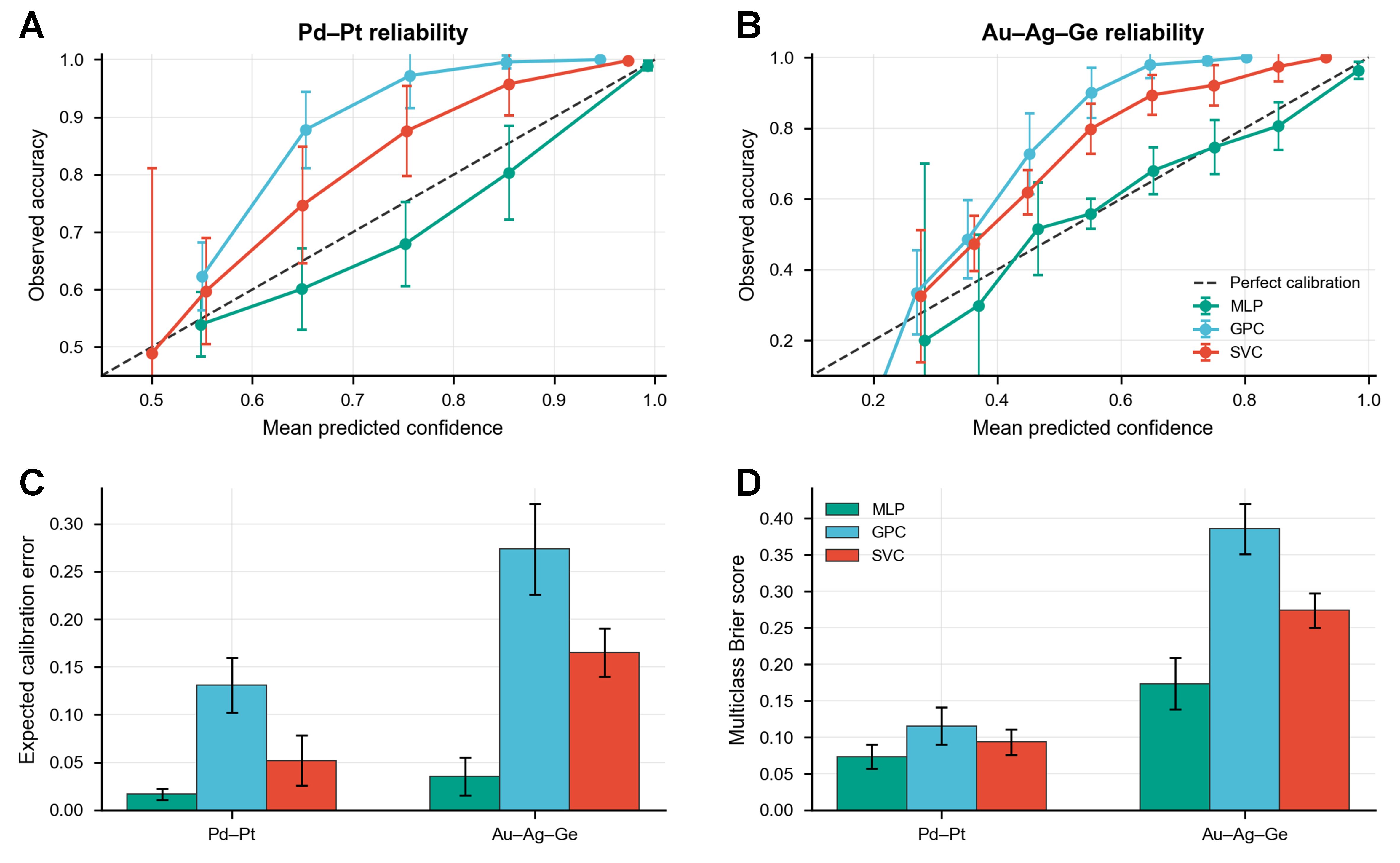
Figure 5. Probability calibration of MLP, GPC, and SVC under uniform initialization. (A and B) Reliability diagrams for Pd-Pt and Au-Ag-Ge systems, respectively; (C) Multiclass Brier scores; (D) ECEs. MLP: Multi-layer perceptron; GPC: Gaussian process classifier; SVC: support vector classifier; ECEs: expected calibration errors.
Figure 6 shows the uncertainty heat maps for the Au-Ag-Ge system after 25 iterations of active learning by examining the uncertainty landscapes generated by different combinations of ML algorithms and uncertainty acquisition strategies. Across all acquisition strategies, the heat maps reveal that regions of high predictive uncertainty consistently emerge along the phase boundaries. Regarding ML algorithm dependence, the MLP maintains relatively consistent performance across all three uncertainty strategies. It produces a smooth multi-class probability distribution using the Softmax function, with uncertainty concentrated near true phase boundaries or sparse regions, while most areas show high confidence with classification probabilities close to 0 or 1. In contrast, GPC and SVC rely on kernel-based decision functions that are sensitive to local data structure. These models tend to produce broader or fragmented uncertainty regions, particularly in areas with sparse training data.

Figure 6. Uncertainty heat maps of the Au-Ag-Ge system after 25 iterations under different ML algorithms and uncertainty acquisition strategies. Rows correspond to MLP, GPC, and SVC, while columns correspond to MS, LC, and EA. The color scale represents the normalized uncertainty score, with higher values indicating greater predictive uncertainty. ML: Machine learning; MLP: multi-layer perceptron; GPC: Gaussian process classifier; SVC: support vector classifier; MS: margin sampling; LC: least confidence; EA: entropy-based acquisition.
In US strategies, EA shows strong localized uncertainties at triple junctions due to the simultaneous and competitive labeling of three-phase regions, leading to redundant queries in the early steps of the active learning process. This slows down global phase boundary coverage and delays model convergence. This behavior arises because EA evaluates uncertainty based on global information of the predicted probability distribution. LC exhibits a more diffuse uncertainty distribution at phase boundaries. The uncertainty concentration is noticeable near the triple junctions, but lower than that of EA. The tendency stems from the fact that LC evaluates uncertainty solely based on the maximum predicted class probability Pmax, without explicitly distinguishing between binary ambiguity at phase boundaries and multi-class ambiguity at the triple junctions. Therefore, LC partially alleviates the excessive local query observed in EA sampling but remains less effective in promoting uniform coverage of phase-boundary regions. In contrast, MS produces a more uniform uncertainty distribution along phase boundaries, as it evaluates uncertainty primarily through the probability gap between the two most likely classes |p1 - p2|, making it more sensitive to the competition between labels of two-phase regions across the phase boundary and less attracted to multi-class ambiguity at triple junctions. Consequently, MS discourages oversampling at triple junctions and accelerates convergence by targeting more informative regions of the phase diagram. In this context, MS is recommended as the preferred uncertainty strategy. Overall, the MLP is recommended among the tested ML algorithms.
To further illustrate this pattern, SVC is employed as a representative example. Figure 7A displays the uncertainty heatmaps at iterations 0, 25, and 50 for MS, LC, and EA, respectively. As iterations proceed, the uncertainty distributions gradually shrink toward the true phase boundaries, reflecting the progressive refinement of the classifier. However, the evolution patterns differ markedly among the strategies. Under EA, high-uncertainty regions remain clustered near triple-junction points even at later iterations, indicating persistent localized sampling. LC shows moderate improvement but still lacks clear boundary-focused concentration. In contrast, MS progressively forms narrow and continuous high-uncertainty bands that align closely with the true interfaces, demonstrating more effective guidance for sample selection. Figure 7B further confirms these trends by visualizing the final queried sample locations. Samples selected under MS are distributed uniformly along the phase boundaries, forming coherent trajectories that cover all critical regions of the compositional simplex. EA and LC, on the other hand, exhibit more scattered and uneven sampling patterns, with noticeable oversampling in junction areas and insufficient coverage of extended boundaries.

Figure 7. Evolution of predictive uncertainty and final sampling distributions for SVC under different acquisition strategies. (A) Uncertainty distributions at iterations 0, 25, and 50 for MS, LC, and EA; (B) Sampling distributions after 50 iterations. Triangles denote the uniformly distributed initial labeled samples, whereas circles denote samples subsequently selected through active-learning queries. SVC: Support vector classifier; MS: margin sampling; LC: least confidence; EA: entropy-based acquisition.
In addition, algorithms based on Euclidean distance, such as SVC, face limitations when dealing with compositional data in the simplex space[36]. Selecting different combinations of independent components in a multi-component composition simplex space can cause significant distortions in phase boundary determination[37], although these effects are minor in ternary systems. Additive log-ratio (ALR)[38] and isometric log-ratio (ILR)[39] transformations remove the constraint that all compositions sum to 1; however, the introduced complexities reduce sampling efficiency [Table 2].
Comparison of different feature sets on the initial Macro-F1 scores and iterations required to first reach a Macro-F1 score of 0.95 under MS
| GPC | MLP | SVC | ||||
| Initial Macro-F1 | Iterations | Initial Macro-F1 | Iterations | Initial Macro-F1 | Iterations | |
| ALR | 0.537 | 26 | 0.721 | 29 | 0.449 | 168 |
| ILR | 0.507 | 20 | 0.693 | 17 | 0.499 | 112 |
| Au, Ag | 0.566 | 10 | 0.866 | 11 | 0.819 | 34 |
| Au, Ge | 0.548 | 12 | 0.868 | 10 | 0.832 | 26 |
| Ag, Ge | 0.550 | 14 | 0.858 | 8 | 0.840 | 28 |
Figure 8 shows the truncated phase boundaries using the recommended MLP + MS models. Triangles indicate the initially uniform samples, while circles mark later-acquired samples. The sampling points build up along the phase boundaries, especially near triple junctions, emphasizing the strategy’s focus on areas of high predictive uncertainty. The MLP + MS constructions of the Pd-Pt isopleth and the Au-Ag-Ge isothermal section in this work used 120 and 186 labeled samples, achieving Macro-F1 scores of 0.9994 and 0.9814, respectively, which are higher than the stable metrics of 0.980 and 0.927 in our previous work[17]. Meanwhile, the ML-predicted phase boundaries are validated against Thermo-Calc-calculated results by evaluating the mean boundary displacement. This shows mean boundary displacements of 0.0059 for the Pd-Pt binary system and 0.0778 for the Au-Ag-Ge ternary system. Notably, the recommended truncated sample numbers (120 for Pd-Pt and 186 for Au-Ag-Ge) are smaller than the maximum training-sample numbers intentionally displayed in Figure 3 (200 samples) and Figure 4 (396 samples), respectively, illustrating that the proposed framework can reconstruct an unknown phase diagram using substantially fewer samples once the convergence criterion is satisfied. The animations of the adaptive mesh grid in active learning are provided in Supplementary Materials 6.

Figure 8. Final Sampling distributions and ML-reconstructed phase diagrams obtained using MLP combined with MS for (A) Pd-Pt and (B) Au-Ag-Ge. The left panels show the labeled samples, where triangles represent the uniformly distributed initial samples and circles represent the subsequently queried samples; The right panels show the constructed phase regions, whose interfaces represent the ML-predicted phase boundaries. ML: Machine learning; MLP: multi-layer perceptron; MS: margin sampling.
Limitations and outlook
Several limitations of the present work should be acknowledged. (1) The automated labeling procedure remains sensitive to data quality and spatial resolution, with the percentile threshold and derivative-channel weights potentially requiring case-specific tuning; (2) While the differentiability-based concept is mathematically applicable to higher-dimensional composition space, the practical scalability in terms of data-pool size and computational cost has not yet been investigated; (3) Validation against real experimental data in small size is still ongoing and has not been accomplished in this study.
Our future research will focus on three main directions: (1) systematic studies of dimensionality scalability, including adaptive sampling and cost-control strategies for high-dimensional composition spaces; (2) extension of the MLP + MS framework to more complex systems, leveraging its advantages over SVC in handling high-dimensional Simplex data; and (3) comprehensive experimental validation to establish a robust tool for accelerated phase diagram determination in unknown material systems.
CONCLUSIONS
In summary, this study presents an integrated active learning framework for efficient phase-boundary prediction by combining automated labeling from multiple activity derivatives with uncertainty-guided sampling on an adaptive compositional grid. The proposed methodology provides a systematic and data-efficient approach for reconstructing complex phase diagrams with minimal labeled thermodynamic data. The main findings of this work are summarized as follows:
1. Automated labeling using multiple activity derivatives overcomes the limitation of single-derivative signals used in previous work, enabling more complete and reliable identification of phase regions in multicomponent systems.
2. Margin-based US effectively focuses queries on physically meaningful boundary regions and reduces redundant sampling at triple-junction areas, leading to higher sampling efficiency and faster convergence.
3. The MLP + MS configuration demonstrates superior performance compared with alternative models and strategies, achieving rapid convergence, high accuracy, and stable behavior for thermodynamics-informed phase-boundary prediction.
DECLARATIONS
Authors’ contributions
Writing - original draft, visualization, software, investigation: Chen, D.
Writing - original draft, writing - review and editing, validation, supervision, project administration, methodology, funding acquisition, conceptualization: Xu, G.
Visualization, software, investigation: Deng, B.
Validation, resources, project administration, funding acquisition, formal analysis, data curation: Chen, F.
Software, resources, project administration, funding acquisition: Wang, Z.
Supervision, resources, project administration: Xuan, C.
Writing - review and editing, resources, project administration, funding acquisition: Fang, J.
Writing - review and editing, validation, supervision, resources, formal analysis: Cui, Y.
Supervision, resources, project administration, funding acquisition: Zhang, A.
Availability of data and materials
Code and data to perform ML and reproduce figures can be accessed via https://github.com/Better-Ding/precious_metals_phase_AL. Some results supporting the study are presented in the Supplementary Materials.
AI and AI-assisted tools statement
Not applicable.
Financial support and sponsorship
The work was supported by the Major Scientific and Technological Project of Yunnan Precious Metals Laboratory (Grant Nos. YPML-2023050205 and YPML-202405020889) and Jiangsu Provincial Innovation Support Program-”Belt and Road” Innovation Cooperation Key Project (Grant No. BZ2023006). Xu, G. and Chen, F. acknowledge funding from the National Natural Science Foundation of China (Grants No. 52571010, 52371112) for digital design of novel alloys. Xuan, C. also acknowledges the National Natural Science Foundation of China (12211530416, 12002287) and the Research Development Fund of Xi’an Jiaotong-Liverpool University (RDF-22-01-011) for their funding support.
Conflicts of interest
Fang, J. and Zhang A. are affiliated with Yunnan Precious Metals Laboratory Co., Ltd., and Wang, Z. is affiliated with MatAi Co. Ltd., while the other authors have declared that they have no conflicts of interest.
Ethical approval and consent to participate
Not applicable.
Consent for publication
Not applicable.
Copyright
© The Author(s) 2026.
Supplementary Materials
REFERENCES
1. Liu, Z. Thermodynamics and its prediction and CALPHAD modeling: review, state of the art, and perspectives. Calphad 2023, 82, 102580.
2. Arróyave, R. Phase stability through machine learning. J. Phase. Equilib. Diffus. 2022, 43, 606-28.
3. Chew, P. Y.; Reinhardt, A. Phase diagrams-Why they matter and how to predict them. J. Chem. Phys. 2023, 158, 030902.
4. Shen, C. The synergy of machine learning and CALPHAD: revitalizing traditional approaches. Comput. Mater. Sci. 2025, 258, 113970.
5. Kruglov, I. A.; Yanilkin, A.; Oganov, A. R.; Korotaev, P. Phase diagram of uranium from ab initio calculations and machine learning. Phys. Rev. B. 2019, 100, 174104.
6. Rosenbrock, C. W.; Gubaev, K.; Shapeev, A. V.; et al. Machine-learned interatomic potentials for alloys and alloy phase diagrams. npj. Comput. Mater. 2021, 7, 477.
7. Zhu, S.; Sarıtürk, D.; Arróyave, R. Accelerating CALPHAD-based phase diagram predictions in complex alloys using universal machine learning potentials: opportunities and challenges. Acta. Mater. 2025, 286, 120747.
8. Xie, J. Z.; Zhou, X. Y.; Jin, B.; Jiang, H. Machine learning force field-aided cluster expansion approach to phase diagram of alloyed materials. J. Chem. Theory. Comput. 2024, 20, 6207-17.
9. Bocklund, B.; Otis, R.; Egorov, A.; Obaied, A.; Roslyakova, I.; Liu, Z. ESPEI for efficient thermodynamic database development, modification, and uncertainty quantification: application to Cu–Mg. MRS. Commun. 2019, 9, 618-27.
10. Zhang, H.; Wu, B.; Zhang, L.; Wang, H. Efficient thermodynamic modelling with uncertainty quantification of the Ag–Cu–Co system from its sub-binary systems. Mater. Chem. Phys. 2023, 308, 128276.
11. Deffrennes, G.; Hallstedt, B.; Abe, T.; et al. Data-driven study of the enthalpy of mixing in the liquid phase. Calphad 2024, 87, 102745.
12. Wu, B.; Zhang, H.; Zhang, L.; Wang, H. Estimating the temperature dependent zero-phase-fraction features in ternary phase diagram via Bayesian approach. Scripta. Mater. 2023, 235, 115615.
13. Lund, J.; Wang, H.; Braatz, R. D.; García, R. E. Machine learning of phase diagrams. Mater. Adv. 2022, 3, 8485-97.
14. Deffrennes, G.; Terayama, K.; Abe, T.; Tamura, R. A machine learning–based classification approach for phase diagram prediction. Mater. Design. 2022, 215, 110497.
15. He, J.; Su, X.; Wang, C.; et al. Machine learning assisted predictions of multi-component phase diagrams and fine boundary information. Acta. Mater. 2022, 240, 118341.
16. Terayama, K.; Han, K.; Katsube, R.; et al. Acceleration of phase diagram construction by machine learning incorporating Gibbs’ phase rule. Scripta. Mater. 2022, 208, 114335.
17. Li, H.; Xu, G.; Chen, F.; et al. Estimating phase boundaries using sampling and machine learning of derivatives of thermochemistry properties. Calphad 2026, 92, 102920.
18. Hao, L.; Ruban, A.; Xiong, W. CALPHAD modeling based on Gibbs energy functions from zero kevin and improved magnetic model: a case study on the Cr–Ni system. Calphad 2021, 73, 102268.
19. Liu, Z. K.; Wang, Y. Computational thermodynamics of materials. Cambridge University Press: Cambridge, 2016.
20. Koizumi, A.; Deffrennes, G.; Terayama, K.; Tamura, R. Performance of uncertainty-based active learning for efficient approximation of black-box functions in materials science. Sci. Rep. 2024, 14, 27019.
21. Terayama, K.; Tamura, R.; Nose, Y.; et al. Efficient construction method for phase diagrams using uncertainty sampling. Phys. Rev. Mater. 2019, 3, 033802.
22. Wu, B.; Zhang, H.; Zhou, Y.; Zhang, L.; Wang, H. Uncertainty quantification of phase boundary in a composition-phase map via Bayesian strategies. Phys. Rev. Mater. 2023, 7, 025201.
23. Liu, P.; Yu, H.; Qin, H.; et al. Construction of material phase diagram using different uncertainty estimation strategies. Mater. Lett. 2025, 384, 138036.
24. Varivoda, D.; Dong, R.; Omee, S. S.; Hu, J. Materials property prediction with uncertainty quantification: a benchmark study. Appl. Phys. Rev. 2023, 10, 021409.
25. Tian, Y.; Yuan, R.; Xue, D.; et al. Role of uncertainty estimation in accelerating materials development via active learning. J. Appl. Phys. 2020, 128, 014103.
26. Tian, Y.; Yuan, R.; Xue, D.; et al. Determining multi-component phase diagrams with desired characteristics using active learning. Adv. Sci. 2020, 8, 2003165.
27. Dai, C.; Glotzer, S. C. Efficient phase diagram sampling by active learning. J. Phys. Chem. B. 2020, 124, 1275-84.
28. Lookman, T.; Balachandran, P. V.; Xue, D.; Yuan, R. Active learning in materials science with emphasis on adaptive sampling using uncertainties for targeted design. npj. Comput. Mater. 2019, 5, 153.
29. Kanopoulos, N.; Vasanthavada, N.; Baker, R. Design of an image edge detection filter using the Sobel operator. IEEE. J. Solid. State. Circuits. , 23, 358-67.
30. Turchi, P. E. A.; Drchal, V.; Kudrnovský, J. Stability and ordering properties of fcc alloys based on Rh, Ir, Pd, and Pt. Phys. Rev. B. 2006, 74, 064202.
31. Wang, J.; Liu, Y.; Tang, C.; Liu, L.; Zhou, H.; Jin, Z. Thermodynamic description of the Au–Ag–Ge ternary system. Thermochim. Acta. 2011, 512, 240-6.
32. Deringer, V. L.; Bartók, A. P.; Bernstein, N.; Wilkins, D. M.; Ceriotti, M.; Csányi, G. Gaussian process regression for materials and molecules. Chem. Rev. 2021, 121, 10073-141.
33. Rumelhart, D. E.; Hinton, G. E.; Williams, R. J. Learning representations by back-propagating errors. Nature 1986, 323, 533-6.
34. Wang, X.; Wang, J.; Yan, C. A multi-candidate batch mode active learning approach. In Proceedings of the 2023 15th International Conference on Machine Learning and Computing. Association for Computing Machinery; 2023. pp 528-33.
35. Yacouby, R.; Axman, D. Probabilistic extension of Precision, Recall, and F1 score for more thorough evaluation of classification models. In Proceedings of the First Workshop on Evaluation and Comparison of NLP Systems. Association for Computational Linguistics; 2020. pp 79-91.
36. Heese, R.; Schmid, J.; Walczak, M.; Bortz, M. Calibrated simplex-mapping classification. PLoS. One. 2023, 18, e0279876.
37. Krajewski, A. M.; Beese, A. M.; Reinhart, W. F.; Liu, Z. Efficient generation of grids and traversal graphs in compositional spaces towards exploration and path planning. npj. Unconv. Comput. 2024, 1, 12.
38. Greenacre, M.; Grunsky, E.; Bacon-Shone, J.; Erb, I.; Quinn, T. Aitchison’s compositional data analysis 40 years on: a reappraisal. Statist. Sci. 2023, 38, 386-410.
Cite This Article
 Open Access
How to Cite
Chen, D.; Xu, G.; Deng, B.; Chen, F.; Fang, J.; Wang, Z.; Xuan, C.; Cui, Y.; Zhang, A. Multi-activity derivative automated labeling and margin-sampling active learning for efficient determination of phase boundaries. J. Mater. Inf. 2026, 6, 46. https://dx.doi.org/10.20517/jmi.2026.21
Download Citation
If you have the appropriate software installed, you can download article citation data to the citation manager of your choice. Simply select your manager software from the list below and click on download.
Export Citation File
Type of Import
Tips on Downloading Citation
Citation Manager File Format
Type of Import
Direct Import: When the Direct Import option is selected (the default state), a dialogue box will give you the option to Save or Open the downloaded citation data. Choosing Open will either launch your citation manager or give you a choice of applications with which to use the metadata. The Save option saves the file locally for later use.
Indirect Import: When the Indirect Import option is selected, the metadata is displayed and may be copied and pasted as needed.
About This Article
Copyright

Data & Comments
Data
0











Comments
Comments must be written in English. Spam, offensive content, impersonation, and private information will not be permitted. If any comment is reported and identified as inappropriate content by OAE staff, the comment will be removed without notice. If you have any queries or need any help, please contact us at [email protected].