


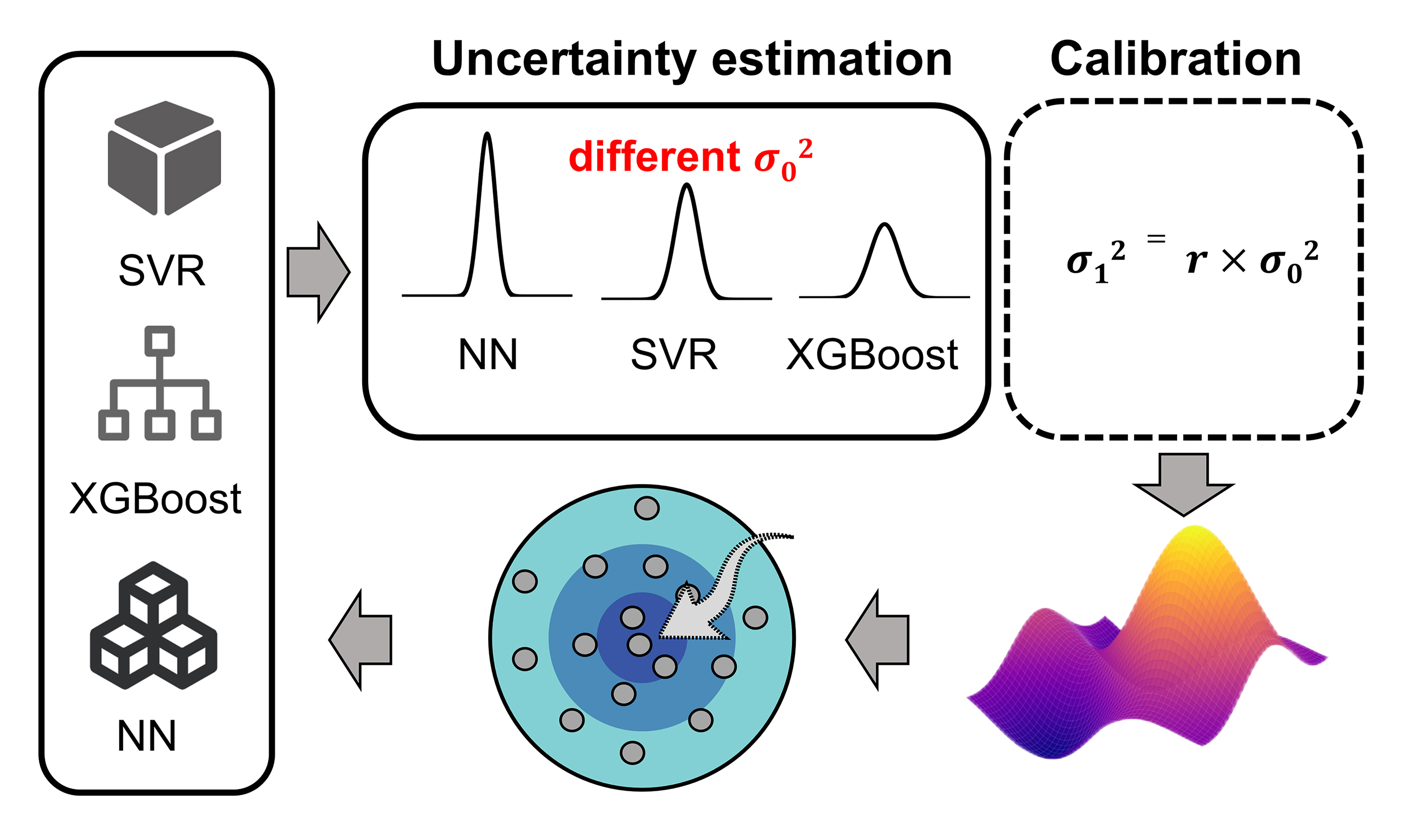
Uncertainty estimation affects predictor selection and its calibration improves materials optimization
 0
0 Abstract
Uncertainty is crucial when the available data for building a predictor are insufficient, which is ubiquitous in machine-learning-driven materials studies. However, the impact of uncertainty estimation on predictor selection and materials optimization remains incompletely understood. Here, we demonstrate that in active learning, uncertainty estimation significantly influences predictor selection, as well as that the calibration of uncertainty estimation can improve the optimization. The idea is validated on three alloy datasets (Ni-based, Fe-based, and Ti-based) using three commonly used algorithms - support vector regression (SVR), neural networks (NN), and extreme gradient boosting (XGBoost) - which yield comparable predictive accuracy. It is shown that XGBoost presents more reliable uncertainty estimation than SVR and NN. Using the directly estimated uncertainty for the three predictors with similar accuracy, we find that the optimization is quite different. This suggests that uncertainty estimation plays a role in predictor selection. The uncertainty estimation is then calibrated to improve reliability, and its effect on optimization is compared with the uncalibrated case. Among the nine cases considered (three models and three datasets), eight show improved optimization when calibrated uncertainty estimation is used. This work suggests that uncertainty estimation and its calibration deserve greater attention in active learning-driven materials discovery.
Keywords
INTRODUCTION
Active learning has been widely employed in materials science to accelerate the discovery of new materials[1-10]. It consists of a predictor to make predictions on unknown materials and a selector to select promising candidates for validation[11-16]. Generally, the choice of predictor is determined by comparing the accuracies of several surrogate models. This approach is reasonable when sufficient data are available to construct a predictor capable of capturing the underlying structure of the unexplored space[17-23]. However, the available data are often limited compared to the unknown domain, raising concerns about whether the learned surrogate model remains merely interpolative[23-26]. This limitation motivates the incorporation of uncertainty estimation into the selector, as it can facilitate exploration beyond the distribution of existing data and improve search efficiency. Consequently, uncertainty estimation and its application in active learning have attracted significant attention[7,27].
Different strategies, such as Bayesian approaches and ensemble methods, have been used to estimate the uncertainty associated with the predictor[1-3,27-32]. However, the Bayesian methods are mainly limited to Gaussian models. The ensemble methods are often based on resampling strategy and have thus been widely used across various predictors, just as the bootstrap we used in this study[2,33-36]. It has been suggested that for neural network (NN) potentials, the uncertainty estimation using a single model (even with reduced cost) does not always outperform that from model ensembles[33]. In previous work, we used a support vector machine as a base learner and compared the effect of uncertainty estimation via two methods, i.e., bootstrap and jackknife, on active learning[37]. However, two key issues remain. First, the predictor trained on limited materials data may not be reliable when applied to an unknown space. Why not use uncertainty to assist in predictor selection, rather than relying solely on accuracy over existing data? This issue becomes particularly relevant when predictors show similar accuracy but different uncertainty, such as the commonly used shallow-layer methods including support vector regression (SVR), NN and extreme gradient boosting (XGBoost)[38-42]. Second, current studies often directly use uncertainty estimation from methods such as bootstrap, lacking is to investigate how the calibration of such uncertainty estimation affects active learning, will this make the optimization more efficient? These concepts are illustrated in Figure 1.
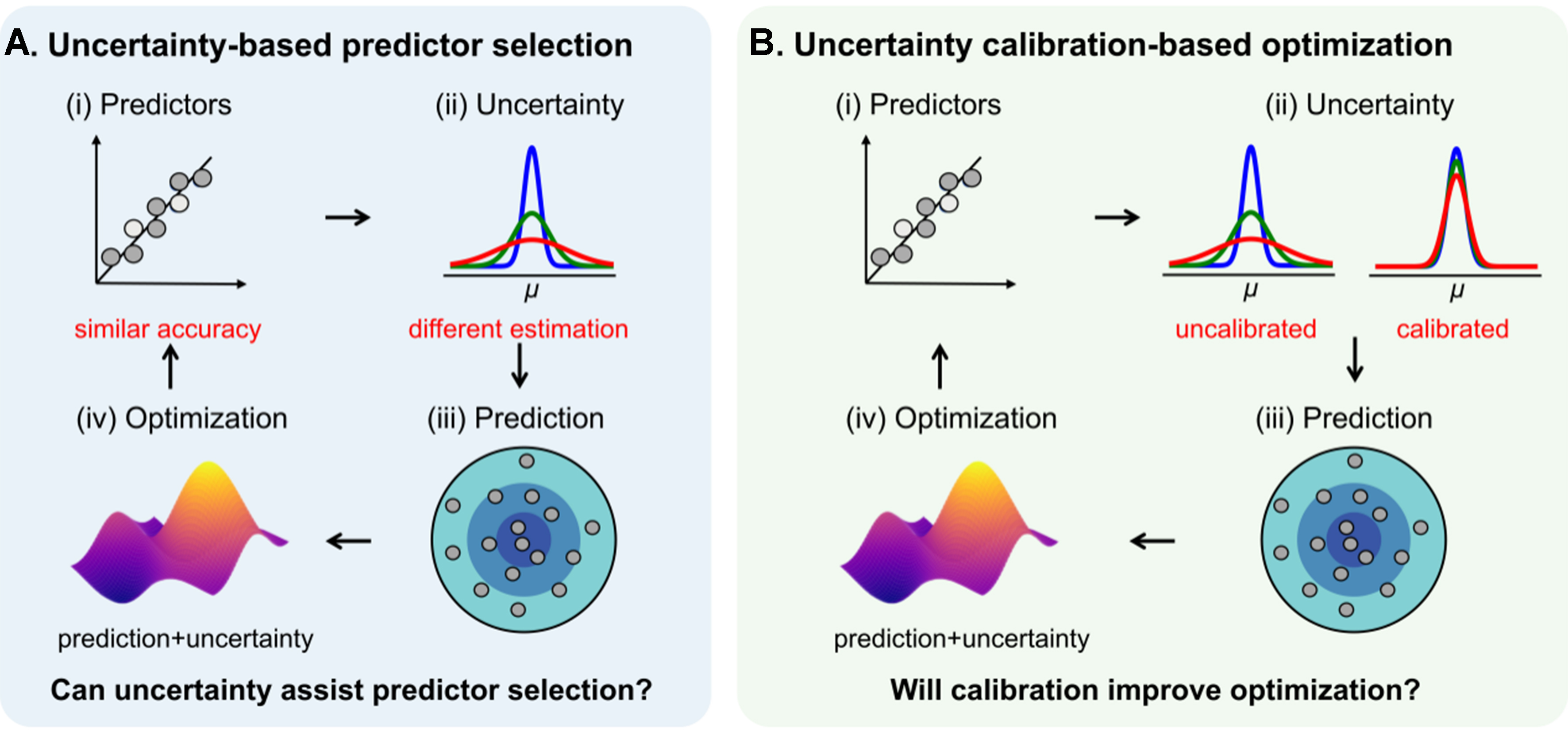
Figure 1. Schematic illustration of the concepts explored in this work: (A) uncertainty-based predictor section and (B) uncertainty calibration-based optimization.
We answer the above two questions by examining the effect of uncertainty estimation on predictor selection and its calibration on materials optimization. We demonstrate the idea on three alloy datasets. For various datasets, the predictors show similar accuracy but quite different uncertainty estimation. As a result, the materials optimization efficiency varies largely and thereby suggests that uncertainty estimation needs to be considered when determining the predictor. The effect of uncertainty estimation before and after calibration on materials optimization is also compared. It is demonstrated that 8 of 9 cases show improved optimization using calibrated uncertainty.
MATERIALS AND METHODS
Regression models
For the SVR model, the hyperparameter search range includes the regularization parameter C (0.5, 1, 1.5, 2, 3, 5, 10, 100) and kernel types [linear, polynomial, and radial basis function (RBF)]. For the XGBoost model, the tuned hyperparameters include the number of trees (100, 200, 300, 500), maximum depth (3, 5, 7), learning rate (0.01, 0.05, 0.1), subsampling rate (0.7, 0.8, 0.9), and feature subsampling rate (0.7, 0.8, 0.9). Grid search is used to determine the optimal hyperparameters for both models.
The NN consists of 100 input neurons, two hidden layers (each with 200 neurons), and uses the ReLU activation function defined by the formula Relu(x) = max(0, x), where x denotes the weighted input of a neuron. A Dropout layer with a rate of 0.5 is added after each hidden layer to prevent overfitting. The Adam optimizer is used with a learning rate of 0.02, and the model is trained for 2,000 epochs.
Active learning
The efficient global optimization is used to guide the selection of promising candidates for experimental validation, whose efficacy has been identified in a series of studies for materials discovery[43-45]. This optimal algorithm can balance the trade-off between the mean of predictions (μ(x)) and associated uncertainty (σ(x)) for a given unknown composition, which cannot only exploit new materials with desired property but also improve the surrogate model simultaneously. The selection of the most promising candidate is guided by the maximization of the expected improvement (E[I(x)]), which is defined as[46]
where μ* is the best property in the training data, z = μ(x) - μ*Yσ(x), and ϕ(z) and Ф(z) are the standard normal density function and cumulative distribution function, respectively.
Dataset
There are three alloy datasets: Ni-based, Fe-based and Ti-based, which contain 542, 173 and 88 entries, respectively. In all three datasets, the target property is creep rupture lifetime. The Ni-based and Fe-based datasets are derived from the public National Institute for Materials Science (NIMS) database (https://cds.nims.go.jp), while the Ti-based dataset is from Ref.[47]. The Fe-based and Ni-based alloy datasets contain 33 features, including 22 alloy compositions (such as C, Ni, Cr, etc.), nine solution and aging treatment parameters (time, temperature, cooling method), and two testing conditions (temperature, stress); the Ti-based alloy dataset contains 25 features, with 14 compositions (such as C, Ti, Sn, etc.), and the heat treatment parameters and testing conditions are set consistently with the first two. The datasets used are provided in the Supplementary Materials.
RESULTS AND DISCUSSION
Predictors and uncertainty estimation
We use three algorithms - SVR, NN, and XGBoost - to build the surrogate models and compare their performance. To assess the ability of the predictors, each dataset is split into a training set and a test set with a ratio 8:2. Figure 2A-C shows that for the Ni-based dataset, the average R2 (goodness of fit between predicted and actual values, closer to 1 indicates better performance) of SVR, XGBoost, and NN are 0.87, 0.85, and 0.88, respectively. On the Fe-based dataset, the average R2 of NN (0.81) is lower than that of SVR (0.91) and XGBoost (0.93), as shown in Figure 2D-F. Figure 2G-I shows that for the Ti-based dataset, the average R2 of SVR, XGBoost, and NN are 0.93, 0.91, and 0.91, respectively. We also calculate the mean absolute error (MAE) and root-mean-square error (RMSE) of the different models on the various datasets, as provided in Supplementary Table 1. Overall, almost all models show similar accuracies on the same test data across different materials. In this context, choosing a predictor based solely on accuracy is difficult, highlighting the high demand for incorporating predictor-associated uncertainty.
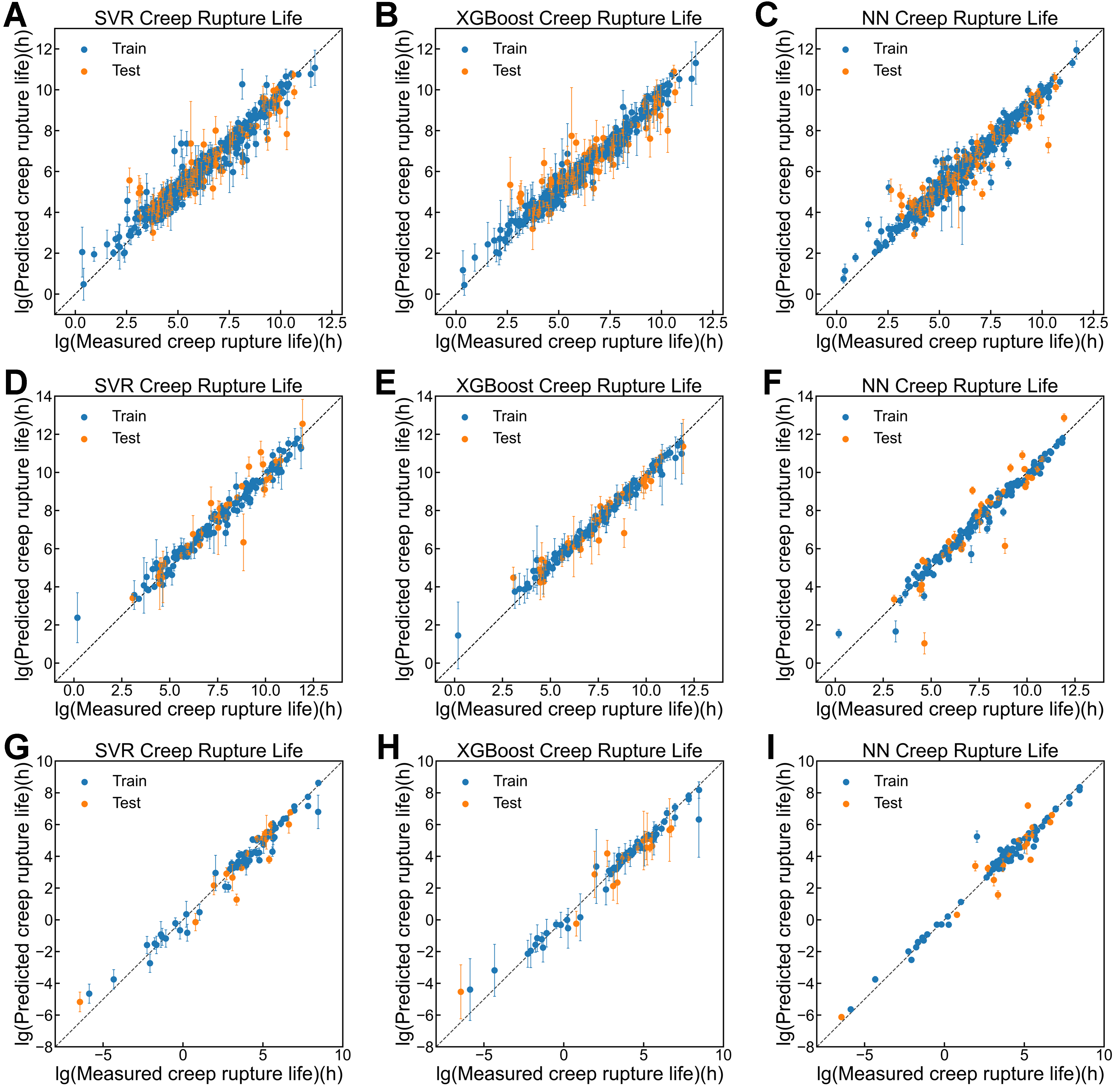
Figure 2. The performance of different models on the three datasets. (A-C) Ni-based dataset; (D-F) Fe-based dataset; and (G-I) Ti-based dataset. SVR: Support vector regression; XGBoost: extreme gradient boosting; NN: neural network.
Here, the uncertainty estimation is obtained using the bootstrap resampling method. For each diagram in Figure 2, a total of 50 surrogate models are established based on 50 datasets, each being a subset of the training data. These 50 surrogate models are applied to the test set, with each sample receiving 50 predicted values. For each sample, the mean of these predictions is calculated, and the standard deviation is defined as the uncertainty. It should be noted that the R2 values reported above are calculated using the mean predictions, taking model reliability into account.
Evaluation and calibration of uncertainty estimation
We calculate the miscalibration area and use it as an index to assess the uncertainty estimation[48,49]. The calculation of the miscalibration area is as follows. Specifically, for each test sample i, we get the predicted mean μi and the associated standard deviation σi (uncertainty) based on the predictions using bootstrap resampling. We assume that all the predictions for sample i conform to the א[μi, σi2]. We set a series of confidence levels {αk} evenly spaced between 0% and 100%. For each sample i, we compute the two confidence boundaries: Li,k = μi -
Figure 3A, D and G shows the miscalibration curves for the three different models on the Ni-based dataset (the Ti-based and Fe-based datasets are provided in Supplementary Figures 1 and 2). All three calibration curves lie below the diagonal, implying an underestimation of uncertainty. The NN exhibits particularly poor uncertainty estimation. Across different datasets, XGBoost generally demonstrates better uncertainty estimation than SVR and NN, with the ranking XGBoost > SVR > NN. As the dataset size increases - from Ti-based (88) and Fe-based (173) to Ni-based (542) - the uncertainty estimation of XGBoost shifts from overestimation to underestimation, whereas the uncertainty of SVR and NN is consistently underestimated.
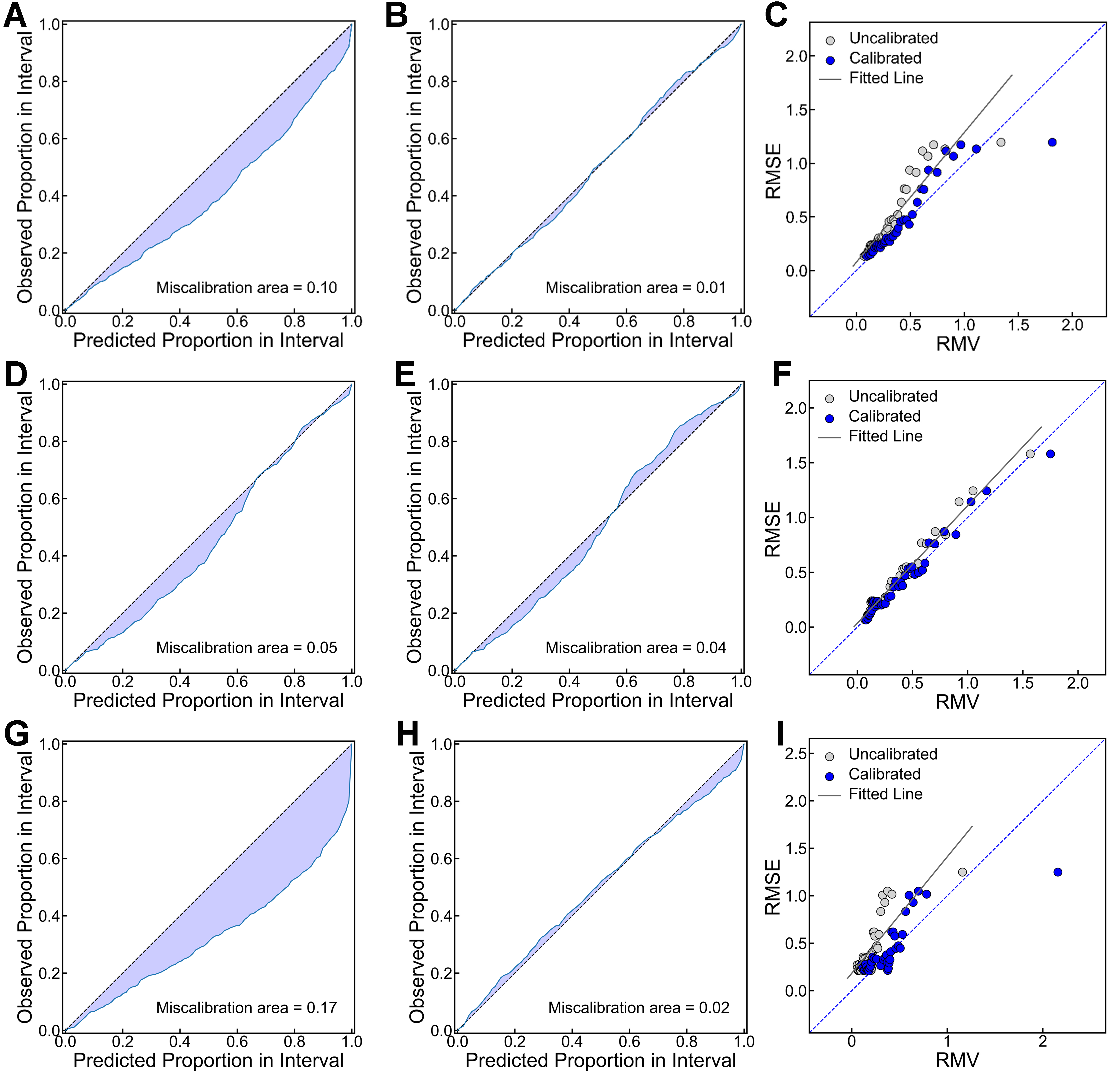
Figure 3. Uncertainty estimation and calibration on the Ni-based dataset with different models. (A), (D), and (G) Miscalibration curves for SVR, XGBoost, and NN, respectively; (B), (E), and (H) Miscalibration curves after calibration; (C), (F), and (I) Relationship between RMSE and RMV before and after uncertainty calibration. SVR: Support vector regression; XGBoost: extreme gradient boosting; NN: neural network; RMSE: root-mean-square error; RMV: root mean variance.
We next use the temperature coefficient scaling method to calibrate the uncertainty estimation to improve the reliability[50]. This method applies a scaling factor, r, to the uncertainty (i.e., r * σ). The factor r is determined by minimizing the objective function f(r) - where f(r) represents the miscalibration area for a given r - via the Brent iteration method. The search interval is initialized as [rlower, rupper], with the initial optimal estimate r0 = 1. In each iteration, a quadratic polynomial is fitted based on the current interval endpoints, rlower and rupper, and the current optimal value r0, along with their corresponding miscalibration areas, to calculate the candidate value rcandidate (the minimum point). If rcandidate is within the interval and reduces the miscalibration area, the interval is contracted according to its position (e.g., if rcandidate < r0, the new interval is [rlower, r0]), and r0 is updated to rcandidate. The next iteration refits the three points using the updated interval endpoints, the new r0, and their ordinates. If rcandidate is invalid (out of bounds or that the ordinate does not decrease), the current r0 is retained. Instead, the golden section method is used to generate two interior points r1 = rupper - 0.618(rupper - rlower) and r2 = rlower + 0.618(rupper - rlower) within the previous interval. By comparing their miscalibration area [i.e., f(r1) and f(r2)], if f(r1) < f(r2), the interval [rlower, r2] is retained. At this time, r0 remains unchanged. However, after updating the interval, the next iteration continues to repeat the above process based on the current r0, the new interval endpoints, and their ordinates until the interval width converges to |rupper - rlower| < 1.48 × 10⁻⁸. Finally, r0 is output as the global optimal solution. With the determined r, the calibrated results for the three models are shown in Figure 3B, E, and H. It can be seen that the miscalibration areas for SVR, XGBoost, and NN decrease from 0.1, 0.05, and 0.17 to 0.01, 0.04, and 0.02, respectively. Table 1 summarizes the miscalibration areas before and after calibration for the three models across different datasets. The NN model shows the largest improvement.
Miscalibration areas (MA) for the three models across different datasets before and after calibration [the model accuracy (R2) is also included]
| Dataset | Calibration | SVR | XGBoost | NN | |||
| R2 | MA | R2 | MA | R2 | MA | ||
| Ni-based | No | 0.87 | 0.10 | 0.85 | 0.05 | 0.88 | 0.17 |
| Yes | 0.01 | 0.04 | 0.02 | ||||
| Fe-based | No | 0.91 | 0.13 | 0.93 | 0.11 | 0.81 | 0.17 |
| Yes | 0.03 | 0.07 | 0.02 | ||||
| Ti-based | No | 0.93 | 0.14 | 0.91 | 0.08 | 0.91 | 0.36 |
| Yes | 0.02 | 0.05 | 0.04 | ||||
We next examine the calibration efficacy of uncertainty estimation by using another statistical method. Specifically, the correlation between RMSE and standard deviation [uncertainty, here named root mean variance (RMV) according to previous studies] is investigated[34]. For a given dataset and surrogate model, we have the RMSE and RMV of each data point. Next, all data points were ranked in ascending order using RMV. Given the large number of points, they were grouped into bins, with the number of bins determined based on the dataset size. In this context, the bins for Ti-based, Fe-based and Ni-based are 10, 20 and 40, respectively. The RMSE and RMV for the points in each bin are averaged to obtain the corresponding mean value. Figure 3C, F, and I shows the distribution of the mean values for RMSE and RMV, using the Ni-based dataset as an example. Note that distributions from both calibrated (blue) and uncalibrated (grey) uncertainties are included for comparison. Ideally, the closer the points align to the diagonal, the better the uncertainty estimation. For all three models, the blue points lie closer to the diagonal, further indicating that calibration improves the uncertainty estimation. The fitted slopes and intercepts before and after calibration are summarized in Supplementary Table 2. Results for the Ti-based and Fe-based datasets are shown in Supplementary Figures 1 and 2.
Influence of uncertainty estimation and calibration on active learning-based optimization
In the previous sections, we obtained the uncertainty estimation and then evaluated and calibrated it. As a showcase, we used only 50 bootstrap-based resampling iterations to obtain the uncertainty. In fact, the number of resampling iterations affects the uncertainty estimation. Therefore, before executing active learning, we examined the influence of resampling iterations on the uncertainty estimation. A reasonable value is expected to balance reliability and efficiency. Specifically, we investigated the change of the scaling factor r with different numbers of resampling iterations. The rationale is as follows: if the uncertainty estimation does not vary, then r will also remain unchanged. Figure 4A-C shows the r as a function of resampling iterations for the three models on the Ni-based dataset. The scaling factor r first decreases and then stabilizes as the number of resampling iterations increases. Using the SVR model as an example, r converges when the resampling reaches 200 iterations. This trend is also observed for the other two models. The error bars are obtained by repeating the resampling five times for a given number of iterations. The small error indicates that, in each round, the effect of resampling on uncertainty estimation is minimal and can be neglected. Therefore, in the subsequent active learning study, we use 200 resampling iterations to obtain the uncertainty for all three models. A similar trend is observed for the Ti-based and Fe-based datasets [Supplementary Figures 3 and 4].
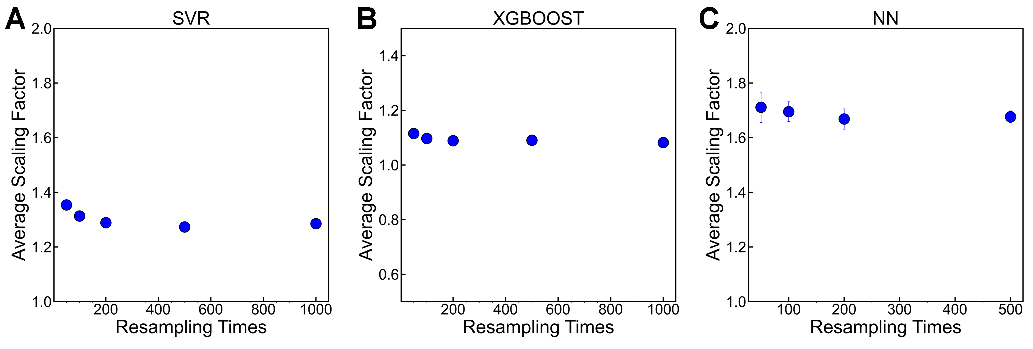
Figure 4. The change of scaling factor r with resampling iterations, using the Ni-based dataset as an example. (A) The SVR model; (B) The XGBoost model; (C) The NN model. SVR: Support vector regression; XGBoost: extreme gradient boosting; NN: neural network.
Uncertainty-based predictor selection
Assisted by active learning, we first investigate how uncertainty estimation affects predictor selection when the accuracy is similar, as shown in Figure 2 and Table 1. Similar to the data division in Section “Predictors and uncertainty estimation”, the data are split into training and test sets in an 8:2 ratio. In this subsection, the test set is not used; however, in the next subsection, it will be used to calibrate the uncertainty estimation. To fairly compare the optimization efficiency before and after uncertainty calibration, the test set is excluded from the active learning loop.
The active learning loop starts with 10% of the training data, while the remaining 90% serves as the unexplored space where the property is assumed unknown. The initial 10% is not randomly selected; instead, the training data are ranked based on the creep rupture lifetime, and the 10% with the lowest property values are chosen as the starting set. Using this data, three surrogate models are built to make predictions on the unexplored samples. Next, the expected improvement (EI) criterion is employed to recommend a candidate with the highest potential to improve the target property. This candidate is then added to the initial 10%, the models are retrained, and the loop iterates for the next round. The iteration stops when the sample with the best property is identified. Opportunity cost (OC) is used to evaluate how closely the recommended sample approximates the best sample during the iterations. OC is defined as the absolute difference between the maximum in the training set and the maximum in the combined dataset (training set plus unexplored space).
The green curves in Figure 5 show the evolution of OC with iteration for the three models across the three alloy datasets. It is evident that, for a given dataset, even when predictors exhibit similar accuracy, the optimization efficiency can vary significantly, supporting our first assumption in the introduction. For the Fe-based dataset in Figure 5D-F, the miscalibration areas of the three models are ranked as NN > SVR > XGBoost, indicating that XGBoost has the most reliable uncertainty estimation, followed by SVR and NN. Accordingly, the optimization efficiency is XGBoost > SVR > NN, consistent with our results. For the other two datasets, the optimization efficiency exhibits the opposite trend relative to the uncertainty estimation. Nevertheless, these findings clearly suggest that when predictors show similar accuracy, uncertainty can serve as a useful index for selecting the most appropriate model. We envision that this comparison not only aids predictor selection under similar accuracy conditions but also challenges the traditional practice of relying solely on accuracy.
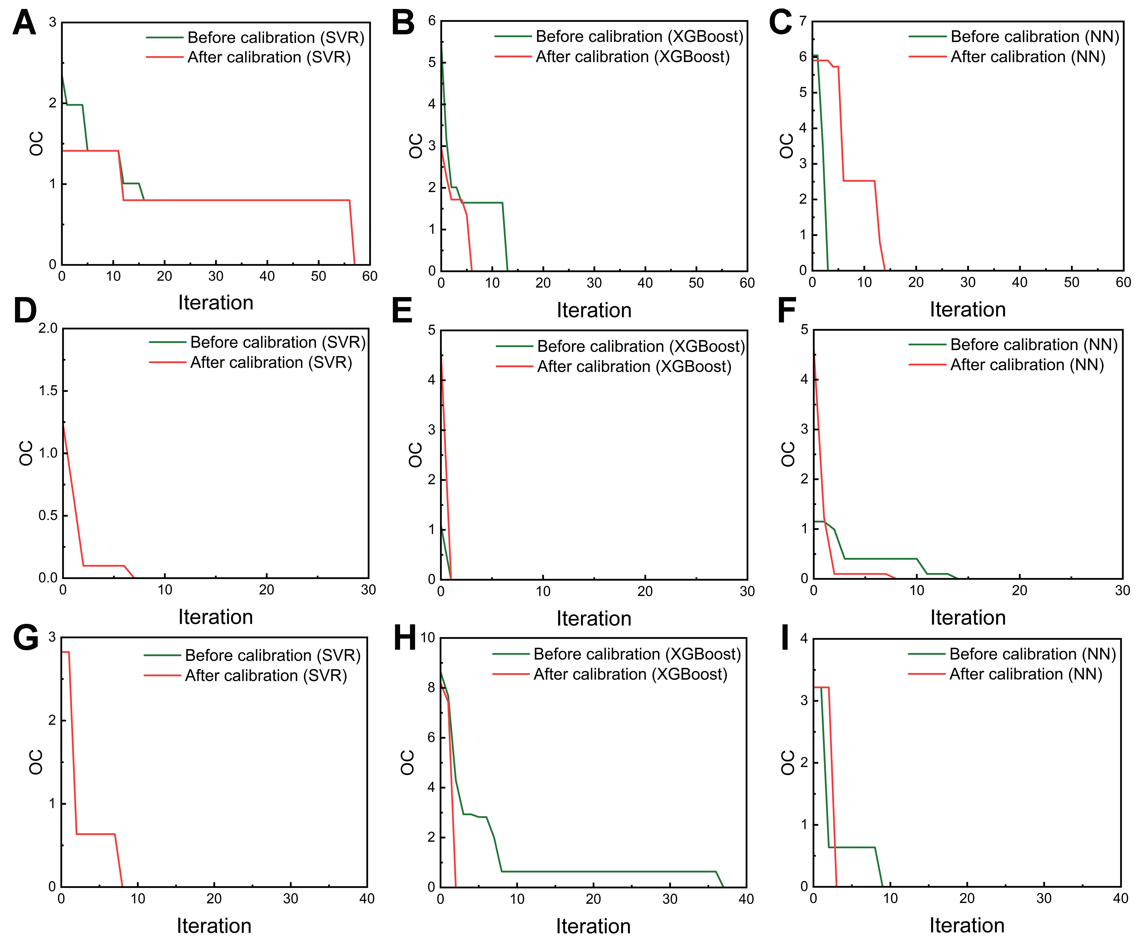
Figure 5. Changes in OC during iteration across different datasets: (A-C) Ni-based dataset with (A) SVR, (B) XGBoost, and (C) NN; (D-F) Fe-based dataset with (D) SVR, (E) XGBoost, and (F) NN; (G-I) Ti-based dataset with (G) SVR, (H) XGBoost, and (I) NN. In panels (D) and (G), the two curves overlap completely, indicating identical OC evolution behaviors. OC: Opportunity cost; SVR: support vector regression; XGBoost: extreme gradient boosting; NN: neural network.
Uncertainty calibration-driven optimization
We next investigate how the calibration of uncertainty estimation affects active learning-based optimization. The red curves in Figure 5 show the evolution of optimization with calibrated uncertainty. Note that for the calibrated case, the uncertainty is calibrated for each iteration using the evolving training data and test data. For the Fe-based and Ti-based datasets in Figure 5, it is seen that for all three models, the optimization efficiency is improved, indicating that calibration of uncertainty estimation can accelerate the search of unexplored space. For the Ni-based dataset, Figure 5A shows that the optimization efficiency of SVR improves in the initial iterations, although the final convergence point remains nearly unchanged, while Figure 5B demonstrates a clear improvement in the optimization efficiency of XGBoost. In summary, 8 of the 9 cases in Figure 5 show improved optimization efficiency, except for the NN in the Ni-based dataset. This supports that in active learning, calibration of uncertainty deserves more attention rather than directly using the raw estimation, as it can enhance the search process.
Based on our research, one can directly conduct uncertainty calibration in active learning-driven materials studies for obtaining higher optimization efficiency. To gain more confidence, one can also perform inexpensive numerical simulations to compare the effect of uncertainty estimation on optimization before and after calibration, thereby determining whether calibration is necessary.
CONCLUSIONS
In summary, we study how uncertainty estimation and its calibration affect predictor selection and materials optimization. By investigating three alloy datasets using three commonly used regression algorithms, we find that uncertainty estimation strongly influences predictor selection, especially when predictors exhibit similar accuracy. Compared to uncalibrated uncertainty, calibrated uncertainty estimation improves materials optimization. This study indicates that uncertainty estimation can indeed assist in predictor selection, and its calibration can effectively accelerate optimization. We therefore envision that in future studies, uncertainty estimation and its calibration should receive more attention in materials informatics, rather than relying solely on predictors with high accuracy or directly using the uncalibrated uncertainty.
DECLARATIONS
Authors’ contributions
Conceived the project: Yuan, R.
Conducted investigations, designed the methodology, and wrote the original manuscript: Jiang, Y.
Participated in investigations and methodology design: Yuan, T.
Participated in the discussion: Wang, J.; Tang, B.; Mao, X.; Li, G.
Supervised the research and secured funding: Li, J.; Yuan, R.
Availability of data and materials
The datasets used to construct the regression and active learning models are available from the GitHub repository: https://github.com/nwpuai4msegroup/Uncertainty-ActiveLearning/tree/main/datasets. The code used for modeling is available at: https://github.com/nwpuai4msegroup/Uncertainty-ActiveLearning.
Financial support and sponsorship
This work was financially supported by the National Key Research and Development Program of China (Nos. 2021YFB3702601, 2021YFB3702604).
Conflicts of interest
All authors declared that there are no conflicts of interest.
Ethical approval and consent to participate
Not applicable.
Consent for publication
Not applicable.
Copyright
© The Author(s) 2026.
Supplementary Materials
REFERENCES
1. Yuan, R.; Liu, Z.; Balachandran, P. V.; et al. Accelerated discovery of large electrostrains in BaTiO3-based piezoelectrics using active learning. Adv. Mater. 2018, 30, 1702884.
2. Yuan, R.; Tian, Y.; Xue, D.; et al. Accelerated search for BaTiO3-based ceramics with large energy storage at low fields using machine learning and experimental design. Adv. Sci. 2019, 6, 1901395.
3. Yuan, R.; Liu, Z.; Xu, Y.; et al. Optimizing electrocaloric effect in barium titanate-based room temperature ferroelectrics: combining landau theory, machine learning and synthesis. Acta. Mater. 2022, 235, 118054.
4. Rao, Z.; Tung, P. Y.; Xie, R.; et al. Machine learning-enabled high-entropy alloy discovery. Science 2022, 378, 78-85.
5. Moon, J.; Beker, W.; Siek, M.; et al. Active learning guides discovery of a champion four-metal perovskite oxide for oxygen evolution electrocatalysis. Nat. Mater. 2024, 23, 108-15.
6. Peng, B.; Wei, Y.; Qin, Y.; et al. Machine learning-enabled constrained multi-objective design of architected materials. Nat. Commun. 2023, 14, 6630.
7. Lookman, T.; Balachandran, P. V.; Xue, D.; Yuan, R. Active learning in materials science with emphasis on adaptive sampling using uncertainties for targeted design. npj. Comput. Mater. 2019, 5, 21.
8. Schmidt, J.; Marques, M. R. G.; Botti, S.; Marques, M. A. L. Recent advances and applications of machine learning in solid-state materials science. npj. Comput. Mater. 2019, 5, 83.
9. Kusne, A. G.; Yu, H.; Wu, C.; et al. On-the-fly closed-loop materials discovery via Bayesian active learning. Nat. Commun. 2020, 11, 5966.
10. Khatamsaz, D.; Vela, B.; Singh, P.; Johnson, D. D.; Allaire, D.; Arróyave, R. Bayesian optimization with active learning of design constraints using an entropy-based approach. npj. Comput. Mater. 2023, 9, 49.
11. Ren, P.; Xiao, Y.; Chang, X.; et al. A survey of deep active learning. ACM. Comput. Surv. 2022, 54, 1-40.
12. Chen, C. T.; Gu, G. X. Generative deep neural networks for inverse materials design using backpropagation and active learning. Adv. Sci. 2020, 7, 1902607.
13. Strieth-Kalthoff, F.; Sandfort, F.; Segler, M. H. S.; Glorius, F. Machine learning the ropes: principles, applications and directions in synthetic chemistry. Chem. Soc. Rev. 2020, 49, 6154-68.
14. Wang, Z.; Sun, Z.; Yin, H.; et al. Data-driven materials innovation and applications. Adv. Mater. 2022, 34, e2104113.
15. Slautin, B. N.; Liu, Y.; Funakubo, H.; Vasudevan, R. K.; Ziatdinov, M.; Kalinin, S. V. Bayesian conavigation: dynamic designing of the material digital twins via active learning. ACS. Nano. 2024, 18, 24898-908.
16. Kim, M.; Kim, Y.; Ha, M. Y.; et al. Exploring optimal water splitting bifunctional alloy catalyst by pareto active learning. Adv. Mater. 2023, 35, e2211497.
17. Pandi, A.; Diehl, C.; Yazdizadeh Kharrazi, A.; et al. A versatile active learning workflow for optimization of genetic and metabolic networks. Nat. Commun. 2022, 13, 3876.
18. Friederich, P.; Häse, F.; Proppe, J.; Aspuru-Guzik, A. Machine-learned potentials for next-generation matter simulations. Nat. Mater. 2021, 20, 750-61.
19. Wang, H.; Fu, T.; Du, Y.; et al. Scientific discovery in the age of artificial intelligence. Nature 2023, 620, 47-60.
20. Raccuglia, P.; Elbert, K. C.; Adler, P. D.; et al. Machine-learning-assisted materials discovery using failed experiments. Nature 2016, 533, 73-6.
21. Zhang, Y.; Ling, C. A strategy to apply machine learning to small datasets in materials science. npj. Comput. Mater. 2018, 4, 25.
22. Shi, B.; Lookman, T.; Xue, D. Multi-objective optimization and its application in materials science. Mater. Genome. Eng. Adv. 2023, 1, e14.
23. Lin, J.; Ban, T.; Li, T.; et al. Machine-learning-assisted intelligent synthesis of UiO-66(Ce): balancing the trade-off between structural defects and thermal stability for efficient hydrogenation of Dicyclopentadiene. Mater. Genome. Eng. Adv. 2024, 2, e61.
24. Oviedo, F.; Ren, Z.; Sun, S.; et al. Fast and interpretable classification of small X-ray diffraction datasets using data augmentation and deep neural networks. npj. Comput. Mater. 2019, 5, 60.
25. Goodall, R. E. A.; Lee, A. A. Predicting materials properties without crystal structure: deep representation learning from stoichiometry. Nat. Commun. 2020, 11, 6280.
26. Zhang, Y.; Xin, S.; Zhou, W.; Wang, X.; Xu, Y.; Su, Y. A multi-objective feature optimization strategy for developing high-entropy alloys with optimal strength and ductility. Mater. Genome. Eng. Adv. 2025, 3, e70000.
27. Tian, Y.; Yuan, R.; Xue, D.; et al. Determining multi-component phase diagrams with desired characteristics using active learning. Adv. Sci. 2020, 8, 2003165.
28. Jablonka, K. M.; Jothiappan, G. M.; Wang, S.; Smit, B.; Yoo, B. Bias free multiobjective active learning for materials design and discovery. Nat. Commun. 2021, 12, 2312.
29. Bassman Oftelie, L.; Rajak, P.; Kalia, R. K.; et al. Active learning for accelerated design of layered materials. npj. Comput. Mater. 2018, 4, 74.
30. Doan, H. A.; Agarwal, G.; Qian, H.; et al. Quantum chemistry-informed active learning to accelerate the design and discovery of sustainable energy storage materials. Chem. Mater. 2020, 32, 6338-46.
31. Sheng, Y.; Wu, Y.; Yang, J.; Lu, W.; Villars, P.; Zhang, W. Active learning for the power factor prediction in diamond-like thermoelectric materials. npj. Comput. Mater. 2020, 6, 171.
32. Tao, Q.; Xu, P.; Li, M.; Lu, W. Machine learning for perovskite materials design and discovery. npj. Comput. Mater. 2021, 7, 23.
33. Tan, A. R.; Urata, S.; Goldman, S.; Dietschreit, J. C. B.; Gómez-Bombarelli, R. Single-model uncertainty quantification in neural network potentials does not consistently outperform model ensembles. npj. Comput. Mater. 2023, 9, 225.
34. Palmer, G.; Du, S.; Politowicz, A.; et al. Calibration after bootstrap for accurate uncertainty quantification in regression models. npj. Comput. Mater. 2022, 8, 115.
35. Minaei-Bidgoli, B.; Parvin, H.; Alinejad-Rokny, H.; Alizadeh, H.; Punch, W. F. Effects of resampling method and adaptation on clustering ensemble efficacy. Artif. Intell. Rev. 2014, 41, 27-48.
36. Rupp, A. A.; Dey, D. K.; Zumbo, B. D. To bayes or not to bayes, from whether to when: applications of bayesian methodology to modeling. Struct. Equ. Modeling. 2004, 11, 424-51.
37. Tian, Y.; Yuan, R.; Xue, D.; et al. Role of uncertainty estimation in accelerating materials development via active learning. J. Appl. Phys. 2020, 128, 014103.
38. Ward, L.; Agrawal, A.; Choudhary, A.; Wolverton, C. A general-purpose machine learning framework for predicting properties of inorganic materials. npj. Comput. Mater. 2016, 2, 16028.
39. Wang, C.; Zhang, Y.; Wen, C.; et al. Symbolic regression in materials science via dimension-synchronous-computation. J. Mater. Sci. Technol. 2022, 122, 77-83.
40. Huang, E.; Lee, W.; Singh, S. S.; et al. Machine-learning and high-throughput studies for high-entropy materials. Mater. Sci. Eng. R. Rep. 2022, 147, 100645.
41. Zhao, S.; Li, J.; Wang, J.; Lookman, T.; Yuan, R. Closed-loop inverse design of high entropy alloys using symbolic regression-oriented optimization. Mater. Today. 2025, 88, 263-71.
42. Wang, P.; Jiang, Y.; Liao, W.; et al. Generalizable descriptors for automatic titanium alloys design by learning from texts via large language model. Acta. Mater. 2025, 296, 121275.
43. Jones, D. R.; Schonlau, M.; Welch, W. J. Efficient global optimization of expensive black-box functions. J. Global. Optim. 1998, 13, 455-92.
44. Yang, C.; Ren, C.; Jia, Y.; Wang, G.; Li, M.; Lu, W. A machine learning-based alloy design system to facilitate the rational design of high entropy alloys with enhanced hardness. Acta. Mater. 2022, 222, 117431.
45. Xue, D.; Balachandran, P. V.; Hogden, J.; Theiler, J.; Xue, D.; Lookman, T. Accelerated search for materials with targeted properties by adaptive design. Nat. Commun. 2016, 7, 11241.
46. Yuan, R.; Xue, D.; Xu, Y.; Xue, D.; Li, J. Machine learning combined with feature engineering to search for BaTiO3 based ceramics with large piezoelectric constant. J. Alloys. Compd. 2022, 908, 164468.
47. Zhou, C.; Yuan, R.; Su, B.; et al. Creep rupture life prediction of high-temperature titanium alloy using cross-material transfer learning. J. Mater. Sci. Technol. 2024, 178, 39-47.
48. Varivoda, D.; Dong, R.; Omee, S. S.; Hu, J. Materials property prediction with uncertainty quantification: a benchmark study. Appl. Phys. Rev. 2023, 10, 021409.
49. Tran, K.; Neiswanger, W.; Yoon, J.; Zhang, Q.; Xing, E.; Ulissi, Z. W. Methods for comparing uncertainty quantifications for material property predictions. Mach. Learn. Sci. Technol. 2020, 1, 025006.
Cite This Article
How to Cite
Download Citation
Export Citation File:
Type of Import
Tips on Downloading Citation
Citation Manager File Format
Type of Import
Direct Import: When the Direct Import option is selected (the default state), a dialogue box will give you the option to Save or Open the downloaded citation data. Choosing Open will either launch your citation manager or give you a choice of applications with which to use the metadata. The Save option saves the file locally for later use.
Indirect Import: When the Indirect Import option is selected, the metadata is displayed and may be copied and pasted as needed.
About This Article
Copyright

Data & Comments
Data
0


Comments
Comments must be written in English. Spam, offensive content, impersonation, and private information will not be permitted. If any comment is reported and identified as inappropriate content by OAE staff, the comment will be removed without notice. If you have any queries or need any help, please contact us at [email protected].