

Effects of nonlinearity and inter-feature coupling in machine learning studies of Nb alloys with center-environment features
 0
0 
Abstract
Prediction of materials properties from descriptors of chemical composition and structure with machine learning (ML) methods has been emerging as a viable approach to materials design and is a major component of the materials informatics field. However, as both experimental and computed data may be costly, one often has to work with limited data, which increases the risk of overfitting. Combining various datasets to improve sampling on the one hand and designing optimal ML models from small datasets on the other, can be used to address this issue. Center-environment (CE) features were recently introduced and showed promise in predicting formation energies, structural parameters, band gaps, and adsorption properties of various materials. Here, we consider the prediction of formation energies of Nb and Nb-Nb5Si3 eutectic alloys substituted with various alloying elements in the Nb and Nb5Si3 phases using CE features - a typical alloy system where the data can be naturally divided into subsets based on the types of substitutional sites. We explore effects of dataset combination and of the functional form of the dependence of the target property on the features. We show that combining the subsets, despite the increased amount of data, can complicate rather than facilitate ML, as different subsets do not increase the density of sampling but sample different parts of space with different distribution patterns, and also have different optimal hyperparameters. The Gaussian process regression-neural network hybrid ML method was used to separate the effects of nonlinearity and inter-feature coupling and show that while for Nb alloys nonlinearity is unimportant, it is critical to Nb-Nb5Si3 alloys. We find that inter-feature coupling terms are unimportant or non-recoverable, demonstrating the utility of more robust and interpretable additive models.

Keywords
INTRODUCTION
Prediction of materials properties from descriptors of chemical composition and structure with machine learning (ML) - a major part of materials informatics - is attracting growing attention, as it holds the promise of more rapid discovery of novel functional materials with desired properties by reducing the amount of the required experimentation and/or direct calculations of the target properties of material candidates and the associated human, CPU, and time costs. This is an enticing proposition, and for this reason, materials informatics is rapidly becoming one of research mainstreams, with ML of various properties such as formation energetics, band structure-derived properties, interaction and reaction energies and barriers reported in many works[1-5]. Building accurate ML models requires good training data, potentially large amounts of data with high quality. Training data [either experimental or computational, e.g., with density functional theory (DFT)[6]] are often expensive to obtain, so that in many materials informatics problems, one has to deal with rather small datasets[7-10]. The number of features or descriptors D used is often large, resulting in hard high-dimensional ML problems. For example, atomic properties such as nuclear charge, ionization potential (IP), electron affinity (EA), and atomic orbital data are always available and are often used, resulting in dozens of features even for materials with few types of constituent atoms[11-15]. To this are typically added a number of features describing composition (stoichiometry), structure, atoms or electron densities etc.[16-18], resulting in potentially very high dimensional feature spaces.
The density of sampling with a limited-size dataset in a high-dimensional feature space is thus bound to be low, and the data scarcity issues arise pertaining to the proverbial “curse of dimensionality”[19]. When using common nonlinear ML methods, this manifests itself in overfitting on the one hand and in methodological issuefs on the other, e.g., loss of the advantage of using Matern kernels. One way to deal with it is to use more robust models including linear models or non-linear models - linear regressions using preset customized nonlinear basis functions, either those reflecting the nature of the underlying phenomena or those found to provide a good fit[20,21] as opposed to, e.g., generic nonlinear kernels. Another way is to build the target function from component functions of lower dimensionality. The use of the latter has been formalized with high-dimensional model representation (HDMR)[22-24] ideology. HMDR can be effectively done with ML[25-27] but suffers from a combinatorial growth of the number of terms with both D and the included order of coupling among the features. However, simple additive models (1st order HDMR) do not suffer from this issue (as the number of terms then is simply D) and are attractive if inter-feature coupling is unimportant or unrecoverable due to low data density[25]. These approaches allow interpretability as they help reveal the functional form of the dependence of the target function on features[20,21,26]; this information can then be used to guide future model construction, either analytic or algorithmic. Pieces of information that are expected to be useful for this include the knowledge of whether the underlying functional dependence is linear or nonlinear and whether inter-feature coupling is important for a given practical problem. These issues are studied here in a case study of ML of substitution energies of alloying elements in Nb and Nb-Si alloys.
Dataset augmentation and combination is another approach to palliate data scarcity. It can be done by combining datasets from several related systems. For example, when using ML to predict the screening factor of the SoftBV approximation[28,29], data scarcity prevented effective ML for specific crystal structure types - perovskite and spinel oxides - considered individually, whereby individual datasets only had about 100 data points. However, combining perovskite and spinel sets increased the accuracy of prediction for both. Transfer learning methods can also be employed, enabling ML models that are initially trained on datasets of spinel oxides to effectively predict the stability of perovskite oxides[30]. Individual datasets may help achieve a denser internal sampling of similar overlapping regions of feature space, but they can also expand the volume of feature space. In the former case, and if the similarity of sampled systems translates into hyperparameter similarity between datasets, their combination is likely to facilitate building a more accurate ML model. If different datasets sample distinct parts of the feature space and/or require varying hyperparameters, such data combinations may instead complicate building an accurate ML model. In this work, the effect of data combination is discussed on the example of ML substitution energies of Nb and Nb-Si alloys.
NbSi-based alloys are intermetallic compounds with high melting points (2,400 oC) and low densities (6.6-7.2 g/cm3), making them promising ultra-high temperature materials for next-generation aeroengine turbines beyond current nickel-based superalloys[31]. The Nb-Nb5Si3 composites exhibit an excellent combination of the toughness of Nb and the strength of Nb5Si3 but suffer from problems with the strength/oxidation resistance of Nb and the deformability of Nb5Si3. Many costly experimental works have shown that adding alloying elements is an effective way to improve the comprehensive performance of Nb-Si alloys[32,33]. DFT-based first-principles calculations have been used to study the stability and mechanical properties of NbSi-based superalloys doped with various alloying elements. First-principles calculations are also time-consuming, so only a very limited number of alloying elements and substitution sites have been studied[34-36]. ML, as an emerging data-driven research paradigm in materials science, has proven to be effective and efficient in describing complex structure-property relationships in materials[5,37,38].
In this work, we therefore explore the effects of dataset combination and of feature nonlinearity and coupling on the functional form of the dependence of the target property on the features in the optimal ML model by considering the problem of prediction of substitution energies of Nb and Nb-Nb5Si3 eutectic alloys as a function of alloying elements and their substitution sites in Nb and Nb5Si3 phases. In these systems, the data can be naturally divided into subsets based on the type of substitutional site: the substitutional sites in pure Nb and various inequivalent paired dual substitution sites in Nb and Nb-Nb5Si3 phases. These sub-datasets can be machine-learned separately or combined in a single model to examine the effect of data combination. We use center-environment (CE) features[39,40] (defined below in more detail) that encode chemical composition and structure information by using properties of constituent atoms projected onto a composition- and structure-dependent basis set. While the basis set used for the projection is system-dependent, the CE definition is generally applicable to any system, even including those with low local symmetry. CE features have been successfully used to machine-learn various properties including structural parameters, formation energies, band gaps, and molecular adsorption energies[30,39,40]. We perform ML with common kernel methods, as well as with the Gaussian process regression-neural network (GPR-NN) hybrid ML method that allows disambiguating the effects of feature nonlinearity and inter-feature coupling with additive models. We find that different data subsets, corresponding to different substitution sites, expand the volume of the feature space rather than just increase its internal sampling density, so that their combination complicates rather than facilitates ML. Data for Nb alloys and Nb-Si alloys require different optimal hyperparameters; while the best model for Nb alloys is practically linear, nonlinearity is important for Nb-Si alloys, and it is more pronounced when ML the combined full dataset. We also find that while feature nonlinearity is important, inter-feature coupling terms are unimportant or non-recoverable, in individual data subsets and in the combined full dataset, demonstrating the feasible utility of more robust and interpretable 1st order additive models.
MATERIALS AND METHODS
Data sets
The training dataset is constructed based on first-principles calculations of alloyed Nb and α-Nb5Si3. Nb has a body-centered cubic (BCC) crystal structure, while α-Nb5Si3 adopts a body-centered tetragonal (BCT) structure. In the pure Nb supercell, all Nb atoms are equivalent due to their symmetrical nature. In contrast, the conventional cell of α-Nb5Si3 contains two inequivalent Nb sites (dubbed NbI and NbII) and two inequivalent Si sites (dubbed SiI and SiII) that can be substituted with alloying elements. Figure 1 shows Nb and α-Nb5Si3 systems with substitution sites for alloying elements. See Ref.[41] for a more detailed description of the crystal structure and sites. This 32-atom conventional cell consists of 20 Nb atoms and 12 Si atoms, with four NbI, 16 NbII, four SiI, and eight SiII atoms, respectively. By considering site substitutions at the non-equivalent site pairs with 14 different alloying elements, including B, Al, Si, Ti, V, Cr, Fe, Co, Ni, Y, Zr, Nb, Mo, and Hf, we compiled a total of 3,738 double-site substitution energies (EDS), which includes 210 data points for Nb and 3,528 for α-Nb5Si3 from the literature[41]. In α-Nb5Si3, the four non-equivalent sites NbI, NbII, SiI, and SiII contain 588, 1,764, 784, and 392 data points, respectively. During the ML model constructions in this work, 80% of the data were used for training and 20% for testing with random splits for each dataset.

Figure 1. (A) Nb supercell BCC structure containing non-equivalent substitutional models of XNb0YNb1 and XNb0YNb2; (B) α-Nb5Si3 BCT conventional cell containing four non-equivalent sites: NbI, NbII, SiI, and SiII. The M (subscripts I) and L (subscripts II) represent the more and less closely packed layers, respectively. BCC: Body-centered cubic; BCT: body-centered tetragonal.
Features
The CE features, which encode information about local structure and composition, have been successfully utilized to study alloys, oxides, and surface catalytic reactions[39,40]. The CE feature model can be given as an
Here, P consists of n elementary features of an element or pure substance (Pi) and the target property T. Each Pi is a two-dimensional vector representing the i-th elementary property, which includes the center and environment components given by:
where
and
The normalized weight ωE,j is defined as:
where C and E refer to the center and environment atoms, respectively; i is the index for the elementary property, and j denotes the index of the environment atoms. The variable pc,i represents the i-th elementary property of the center atom, while pE,j,i denotes the i-th property of the j-th environment atom surrounding the center atom. The weight ωE,j reflects the influence of the elementary properties based on the distance rj between the center and environment atoms. The weights are normally inversely proportional to the rj distance.
It is well-known that feature engineering significantly influences the accuracy of ML modeling[2,3,30,42]. The CE features are composite characteristics derived from an assembly of elementary property features, incorporating local structural information as specified by the center and environment atoms
(1) Elementary property features: These are various physicochemical properties readily available from fundamental databases[43], such as atomic mass, radius, electronegativity, and the number of valence electrons, as well as properties of pure substances such as density, melting temperature, and bulk modulus.
(2) Compound property features: These features are constructed through a linear combination of the elementary properties of the center or the environment atoms, with weights inversely proportional to the distance between the center atom and the environment atom (rj-1).
This approach allows CE features to effectively encode elementary properties along with local composition and structure information, offering a comprehensive digital representation of the materials’ composition and structure.
Data distribution
The CE features result in a D = 40-dimensional space in this work [Supplementary Table 1]. The analysis of data distribution in high-dimensional spaces is difficult, but we can get some insight from the distributions of individual features for the five subsets shown in Figure 2. While the extent of their overlap is feature-dependent, overall, these distributions indicate that the subsets only partially overlap and extend the volume of feature space rather than increase the sampling density internally. This is also corroborated by Figure 3 where distributions of pairwise distances in the feature space are plotted. Within individual datasets, pairwise distances are distributed around 1-2 and taper off after about 3. Among the subsets, the distributions indicate that SiI-Nb5Si3 data occupy a relatively larger extent of space. The distances of the combined dataset are distributed until about 5, which is an indication that subsets cover different parts of the feature space. Figure 4 shows the distribution of energy values in different datasets; these also only partially overlap. Most of the elementary property features are relatively independent of each other due to the nature of their definitions associated with alloying elements. Moreover, the structural characteristics of various substitutions add further distinctions to the uniqueness of CE features. The variations in both elements/compositions and structures lead to somewhat different feature distributions among each sub-dataset. The partial decoupling of feature distributions implies that dataset combination in this case might not necessarily facilitate ML; this is exactly what would be observed below.

Figure 2. The distribution of features (scaled on unit cube) of different subsets: blue - Nb, red - NbI-Nb5Si3, green - NbII-Nb5Si3, black -

Figure 3. The distribution of pairwise distances between datapoints in the space of features (scaled on unit cube). Solid curves are for alloys of: blue - Nb, red - NbI-Nb5Si3, green - NbII-Nb5Si3, black - SiI-Nb5Si3, magenta - SiII-Nb5Si3. Black circles are for the combined dataset. The curves were scaled by 1/3 for NbII-Nb5Si3 and by 1/6 for the combined set for better readability.

Figure 4. The distribution of substitution energies (in eV/cell) in different datasets. Solid curves are for alloys of: blue - Nb, red -
ML methods
Kernel regression
In this study, we employed support vector regression (SVR)[44,45] with a radial basis function (RBF) kernel. SVR is a powerful regression technique that excels in non-linear scenarios under sparse data, as the nonlinear kernel provides high expressive power while regression coefficients are linear contributing to the method’s robustness associated with linear regression. To optimize the performance of the SVR model, we implemented hyperparameter optimization through a grid search strategy. This method involved systematically exploring a pre-defined set of hyperparameter values to identify the optimal combination that minimizes prediction error. Key hyperparameters optimized for the SVR include the penalty (regularization) parameter and the coefficient gamma g for the kernel function, which significantly influence the model’s ability to generalize to unseen data. In SVR, gamma g is the inverse of twice the squared length parameter (σ) of the RBF kernel. The value of gamma determines the reach of a single training example: a low gamma value suggests a far-reaching influence, leading to a smoother, more generalized model, whereas a high gamma value implies a more localized influence that is more sensitive to the data and potentially more complex. The results of this optimization are detailed in Table 1.
Modeling hyper-parameter optimization candidates by grid search with the optimal parameters highlighted in bold
| Regression algorithm | Parameter list |
| SVR | C: 0.1, 1, 10, 100,1000 |
| Kernel function: RBF gamma γ: 0.001, 0.01, 0.1, 0.5 | |
| RF | n_estimators: 20, 50, 70 |
| max_depth: 3, 4, 5, 7, 10 | |
| min_samples_split: 2, 4, 6, 10 |
Random forest
Random forest (RF)[46] is an ensemble learning method that constructs multiple decision trees during training and merges their outputs for more accurate predictions. This approach not only improves performance but also helps mitigate overfitting by averaging predictions across numerous trees, each trained on a random subset of the data. Similar to SVR, the hyperparameters of the RF model were determined using the grid search method. This process allows for efficient tuning of parameters such as the number of trees, maximum depth of the trees, and minimum samples required to split an internal node. By focusing on these critical hyperparameters, we ensured that the RF model was well-optimized for our dataset. The optimal hyperparameters for the RF model are also outlined in Table 1.
We have explored other methods [other kernel regressions and neural networks (NNs)] and arrived at a similar prediction accuracy. It is natural that when hyperparameters are optimal, all major ML methods will result in similar regression model accuracy. We therefore limit the present presentation to SVR results, as kernel regression has few hyperparameters and avoids issues with large numbers of nonlinear parameters and initializations (leading to different local minima) characteristic of other ML methods, notably NNs.
Analysis of nonlinearity and coupling
To analyze the effects of nonlinearity and coupling among features, we used the GPR-NN method[47]. The method represents the target function f(x), x ∈ RD, with the help of a set of redundant coordinates y that linearly depend on x, y = Wx, y ∈ RN>D. The representation is a 1st order additive model in y:
where wn are rows of matrix W. The univariate component functions fn(yn) are in general non-linear and are expressed with kernel regression,
where y(m) = Wx(m) are training data points. The kernel functions may in principle depend on n, but in practice the method works well when k(χ, χ′) is the same for all n, for example, one of commonly used Matern kernels. We use here the RBF kernel k(χ, χ′) = exp(-
The method has several advantages. For a given W, all terms fn(yn) are constructed in a single linear step by using an additive kernel in y, k(y, y′) = Σn=1Nexp(-
One notes that Equation (7), while in y it is a 1st additive model obtained with additive GPR[48,49], in the original coordinates (feature space) x, it has the form of a single-hidden later NN with a linear output neuron and optimal neuron activation functions individual to each neuron. W has the meaning of the weight matrix of an NN; contrary to a conventional NN, it is not optimized but is set by rules. Because neuron activation functions are optimized, biases are subsumed into them. As no non-linear optimization is done, the method is stable with respect to overfitting: one need not know an optimal number of terms N; exceeding the optimal (sufficient for a given dataset) value of N does not lead to overfitting, contrary to growing the number of neurons of a conventional NN beyond optimal, see reference[47] for a demonstration.
With respect to the purpose of the present work, the method is advantageous as it allows disambiguating the contributions from nonlinearity in an additive model and that of coupling among the features. When setting W = I, i.e., y = x, one obtains a 1st order additive model. Magnitudes of fn(xn) can serve as indicators of feature importance and their shapes reveal the type of functional dependence of the target on individual features. fn(xn) are in general nonlinear but may also come out linear when the optimal component function shape is linear. Growing the number of terms (neurons) N with wn generates coupling terms among features. Different ways of setting wn are possible[47,50]; here we take wn to be elements a D-dimensional pseudorandom Sobol sequence[51]. A MATLAB code for GPR-NN method is available in the supporting information of Ref.[47], and a version modified for the present work in available (see data availability statement).
RESULTS AND DISCUSSION
Assessing prediction accuracy with full-dimensional regression
ML modeling, utilizing the CE feature model, was employed to predict the substitution energies of dopant elements in Nb and α-Nb5Si3 alloys. The results indicate that the SVR method with a nonlinear kernel function outperforms the RF method [Table 2]. In the study of α-Nb5Si3 alloys, the dataset size for the four non-equivalent sites significantly affects the prediction outcomes. Notably, the SiII site, despite having the smallest dataset, achieves the highest prediction accuracy. This finding suggests that smaller datasets can yield more accurate predictions in certain scenarios, particularly when data quality is high with minimal noise and the intrinsic distribution is clearly describable. Furthermore, for comprehensive datasets that include multiple inequivalent sites, the prediction error does not simply compound the errors from each individual site. This implies that the interactions between different sites and the complexity of the data distribution play a crucial role in influencing prediction accuracy. That the error for the combined set is higher corresponds to the fact that the data from subsets only partially overlap in the feature space, which increases the volume of feature space aggravating the data scarcity challenge, rather than increasing the density of internal sampling that would improve ML prediction.
ML prediction results of substitution energies (eV/cell) for Nb and α-Nb5Si3 alloys using SVR and RF methods
| Data sets (No. of data points) | RMSE (SVR) | RMSE (RF) | |||
| Training | Test | Hyperparameter l | training | test | |
| Nb (210) | 0.077 | 0.092 | 0.1 | 0.170 | 0.248 |
| NbI-Nb5Si3 (588) | 0.195 | 0.264 | 0.1 | 0.316 | 0.476 |
| NbII-Nb5Si3 (1,764) | 0.189 | 0.271 | 0.5 | 0.361 | 0.514 |
| SiI-Nb5Si3 (784) | 0.227 | 0.269 | 0.1 | 0.252 | 0.347 |
| SiII-Nb5Si3 (392) | 0.047 | 0.115 | 0.1 | 0.254 | 0.359 |
| Combined Nb5Si3 (3,528) | 0.416 | 0.495 | 0.5 | 0.675 | 0.780 |
Analysis of the role of nonlinearity and coupling
We used the GPR-NN method to fit uncoupled (additive) and coupled models. We performed 100 fits differing by random train-test splits of the data. Hyperparameters (kernel length parameter and the noise parameter) were chosen to minimize the average (over the 100 fits) test set error. Representative results of ML with the GPR-NN method in the additive model regime (i.e., y = x) are shown in Figure 5 for individual subsets as well as for the combined set, showing correlation plots between model-predicted and reference data for training and test data points. The RMSE values are summarized in Table 3.

Figure 5. Correlation plots between ML model-predicted and DFT reference (“exact”) values of substitution energies (in eV/cell) of alloy systems for different datasets. (A) Nb alloys, (B) NbI-Nb5Si3 alloys, (C) NbII-Nb5Si3 alloys, (D) SiI-Nb5Si3 alloys, (E) SiII-Nb5Si3 alloys, (F) combined data set. Blue points are for the training and red points for the test set. Correlation coefficients are given on the plots (mean over 100 train-test splits). ML: Machine learning; DFT: density functional theory.
RMSE in substitution energies (in eV/cell) of alloying elements predicted by GPR-NN and optimal hyperparameters (kernel length parameter l and noise parameter logσ) for different datasets
| Data set | RMSE (GPR-NN) | Hyperparameters | ||
| Training | Test | l | logσ | |
| Nb (210) | 0.17 ± 0.01 | 0.21 ± 0.05 | 20 | -6 |
| NbI-Nb5Si3 (588) | 0.18 ± 0.01 | 0.25 ± 0.03 | 3 | -5 |
| NbII-Nb5Si3 (1,764) | 0.23 ± 0.01 | 0.29 ± 0.02 | 0.5 | -5 |
| SiI-Nb5Si3 (784) | 0.27 ± 0.01 | 0.32 ± 0.04 | 0.5 | -3 |
| SiII-Nb5Si3 (392) | 0.11 ± 0.003 | 0.14 ± 0.02 | 1.5 | -4 |
| Combined Nb5Si3 (3,528) | 0.43 ± 0.01 | 0.52 ± 0.03 | 0.1 | -2.5 |
Figures 6-8 show the shapes of the component functions fi(xi) in the order of their importance for some of the datasets selected to illustrate a case of a data subset with linear component functions, a case with non-linear component functions, and the functions for the combined dataset. The shapes of the component functions for the other datasets are shown in the Supplementary Figures 2-4). Their importance [evaluated as a square root of the variance of fi(xi)] is shown in Figure 9.

Figure 6. Component functions of the additive model for Nb alloys.

Figure 7. Component functions of the additive model for NbI-Nb5Si3 alloys. See Supplementary Figures 2-4 for the plots of the component functions for other Nb5Si3 alloys.

Figure 8. Component functions of the additive model for the combined dataset.
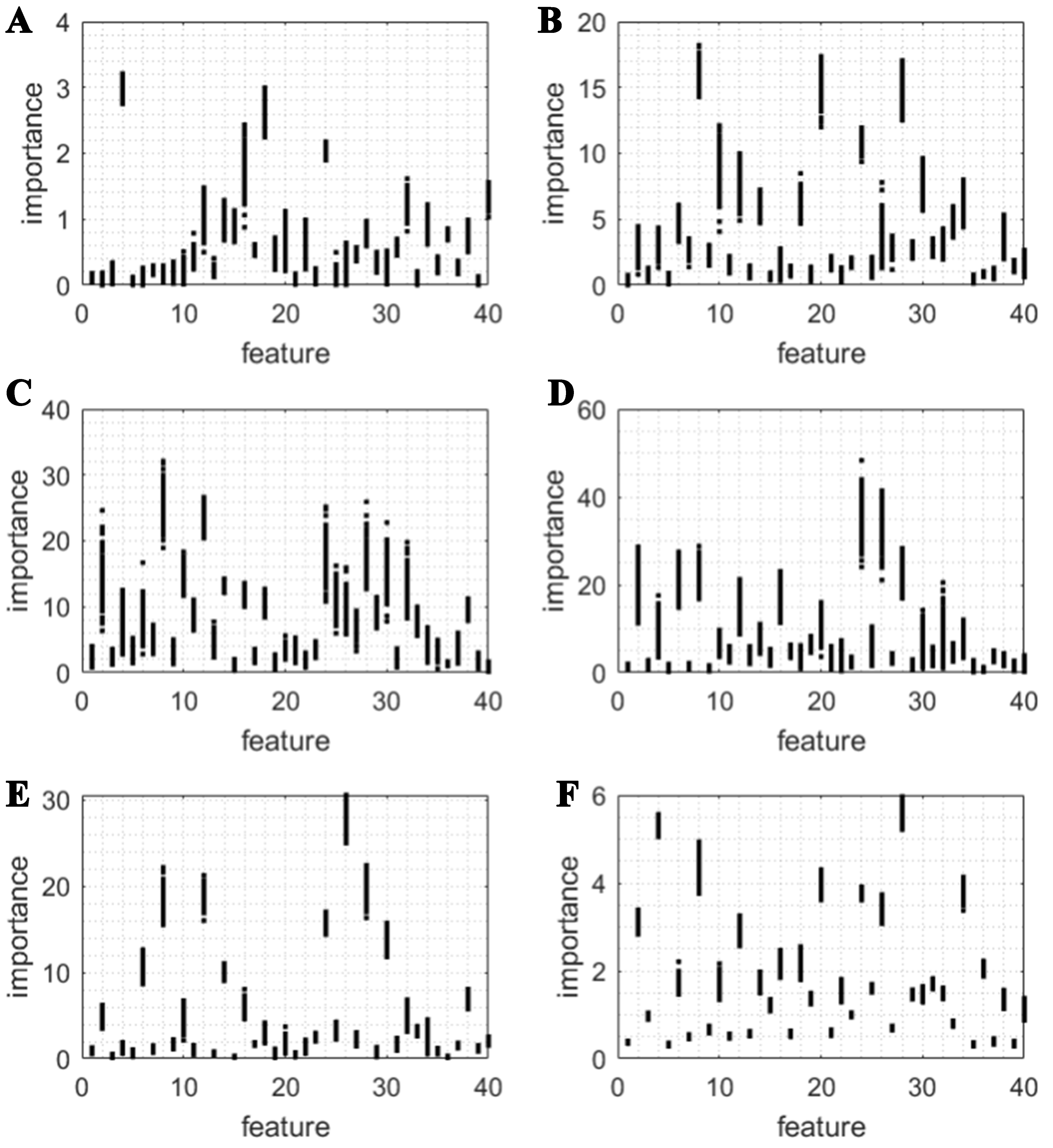
Figure 9. Feature importance in the additive model for (A) Nb alloys, (B) NbI-Nb5Si3 alloys, (C) NbII-Nb5Si3 alloys, (D) SiI-Nb5Si3 alloys, (E) SiII-Nb5Si3 alloys, (F) combined data set. Blue points are for the training, and red points are for the test set. The distribution of vertical points at each feature is over 100 runs differing by random training-test splits.
The following can be concluded from these results. Optimal hyperparameters are quite different among the subsets. This, coupled with data distributions indicating only partially overlapping volumes of sampled space [Figures 2-4], explains difficulties of obtaining a better model by combining the subsets that were also observed with SVR. It might instead be advisable to use separate ML models that are used depending on the type of dataset (a category). The difference between the optimal length parameter (l) corresponds to different roles played by nonlinearity. In particular, GPR-NN reveals that the dependence on the features is practically linear for the Nb alloys dataset [Figure 6], with any noticeable nonlinearity appearing only in
The relative feature importance is different between the datasets. Feature importance is known to be method-dependent. Here it is clearly data-dependent and is different not just between Nb and Nb-Nb5Si3 alloys but also between Nb-Nb5Si3 alloys alloyed at different substitution pair sites. Each vertical set of points in Figure 9 shows the spread of feature importance values over 100 runs differing by random train-test split. The existence of a substantial spread indicates a relatively sparse-data regime, but a relative persistence of relative feature importance with different train-test splits indicates a degree of reliability of ML. Nevertheless, we would caution against reading too much into feature importances obtained with black-box algorithms as they are algorithm-dependent and may return nonsensical results (see Ref.[52] for a spectacular example of significant importance attached by ML to features which are numeric IDs of molecular blocks devoid of any physical meaning).
Importantly, when adding coupling terms [i.e., Equation (6) with increasing N] there is little statistically significant improvement in RMSE of test dataset for any of the subsets or for the combined set [Table 4]. In some of the subsets there was only improvement in the training set error. This indicates that while nonlinearity is important, inter-feature coupling terms are unimportant or non-recoverable probably due to low sampling density in this case.
RMSE of substitution energies (in eV/cell) of alloying elements when using different numbers of terms N in the coupled model of Equation (6)
| Data set | N = 100 | N = 200 | N = 500 | |||
| Training | Test | Training | Test | Training | Test | |
| Nb | 0.17 ± 0.01 | 0.21 ± 0.05 | 0.16 ± 0.02 | 0.22 ± 0.05 | 0.16 ± 0.01 | 0.22 ± 0.06 |
| NbI-Nb5Si3 | 0.13 ± 0.01 | 0.26 ± 0.05 | 0.12 ± 0.01 | 0.25 ± 0.05 | 0.12 ± 0.01 | 0.25 ± 0.05 |
| NbII-Nb5Si3 | 0.11 ± 0.01 | 0.30 ± 0.07 | 0.11 ± 0.01 | 0.35 ± 0.11 | 0.11 ± 0.01 | 0.35 ± 0.13 |
| SiI-Nb5Si3 | 0.24 ± 0.01 | 0.31 ± 0.04 | 0.24 ± 0.01 | 0.31 ± 0.04 | 0.24 ± 0.01 | 0.31 ± 0.04 |
| SiII-Nb5Si3 | 0.09 ± 0.003 | 0.13 ± 0.01 | 0.09 ± 0.003 | 0.13 ± 0.02 | 0.09 ± 0.003 | 0.13 ± 0.01 |
| Combined Nb5Si3 | 0.36 ± 0.004 | 0.52 ± 0.05 | 0.37 ± 0.003 | 0.53 ± 0.04 | 0.38 ± 0.003 | 0.54 ± 0.03 |
Analysis of feature dimensionality reduction
We performed uniform manifold approximation and projection (UMAP) dimensionality reduction of the features and projection of substitution energies predicted via the CE-SVR models on the various datasets [Figure 10]. The UMAP feature analyses show that the two feature vectors after dimensionality reduction were not able to distinguish the target properties unambiguously in most datasets except for Nb and

Figure 10. UMAP feature analyses on various data subsets of substitutions where the substitution energies are predicted by the CE-SVR models: (A) Nb, (B) NbI-Nb5Si3, (C) NbII-Nb5Si3, (D) SiI-Nb5Si3, (E) SiII-Nb5Si3, and (F) combined Nb5Si3. UMAP: Uniform manifold approximation and projection; CE-SVR: center-environment-support vector regression.
CONCLUSIONS
To elucidate fundamental alloying effects of multi-component alloys, it is crucial to develop accurate ML methods to predict the formation energies of Nb and Nb-Nb5Si3 eutectic alloys substituted with various alloying elements in the Nb and Nb5Si3 phases. Various complex factors influence the accuracy of ML prediction. This case study is instructive, in particular, because it presents the problem of ML of materials properties from relatively sparse data often encountered in doped materials systems, and it presents a typical doped system where the data can be naturally divided into subsets based on the type of substitutional site. This allowed us to explore the effect on the quality of ML of using individual data sets for each type of substitution or aggregating data corresponding to different types of substitutional sites. Under sparse data, data combination is typically believed to be promising. We demonstrated here on the example of NbSi alloys that data combination does not necessarily improve the quality of an ML model if the data do not sample similar areas in the feature space. The prediction error for the combined dataset is higher than prediction errors for subsets corresponding to individual different site types. This reflects data distribution, namely that the data from subsets only partially overlap in the feature space and, rather than increasing the density of internal sampling which would facilitate ML, increase the volume of feature space. In this case, it may be recommended to use individual models for the subsets as the perceived advantages of a bigger combined dataset may not be realized. The transferability issues should be paid attention to for doped systems with different substitution configurations.
We also explored the functional form of the dependence of the target property on the features, in particular the roles of nonlinearity and inter-feature coupling. This was possible with the use of GPR-NN hybrid ML method. We showed that while for Nb alloys nonlinearity is unimportant, it is critical to Nb-Nb5Si3 alloys. We find that inter-feature coupling terms are unimportant or non-recoverable, demonstrating the utility of more robust and interpretable additive models for the decoupled feature space. The method allows for estimation of feature importance, although one should not exaggerate the general physical meaning of feature importances during the interpretation of ML models. The relative importance of features can be quite sensitive to detailed local configurations and feature distributions rather than generic to a class of physically similar systems. Overinterpretation should be avoided when one correlates the feature’s importance tightly with its physical significance, as commonly found in the literature.
We hope that this study will be helpful to researchers in designing optimal ML approaches, including dataset augmentation, algorithm optimization, and feature analysis, for ML of materials properties under limited data in solving doping problems for alloys or semiconductors. For example, if it is understood that combining data is not advantageous as different subsets may not increase the density of sampling and have different optimal hyperparameters, complicating rather than facilitating the ML task, this knowledge can then be used to select appropriate methods for such data, such as methods taking into account data hierarchy[25,53]. Once the kind of dependence of the target on the features (linear vs non-linear or coupled vs. uncoupled) is understood, it can also be used to select more appropriate methods (e.g., simple linear regressions or polynomial models instead of complex ML schemes[20]). Moreover, this work suggests that data-driven feature learning becomes increasingly important rather than the optimization of algorithm and parameters alone due to the feature dependent prediction accuracy.
The prediction of energy changes for substitutional elements in alloys serves as a fundamental theoretical approach to guide the design and optimization of alloy compositions. By accurately forecasting energy changes due to substitution, the CE-based ML approach makes it possible to identify stable alloy phases and preferred occupancy for understanding and evaluating alloying effects, inform the selection of appropriate alloying elements, and mitigate the necessity for extensive empirical experimentation.
DECLARATIONS
Authors’ contributions
Made substantial contributions to conception and design of the study and performed data analysis and interpretation: Manzhos, S.; Liu, Y.
Performed data acquisition and provided administrative, technical, and material support: Tang, Y.; Xiao, B.; Liu, Y.
Wrote the manuscript: Tang, Y.; Manzhos, S.; Liu, Y.
Review and editing: Tang, Y.; Manzhos, S.; Liu, Y.; Ihara, M.
Availability of data and materials
The data and code supporting the findings of this study are available at the following URL: https://github.com/Don-sugar/ML_script.
Financial support and sponsorship
Liu, Y.; Tang, Y. and Xiao. B. thank the financial support of the National Natural Science Foundation of China (Nos. 52373227, 52201016, and 91641128) and the National Key R&D Program of China (Nos. 2017YFB0701502 and 2017YFB0702901). This work was also supported by the Shanghai Technical Service Center for Advanced Ceramics Structure Design and Precision Manufacturing (No. 20DZ2294000), and the Shanghai Technical Service Center of Science and Engineering Computing, Shanghai University. The authors acknowledge the Beijing Super Cloud Computing Center, Hefei Advanced Computing Center, and Shanghai University for providing HPC resources. Manzhos, S. and Ihara, M. thank JST Mirai Program, Japan (Grant No. JPMJMI22H1). The grantors had no role in the experiment design, collection, analysis and interpretation of data, and writing of the manuscript.
Conflicts of interest
Manzhos, S. is a member of the Editorial Board of Journal of Materials Informatics, and Liu, Y. is a member of the Youth Editorial Board of the same journal. Liu, Y. also served as a Guest Editor for the special issue titled “Unlocking the AI Future of Materials Science”: Selected Papers from the International Workshop on Data-driven Computational and Theoretical Materials Design (DCTMD). They were not involved in any steps of the editorial processing, notably including reviewer selection, manuscript handling, or decision-making. The other authors declare no conflicts of interest.
Ethical approval and consent to participate
Not applicable.
Consent for publication
Not applicable.
Copyright
© The Author(s) 2025.
Supplementary Materials
REFERENCES
1. Xie, T.; Grossman, J. C. Crystal graph convolutional neural networks for an accurate and interpretable prediction of material properties. Phys. Rev. Lett. 2018, 120, 145301.
2. Ward, L.; Liu, R.; Krishna, A.; et al. Including crystal structure attributes in machine learning models of formation energies via Voronoi tessellations. Phys. Rev. B. 2017, 96, 024104.
3. Wang, T.; Tan, X.; Wei, Y.; Jin, H. Accurate bandgap predictions of solids assisted by machine learning. Mater. Today. Commun. 2021, 29, 102932.
4. Alsalman, M.; Alqahtani, S. M.; Alharbi, F. H. Bandgap energy prediction of senary zincblende III–V semiconductor compounds using machine learning. Mater. Sci. Semicond. Process. 2023, 161, 107461.
5. Li, Y.; Wu, Y.; Han, Y.; et al. Local environment interaction-based machine learning framework for predicting molecular adsorption energy. J. Mater. Inf. 2024, 4, 4.
6. Kohn, W.; Sham, L. J. Self-consistent equations including exchange and correlation effects. Phys. Rev. 1965, 140, A1133-8.
7. Ming, H.; Zhou, Y.; Molokeev, M. S.; et al. Machine-learning-driven discovery of Mn4+-doped red-emitting fluorides with short excited-state lifetime and high efficiency for mini light-emitting diode displays. ACS. Mater. Lett. 2024, 6, 1790-800.
8. Bone, J. M.; Childs, C. M.; Menon, A.; et al. Hierarchical machine learning for high-fidelity 3D printed biopolymers. ACS. Biomater. Sci. Eng. 2020, 6, 7021-31.
9. Zhu, J.; Ding, L.; Sun, G.; Wang, L. Accelerating design of glass substrates by machine learning using small-to-medium datasets. Ceram. Int. 2024, 50, 3018-25.
10. Shim, E.; Tewari, A.; Cernak, T.; Zimmerman, P. M. Machine learning strategies for reaction development: toward the low-data limit. J. Chem. Inf. Model. 2023, 63, 3659-68.
11. Im, J.; Lee, S.; Ko, T.; Kim, H. W.; Hyon, Y.; Chang, H. Identifying Pb-free perovskites for solar cells by machine learning. npj. Comput. Mater. 2019, 5, 177.
12. Yang, J.; Manganaris, P.; Mannodi-Kanakkithodi, A. Discovering novel halide perovskite alloys using multi-fidelity machine learning and genetic algorithm. J. Chem. Phys. 2024, 160, 064114.
13. Liu, C.; Fujita, E.; Katsura, Y.; et al. Machine learning to predict quasicrystals from chemical compositions. Adv. Mater. 2021, 33, 2102507.
14. Isayev, O.; Oses, C.; Toher, C.; Gossett, E.; Curtarolo, S.; Tropsha, A. Universal fragment descriptors for predicting properties of inorganic crystals. Nat. Commun. 2017, 8, 15679.
15. Liu, Y.; Wang, J.; Xiao, B.; Shu, J. Accelerated development of hard high-entropy alloys with data-driven high-throughput experiments. J. Mater. Inf. 2022, 2, 3.
16. Christensen, A. S.; Bratholm, L. A.; Faber, F. A.; Anatole von Lilienfeld, O. FCHL revisited: faster and more accurate quantum machine learning. J. Chem. Phys. 2020, 152, 044107.
17. Bartók, A. P.; Kondor, R.; Csányi, G. On representing chemical environments. Phys. Rev. B. 2013, 87, 184115.
19. Donoho, D. L. High-dimensional data analysis: the curses and blessings of dimensionality. In AMS Conference on Math Challenges of the 21st Century; AMS, 2000. https://dl.icdst.org/pdfs/files/236e636d7629c1a53e6ed4cce1019b6e.pdf. (accessed 16 Jun 2025).
20. Allen, A. E. A.; Tkatchenko, A. Machine learning of material properties: predictive and interpretable multilinear models. Sci. Adv. 2022, 8, eabm7185.
21. Liu, D. D.; Li, Q.; Zhu, Y. J.; et al. High-throughput phase field simulation and machine learning for predicting the breakdown performance of all-organic composites. J. Phys. D. Appl. Phys. 2024, 57, 415502.
22. Rabitz, H.; Aliş, ÖF. General foundations of high-dimensional model representations. J. Math. Chem. 1999, 25, 197-233.
23. Rabitz, H.; Aliş, ÖF.; Shorter, J.; Shim, K. Efficient input - output model representations. Comput. Phys. Commun. 1999, 117, 11-20.
24. Li, G.; Hu, J.; Wang, S. W.; Georgopoulos, P. G.; Schoendorf, J.; Rabitz, H. Random sampling-high dimensional model representation (RS-HDMR) and orthogonality of its different order component functions. J. Phys. Chem. A. 2006, 110, 2474-85.
25. Manzhos, S.; Carrington, T.; Ihara, M. Orders of coupling representations as a versatile framework for machine learning from sparse data in high-dimensional spaces. Artif. Intell. Chem. 2023, 1, 100008.
26. Ren, O.; Boussaidi, M. A.; Voytsekhovsky, D.; Ihara, M.; Manzhos, S. Random sampling high dimensional model representation Gaussian process regression (RS-HDMR-GPR) for representing multidimensional functions with machine-learned lower-dimensional terms allowing insight with a general method. Comput. Phys. Commun. 2022, 271, 108220.
27. Li, G.; Xing, X.; Welsh, W.; Rabitz, H. High dimensional model representation constructed by support vector regression. I. Independent variables with known probability distributions. J. Math. Chem. 2017, 55, 278-303.
28. Chen, H.; Wong, L. L.; Adams, S. SoftBV - a software tool for screening the materials genome of inorganic fast ion conductors. Acta. Crystallogr. B. Struct. Sci. Cryst. Eng. Mater. 2019, 75, 18-33.
29. Wong, L. L.; Phuah, K. C.; Dai, R.; Chen, H.; Chew, W. S.; Adams, S. Bond valence pathway analyzer - an automatic rapid screening tool for fast ion conductors within softBV. Chem. Mater. 2021, 33, 625-41.
30. Li, Y.; Zhu, R.; Wang, Y.; Feng, L.; Liu, Y. Center-environment deep transfer machine learning across crystal structures: from spinel oxides to perovskite oxides. npj. Comput. Mater. 2023, 9, 1068.
31. Perepezko, J. H. Materials science. The hotter the engine, the better. Science 2009, 326, 1068-9.
32. Bewlay, B. P.; Jackson, M. R.; Zhao, J.; Subramanian, P. R.; Mendiratta, M. G.; Lewandowski, J. J. Ultrahigh-temperature Nb-silicide-based composites. MRS. Bull. 2003, 28, 646-53.
33. Shu, J.; Dong, Z.; Zheng, C.; et al. High-throughput experiment-assisted study of the alloying effects on oxidation of Nb-based alloys. Corros. Sci. 2022, 204, 110383.
34. Shi, S.; Zhu, L.; Jia, L.; Zhang, H.; Sun, Z.
35. Xu, W.; Han, J.; Wang, C.; et al. Temperature-dependent mechanical properties of alpha-/beta-Nb5Si3 phases from first-principles calculations. Intermetallics 2014, 46, 72-9.
36. Papadimitriou, I.; Utton, C.; Tsakiropoulos, P. The impact of Ti and temperature on the stability of Nb5Si3 phases: a first-principles study. Sci. Technol. Adv. Mater. 2017, 18, 467-79.
37. Liu, G.; Jia, L.; Kong, B.; Guan, K.; Zhang, H. Artificial neural network application to study quantitative relationship between silicide and fracture toughness of Nb-Si alloys. Mater. Design. 2017, 129, 210-8.
38. Hart, G. L. W.; Mueller, T.; Toher, C.; Curtarolo, S. Machine learning for alloys. Nat. Rev. Mater. 2021, 6, 730-55.
39. Li, Y.; Xiao, B.; Tang, Y.; et al. Center-environment feature model for machine learning study of spinel oxides based on first-principles computations. J. Phys. Chem. C. 2020, 124, 28458-68.
40. Wang, X.; Xiao, B.; Li, Y.; et al. First-principles based machine learning study of oxygen evolution reactions of perovskite oxides using a surface center-environment feature model. Appl. Surf. Sci. 2020, 531, 147323.
41. Tang, Y.; Xiao, B.; Chen, J.; et al. Multi-component alloying effects on the stability and mechanical properties of Nb and Nb–Si alloys: a first-principles study. Metall. Mater. Trans. A. 2023, 54, 450-72.
42. Ouyang, R.; Curtarolo, S.; Ahmetcik, E.; Scheffler, M.; Ghiringhelli, L. M. SISSO: a compressed-sensing method for identifying the best low-dimensional descriptor in an immensity of offered candidates. Phys. Rev. Mater. 2018, 2, 083802.
43. A.A.Baikov Institute of Metallurgy and Materials Science. Database on properties of chemical elements. http://phases.imet-db.ru/elements/mendel.aspx?main=1. (accessed 16 Jun 2025).
44. Ducker, H.; Burges, C. J. C.; Kaufman, L.; Smola, A. J.; Vapnik, V. Support vector regression machines. In Advances in Neural Information Processing Systems. 1996. https://proceedings.neurips.cc/paper_files/paper/1996/file/d38901788c533e8286cb6400b40b386d-Paper.pdf. (accessed 16 Jun 2025).
45. Chang, C. C.; Lin, C. J. LIBSVM: a library for support vector machines. ACM. Trans. Intell. Syst. Technol. 2011, 2, 1-27.
47. Manzhos, S.; Ihara, M. Neural network with optimal neuron activation functions based on additive Gaussian process regression. J. Phys. Chem. A. 2023, 127, 7823-35.
48. Rasmussen, C. E.; Williams, C. K. I. Gaussian processes for machine learning. The MIT Press; 2005. https://gaussianprocess.org/gpml/chapters/RW.pdf. (accessed 16 Jun 2025).
49. Duvenaud, D. K.; Nickisch, H.; Rasmussen, C. E. Additive Gaussian processes. In: Advances in Neural Information Processing Systems. 2011. https://proceedings.neurips.cc/paper_files/paper/2011/file/4c5bde74a8f110656874902f07378009-Paper.pdf. (accessed 16 Jun 2025).
50. Manzhos, S.; Ihara, M. Orders-of-coupling representation achieved with a single neural network with optimal neuron activation functions and without nonlinear parameter optimization. Artif. Intell. Chem. 2023, 1, 100013.
51. Sobol', I. M. On the distribution of points in a cube and the approximate evaluation of integrals. USSR. Comput. Math. Math. Phys. 1967, 7, 86-112.
52. Abarbanel, O. D.; Hutchison, G. R. Machine learning to accelerate screening for Marcus reorganization energies. J. Chem. Phys. 2021, 155, 054106.
Cite This Article
How to Cite
Download Citation
Export Citation File:
Type of Import
Tips on Downloading Citation
Citation Manager File Format
Type of Import
Direct Import: When the Direct Import option is selected (the default state), a dialogue box will give you the option to Save or Open the downloaded citation data. Choosing Open will either launch your citation manager or give you a choice of applications with which to use the metadata. The Save option saves the file locally for later use.
Indirect Import: When the Indirect Import option is selected, the metadata is displayed and may be copied and pasted as needed.
About This Article
Special Issue
Copyright

Data & Comments
Data
0


Comments
Comments must be written in English. Spam, offensive content, impersonation, and private information will not be permitted. If any comment is reported and identified as inappropriate content by OAE staff, the comment will be removed without notice. If you have any queries or need any help, please contact us at [email protected].