


Mapping pareto fronts for efficient multi-objective materials discovery


Abstract
With advancements in automation and high-throughput techniques, we can tackle more complex multi-objective materials discovery problems requiring a higher evaluation budget. Given that experimentation is greatly limited by evaluation budget, maximizing sample efficiency of optimization becomes crucial. We discuss the limitations of using hypervolume as a performance indicator and propose new metrics relevant to materials experimentation: such as the ability to perform well for complex high-dimensional problems, minimizing wastage of evaluations, consistency/robustness of optimization, and ability to scale well to high throughputs. With these metrics, we perform an empirical study of two conceptually different and state-of-the-art algorithms (Bayesian and Evolutionary) on synthetic and real-world datasets. We discuss the merits of both approaches with respect to exploration and exploitation, where fully resolving the Pareto Front provides more knowledge of the best material.
Keywords
INTRODUCTION
Innovation in materials science is being accelerated with machine learning and high-throughput experimentation (HTE) capabilities[1]. Users not only save time on experimentation by virtue of automated workflows with faster processing, but also leverage on equipment with larger batches of experiments to increase throughput and thus minimize experimental time[2]. There have been many successful applications of HTE, particularly in the single objective problem space alongside machine learning-assisted optimization strategies[3-6]. However, many real-world problems are more complex, specifically with multiple conflicting properties to be optimized, for example: strength vs. ductility in metal alloys[7], device thickness vs. fill factor in photovoltaics[8], or selectivity vs. current density in catalysts[9]. In addition, such problems may include constraints that restrict the space of feasible solutions. This drives the need to integrate multi-objective optimization strategies with constraint handling capabilities into the HTE setups[10-12]. The first step could consist of formulating complex material science problems as constrained multi-objective optimization problems (CMOPs).
A CMOP with m objectives and (q + k) constraints can be defined as:
min F(x) = (f1(x), ..., fm(x))T (1)
st gi(x) ≥ 0, i = 1, ..., q
hj(x) = 0, j = 1, ..., k
x ∈ Rn
where F(x) defines the multi-dimensional objectives to be optimized, and gi(x) and hj(x) define the inequality and equality constraints, respectively. A solution x is an n-dimensional vector of decision variables. To determine the objective value of a solution, a Pareto-optimal solution x1 dominates another solution x2 if F(x1) ≤ F(x2) where they are feasible. A total set of all feasible and Pareto-optimal solutions can then be defined as the Pareto Front (PF), which represents all solutions with the optimal trade-off between objectives.
Disovery problem in a HTE platform is usually of combinatorial nature with unexplored regions of objective space, given some mixture of chemicals, precursors, and other process parameters. This problem can be formulated as a CMOP where the target objective space or PF is unexplored, and models trained on existing data must extrapolate to[13-15]. This is achieved through the selection and evaluation of available solutions x ∈ Rn, where each solution represents the set of experimental input parameters (chemicals, temperature settings, etc.) used in the screening. The number of data points is typically low, with most works generally limited to around 102-103 data points due to practical bottlenecks such as time taken to synthesize and characterize, or simply due to a limited time/cost budget.
In addition, the PF can be discontinuous with multiple infeasible regions due to underlying property limitations such as phase boundaries/solubility limits, or engineering rules, for example, summing mixtures to 100%[16]. Such constraints can also be knowledge-based, where a domain expert with prior knowledge sets them to pre-emptively “avoid” poor results and converge faster[17-19]. Figure 1 illustrates an example of such a problem.

Figure 1. Illustration of constrained multi-objectives for a convex minimization problem in bi-objective space. The addition of infeasible regions in grey shifts the original PF from solid red to blue.
CMOPs can be solved in various ways, but recently, two classes of algorithms have shown promise in solving such problems with a high level of success, namely: multi-objective evolutionary algorithms (MOEA) and multi-objective Bayesian optimization (MOBO).
MOEAs[20] work by maintaining and evolving a population of solutions across an optimization run. For example, Genetic Algorithms (GA) are a specific subset that utilizes genetic operators inspired by biological processes: members of the population are selected to become parents based on a specific selection criterion, and then undergo crossover and mutation to form a children population[21]. Within the field of MOEAs, various constraint handling techniques have been proposed[22-24], as well as extensions of MOEAs to many-objective (m > 2) problems[25]. MOEAs are well suited to implementations where solutions can be tested in parallel, given their population-based approach, where each generation’s population can be treated as a batch. MOEAs have been successfully applied in materials-specific multi-objective problems: experimental data is used to construct a machine learning model which is then treated as a computation optimization problem to be solved, and the results evaluated physically[26-28]. The use of MOEAs relevant to materials science has seen computational and inverse design problems as well[29-31].
MOBOs leverage surrogate models to cheaply predict some black-box function, and then use an acquisition function to probabilistically compute a predictive function and return the best possible candidate where the gain is maximized[32]. The choice of surrogate model can depend on the user, but in recent literature, it has become synonymous with ‘kriging’ which refers specifically to the use of Gaussian Processes (GP) as the surrogate model, taking advantage of its flexibility and robustness[33]. The extension of MOBOs to CMOPs is less mature, with relatively new implementations that cover parallelization, multi-objective and constraints[34-36]. On top of these, there are also hybrid variants such as TSEMO[37] or MOEA/D-EGO[38] which integrate the use of MOEAs to improve the prediction quality of the underlying surrogate models. In general, BO as an overarching optimization strategy has already been established as an attractive strategy for use in both computational design problems[39-41] and experimentation problems[42-45] due to its sample efficient approach.
As previously discussed, the PF defines the set of optimal solutions of a CMOP. For optimization of CMOPs, hypervolume (HV) is often used as a performance indicator. It defines the Euclidean distance bounded by a point, and the reference point in a single dimension, and a HV in multiple dimensions. It directly shows the quality of the solutions since a solution set with high HV is closer to the true PF and is diverse as it effectively dominates more objective space. An illustration of the HV measure for a multi-objective (two dimensions for illustration) convex minimization problem is presented in Figure 2, where HV is computed by finding the area of non-dominated solutions, i.e., the solutions closest to PF without any competitor, bounded by a reference point.

Figure 2. Illustration of hypervolume for a convex minimization problem in bi-objective space. The red line represents the ground truth PF, while the blue points and region reflect the best-known solutions and their associated hypervolume, respectively. The green point and region are then used to illustrate the contribution of a newly evaluated solution. The computation of hypervolume in objective space is performed with respect to a lower bound with a reference point, shown by the red star. PF: Pareto Front.
Aside from being a performance metric to compare optimization strategies, HV can also be directly evaluated to guide the convergence of various algorithms. Hanaoka et al. showed that scalarization-based MOBOs may be best suited for clear exploitation and/or preferential optimization trajectory of objectives, whereas HV-based MOBOs are better for exploration of the entire search space[46]. Indeed, HV-based approaches empirically show a preference in proposed solutions towards the extrema of a PF[47,48] and thus can better showcase extrapolation. In contrast, scalarization approaches to reduce multi-objective problems to single-objective ones, such as hierarchically in Chimera[49] or any user-defined function[50], have limitations: (i) it is difficult to determine how to properly scalarize objectives; (ii) single-objective optimization methods cannot propose a set of solutions that explicitly consider the trade-off between objectives.
MATERIALS AND METHODS
Within the context of multi-objective optimization and material science implementation, two state-of-the-art algorithms were compared in the present work: q-Noisy Expected Hypervolume Improvement (qNEHVI)[51] and Unified Non-dominated Sorting Genetic Algorithm III (U-NSGA-III)[52]. They are MOBO and MOEA-based algorithms, respectively, and were chosen based on their reported performance in solving complex CMOPs (with respect to HV score), and the fact that they are capable of highly parallel sampling, making them suitable for integration within an HTE framework. Furthermore, both algorithms are chosen from open-source Python libraries, making them easy to implement and enabling the reproducibility of results presented.
qNEHVI is a HV-based MOBO that utilizes expected HV improvement, which was shown to outperform other state-of-the-art approaches of different means, such as scalarization, entropy-based and even other HV-based approaches like TSEMO. It works by extending the classic Expected Improvement acquisition function[53] to HV as an objective[54], where randomized Quasi-Monte Carlo (QMC) samples from the model posterior are provided for evaluation to maximize acquisition value[55]. Our implementation here relies on the sample code provided by BoTorch for constrained multi-objective optimization, taking both base and raw sampling at 128 (following default settings) to improve computational run times.
U-NSGA-III is an updated implementation of NSGA-III[56,57] to be better generalizable for single and
We thus propose four different metrics.
1. Dimensional contour plots - 10 runs at a relatively large evaluation budget (100 iterations × 8 points per batch) are plotted for the number of dimensions versus total evaluations, colored by HV score. This is done for scalable synthetic problems only and allows us to illustrate performance when dimensionality is scaled up to represent more complex combinatorial problems.
2. Optimization trajectory - a single optimization run at a high evaluation budget (100 iterations × 8 points per batch) is plotted in objective space to illustrate the trajectory of proposed solutions at each iteration towards the PF. This allows us to graphically analyze how either algorithm traverses the objective space or provides a different perspective in understanding the exploration-exploitation trade-off.
3. Probability density map - 10 runs at a lower evaluation budget (24 iterations × 8 points per batch) are plotted all together in objective space and colored according to their probability density function (PDF) value, which is computed via a Gaussian kernel density function (gaussian_kde from SciPy). This is an alternative to optimization trajectory, where we instead consider the consistency and robustness during optimization for different random starts.
4. Batch sizing - various batch sizes are compared using log HV difference to illustrate their HV improvement, and thus illustrate the performance of both algorithms when considering different throughputs, as well as whether more gradual optimization (smaller batches but higher iterations) or vice versa is appropriate.
In all cases, we initialized each optimization run with a Sobol sampling of 2*(variables + 1).
For synthetic benchmarks, we select two-objective scalable problems for comparison, as described in Table 1. The ZDT test suite[59] provides a range of PF shapes, while the MW test suite[60] provides constraints and uniquely shaped PFs to challenge the optimization algorithms. Both test suites rely on a similar construction method for minimization problems: taking a single variable function f1 against a shape function f2 as such:
List and details of synthetic problems
| Name | PF Geometry | n_var | n_obj | n_constr | ref_pt |
| ZDT1 | Convex | Scalable | 2 | 0 | [11, 11] |
| ZDT2 | Concave | ||||
| ZDT3 | Disconnected | ||||
| MW7 | Disconnected (mixed) | 2 | [1.2, 1.2] |
min f1(x) = x1 (2)
min f2(x) = g(x)h(f1(x), g(x))
The single variable function closely resembles certain real-life multi-objective problems where input is to be minimized against some other objective, for example, minimizing process temperature, while achieving a target output[42].
Additionally, we repeated our experiments on real-world multi-objective datasets. An unavoidable issue of empirically benchmarking optimization strategies on real-world problems is that some surrogate model must be used in lieu of a black box where new data is experimentally validated. Alternatively, a candidate selection problem can be used where optimization is limited to only proposing new candidates from a pre-labeled dataset until, eventually, the ‘pool’ of samples is exhausted. The benefit of this method over surrogate-based methods is that only real data from the black box is used, rather than data extrapolated from a model approximating its behavior. However, the candidate selection approach assumes that the existing dataset contains all data points necessary to perfectly represent the search space and true PF. It is generally not possible to prove that this is the case unless the exact function mapping input to output of the black box is known, or the dataset contains all possible combinations of input/output pairs and is therefore a complete representation of the problem like that of inverse design.
Here, due to the relatively small size of the datasets (~102 data points), the candidate selection method was not implemented. Instead, we relied on training an appropriate regressor to model the dataset. The two real-world benchmarks used in this paper are presented in Table 2, with details of implementation in Supplementary Figures 1 and 2. Materials datasets with constraints are hard to find from available HTE literature, asides from simple combinatorial setups that need to sum to 100%. Another example is from Cao et al.[43], which included complex constraints in the form of solubility, although we were unable to attain their full dataset and solubility classifier.
List and details of real-world problems
RESULTS AND DISCUSSION
U-NSGA-III in Figure 3A and C showed a more gradual change in color and did not reach the maximum values for higher dimensions, indicating a slower rate of convergence and poorer HV improvement, respectively, which scale with dimensions. In contrast, results presented in Figure 3B and D for ZDT1 and ZDT2, respectively, indicate that qNEHVI converges fast with greater HV improvement, as illustrated by the bright yellow coloration which appears early and maintains this up to dim = 12 with little loss in initial performance. qNEHVI, while showing superiority in overall HV score for the ZDT3 and MW7 problem, had a lower rate of convergence and maximum HV improvement as dimensions increase, illustrated in Figure 3F and H by the color gradient. Although we note that in other literature, GP models tend to perform poorly at high dimensionalities[63,64], this was not observed here, our results here only consider up to 12 dimensions.
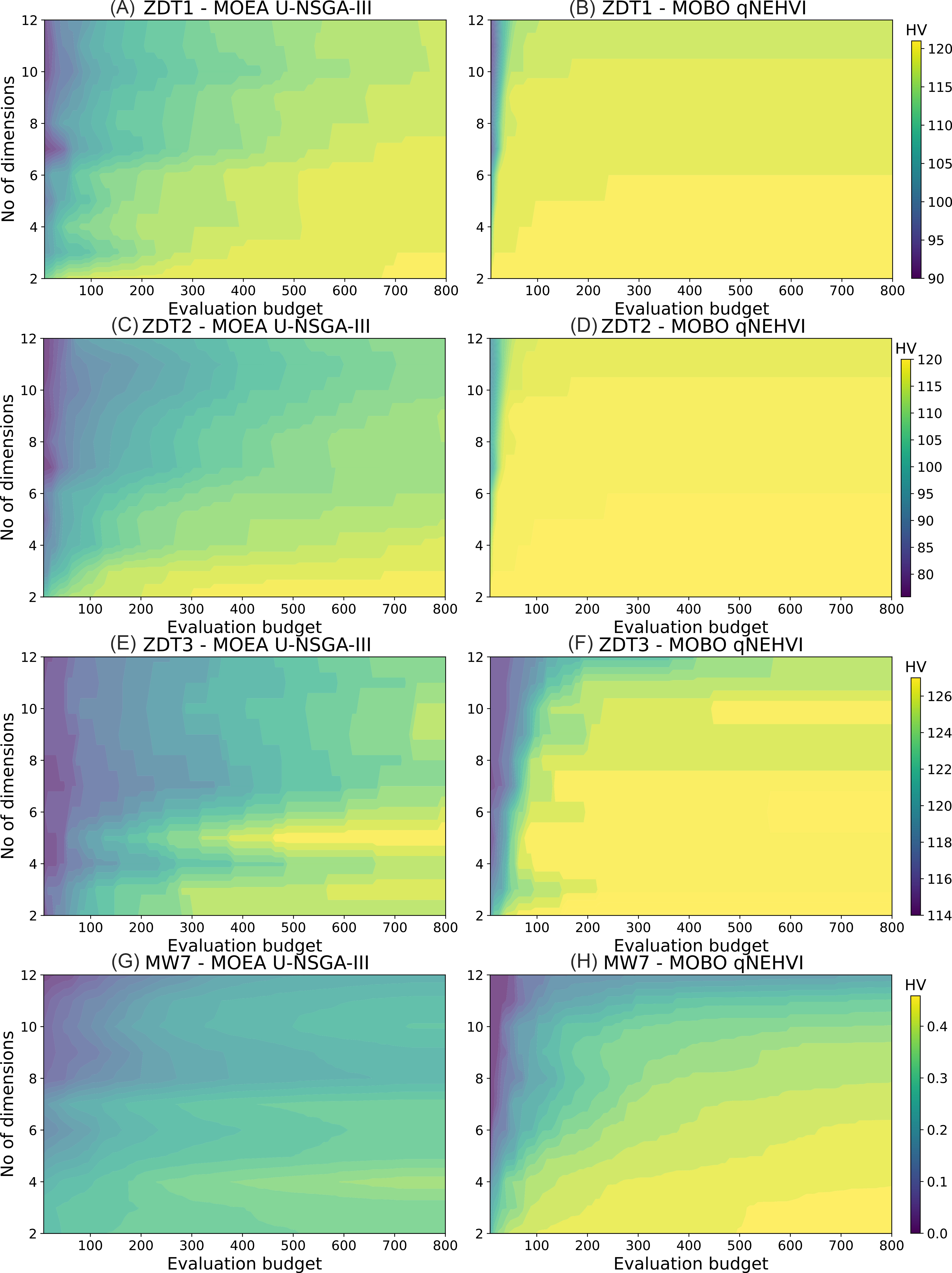
Figure 3. Contour plots for dimension vs evaluation budget. (A and B) ZDT1; (Cand D) ZDT2; (E and F) ZDT3; (G and H) MW7. The color bar illustrates the mean cumulative HV score with respect to cumulative evaluations, over a total evaluation budget of 100 iterations × 8 points per batch. Results are averaged over only 5 runs due to the high computational cost of searching over many dimensions. The results here show that qNEHVI is a far superior method when looking at only HV as a performance metric. HV: hypervolume; MOBO: multi-objective Bayesian optimization; MOEA: multi-objective evolutionary algorithms; qNEHVI: q-Noisy Expected Hypervolume Improvement; U-NSGA-III: Unified Non-dominated Sorting Genetic Algorithm III.
It should be noted that in Figure 3E, U-NSGA-III’s HV score on the ZDT3 problem scales inconsistently with dimensionality: dim = 5 shows better HV improvement (brighter color) compared to dim = 2 to 4. We attribute this to the disconnected PF being strongly affected by differences in initialization, where entire regions can be lost as the evolutionary process fails to extrapolate and explore sufficiently. Lastly, we observe in Figure 3G for MW7 that U-NSGA-III performs significantly worst as compared to qNEHVI, regardless of dimensionality. The presence of more complex constraints in the problem means that many solutions are likely to be infeasible and require more iterations to evolve to feasibility according to the evolution mechanism. Infeasible solutions do not contribute to HV improvement at all, and we note that this is one of the limitations of plotting using HV as a metric, where feasibility management is not clearly reflected.
In order to investigate why qNEHVI presented a greater HV improvement for qNEHVI, we then proceeded to plot the optimization trajectory to observe solutions in objective space, as shown in Figure 4. We set the number of dimensions to 8. This is representative of a range of experimental parameters that materials scientists would consider practical. We first performed a single run of 100 iterations × 8 points per batch. The evaluated solutions are plotted onto the objective space and colored by their respective iteration from dark to bright.

Figure 4. Optimization trajectory in objective space for a single run of 100 iterations × 8 points per batch. (A and B) ZDT1; (C and D) ZDT2; (E and F) ZDT3; (G and H) MW7. The red line represents the true PF, while MW7 being a constrained problem has an additional blue line to show the unconstrained PF. The color of each experiment refers to the number of iterations. All problems clearly show a more gradual evolution of results as the number of iterations progresses in U-NSGA-III, whereas qNEHVI rapidly approaches PF and then fails to converge further. HV: hypervolume; MOBO: multi-objective Bayesian optimization; MOEA: multi-objective evolutionary algorithms; qNEHVI: q-Noisy Expected Hypervolume Improvement; U-NSGA-III: Unified Non-dominated Sorting Genetic Algorithm III.
The general observations in Figure 4A-H comparing qNEHVI to U-NSGA-III are consistent with results previously reported in Figure 3, specifically in terms of HV scores and convergence rate. In all subfigures, qNEHVI was able to propose solutions at the PF within the first 20 iterations, as shown by the darker color of points along the red line (true PF). This suggests that it is very sample efficient. However, it was unable to fully exploit the region of objective space close to the PF, and solutions in later iterations are non-optimal. In fact, in Figure 4B and D, ZDT1 and ZDT2, respectively, a large portion of solutions lie along the f1 = x1 = 0 line. This is explained by the choice of reference point, which we explore in more detail in Supplementary Figures 3 and 4.
We hypothesize that qNEHVI is unable to identify multiple bi-objective points along the PF because the underlying GP surrogate model did not accurately model the PF for ZDT1-3. As for MW7, despite the algorithm being able to propose many solutions near the unconstrained PF, it failed to overcome the constraints, as seen by the failure to adjust to the new dotted red line. Similarly, qNEHVI’s superior HV score could be attributed to the stochasticity of QMC sampling providing good solutions, rather than accurate model predictions. This hypothesis is supported by results reported in Supplementary Figure 5, where it can be observed that the GP model did not fully learn the objective function.
In contrast, U-NSGA-III, while requiring a significantly larger number of iterations to reach the PF, had a more consistent optimization trajectory towards the PF, as seen by the gradual color gradient in Figure 4A, C, E, and G. This suggests that there are fewer wasted evaluations for MOEAs, as the latter iterations are targeted towards the PF. However, despite having more solutions near the PF, the HV score is lower for
Notably, we observe in Figure 4E and G that the disconnected PFs for ZDT3 and MW7 can lead to entire regions of objective space being omitted. This is clearly seen in both subfigures where solutions only have a single trajectory towards the nearest PF region. We previously made the statement, based on results reported in Figure 3C and D, for the same synthetic problems, that the disconnected spaces are strongly influenced by initialization, where U-NSGA-III’s mechanism of tournament selection rewards immediate gain over coverage, i.e. exploitation over exploration. This is both a strength and weakness of U-NSGA-III in comparison to qNEHVI, where QMC sampling enables greater exploration of the overall search space as it attempts to maximize coverage across the entire objective space, but not the PF.
Results reported in Figure 5 further reinforce the observation that qNEHVI produces a large pool of non-optimal solutions for all benchmark problems, where many points exist away from the PF. Additionally, the darker coloration for qNEHVI in Figure 5B, D, F and H indicates a much lower probability of occurrence, which reinforces our hypothesis that HV improvement can be partially attributed to QMC sampling. Additionally, Figure 5B and D for ZDT1 and ZDT2, respectively, also show that there were many solutions being proposed at the extrema of f1 = x1.
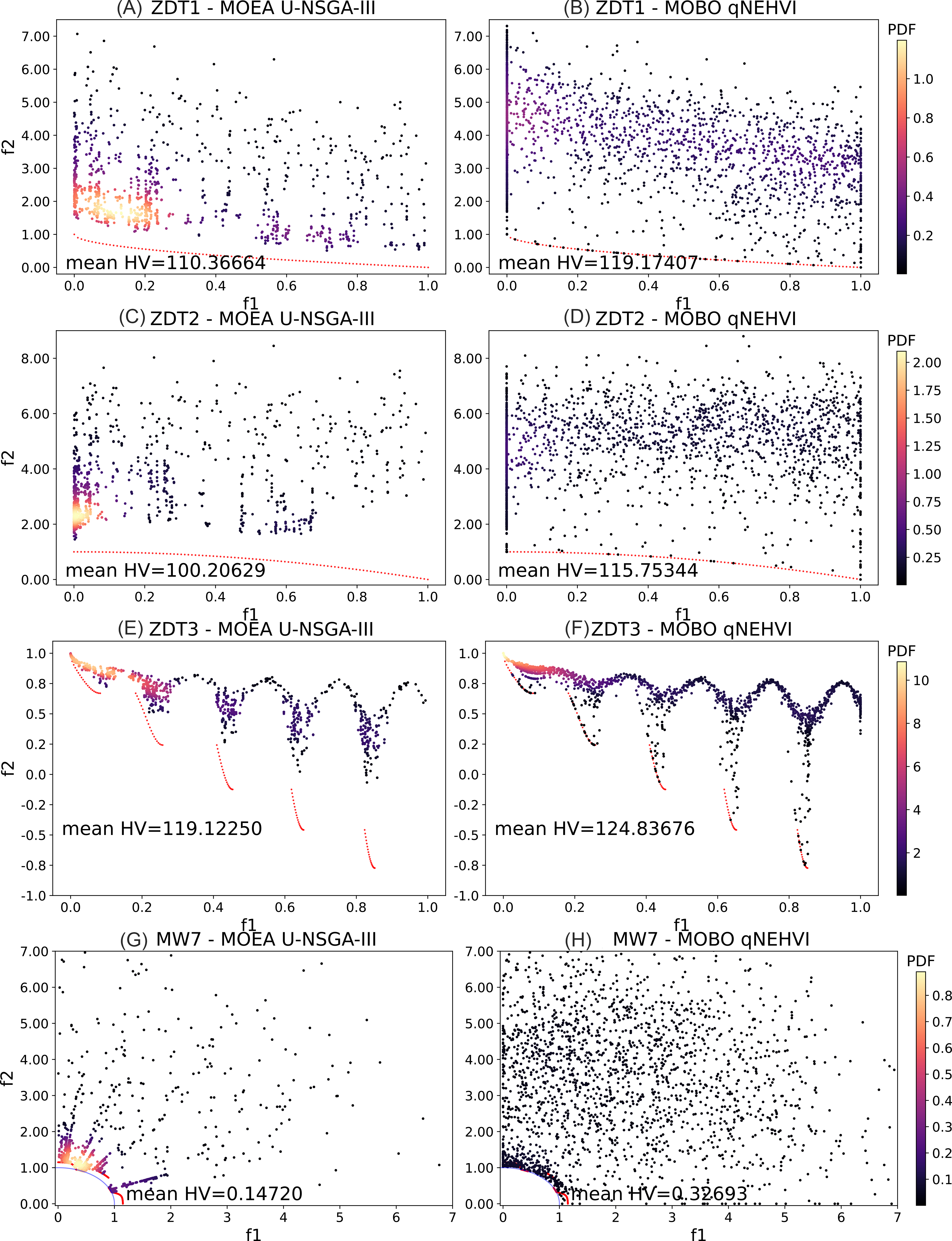
Figure 5. Probability density maps in objective space for 10 runs of 24 iterations × 8 points per batch. (A and B) ZDT1; (C and D) ZDT2; (E and F) ZDT3; (G and H) MW7. The evaluated data points are plotted with a Gaussian kernel density estimate using SciPy to illustrate the distribution of points across objective space. The color bar represents the numerical value of probability density. Results are averaged over the 10 runs and highlight the lower diversity of points and consistency in optimization trajectory for qNEHVI compared to U-NSGA-III. HV: hypervolume; MOBO: multi-objective Bayesian optimization; MOEA: multi-objective evolutionary algorithms; qNEHVI: q-Noisy Expected Hypervolume Improvement; U-NSGA-III: Unified Non-dominated Sorting Genetic Algorithm III.
This is the same behavior as that observed for a single run in Figure 4B and D, and we further elaborate upon it in Supplementary Figure 5. In contrast, the heuristic nature of U-NSGA-III provides more consistency between runs, since selection pressure will always ensure the same set of best parents, as shown by the brighter regions of points near the PF in Figure 5A, C, E and G indicating a higher probability density. Notably, the bright regions are not spread across objective space evenly. There appears to be a preference for the lower range of f1 = x1, i.e. it is simple to derive improvement by simply decreasing x1. This is in line with our previous discussions based on results reported in Figure 4, where U-NSGA-III prefers solutions with immediate improvement. Furthermore, we observe that the bright regions are concentrated near the PF, which indicates that U-NSGA-III was able to consistently approach the PF and maintain a larger pool of near-Pareto solutions over various runs, despite the limited evaluation budget.
In contrast, qNEHVI had relatively few points, although they are lying directly on the PF, which is then shown as a higher mean HV compared to U-NSGA-III. In a real-world context, the larger pool of near-Pareto solutions could have scientific value, especially for users looking to build a materials library and further understand the PF. However, this is not reflected by the HV performance indicator.
The choice of batch size is another important parameter to consider for materials scientists. It can be tuned when attempting to scale up for HTE. A larger batch size is usually ideal since it provides higher throughput and, thus, more time savings since lesser iterations are required. We thus perform optimization on the same synthetic problems for different batch sizes, keeping dimensionality at dim = 8 and with the same evaluation budget of 192 points and 10 runs, as mentioned earlier.
The authors of qNEHVI hypothesized that it operates better at small batch sizes by providing a smoother gradient descent in sequential optimization. Results reported in Figure 6A, B and D for ZDT1, ZDT2 and MW7, respectively, support this hypothesis, and we clearly observe that the lowest batch size setting of 2, as represented by the pink line, has the best performance overall. Interestingly, this is also the case for U-NSGA-III, where the minimum batch size of 2 tends to give better HV for ZDT1-3, as seen by the blue line. This is also empirically shown in literature where, given a total budget, higher populations may impede convergence as it effectively limits the number of iterations[65-67]. Our observations suggest that larger batch sampling may lead to non-optimal candidate solutions being evaluated, especially when the model presents high uncertainty and/or poor accuracy where only a few candidates from the model posterior return a high acquisition value.

Figure 6. Convergence at different batch sizes with the same total evaluation budget of 24 × 8. (A) ZDT1; (B) ZDT2; (C) ZDT3; (D) MW7. We omitted qNEHVI for a batch of 16 due to the prohibitively high computation cost when scaling up. Plots are taken with mean and 95% confidence interval of log10(HVmax - HVcurrent), with HVmax being computed from known PF in pymoo. We follow the same details as for Figure 5. Results suggest that qNEHVI works better with low batching on disconnected PF. HV: hypervolume; PF: Pareto Front; qNEHVI: q-Noisy Expected Hypervolume Improvement; U-NSGA-III: Unified Non-dominated Sorting Genetic Algorithm III.
It is suggested that the same did not apply for MW7 since the disconnected PF was often not fully explored due to differences in initialization, which we discussed previously for Figures 4 and 5. Instead, a larger batch size, i.e., a larger population, is beneficial in learning all disconnected regions of objective space, as seen by the red line in Figure 6D. We also explain why this did not apply to ZDT3: since the initial sampling was generally able to cover the search space well, there are relatively few “lost” regions, as seen in Figure 4C. Additionally, we provide optimization trajectory plots for U-NSGA-III at different batch sizes in Supplementary Figure 6 to illustrate this.
Furthermore, we also observe that qNEHVI has greater variance in log HV difference compared to U-NSGA-III. This further reinforces our hypothesis that the performance of qNEHVI is in part due to the stochastic QMC sampling, while the heuristic nature of U-NSGA-III means that the evolution of solutions is more consistent.
Figure 7 further supports our conclusions drawn from the results reported in Figure 4. As seen in Figure 7B and D, qNEHVI is highly sample efficient, with points at or near the PF within the first 20 iterations or so, indicated by the darker points lying on the red line. However, qNEHVI shows a large random distribution of non-optimal points away from PF across the entire run, as seen by both dark and bright points. U-NSGA-III performs a gradual evolution of points towards the PF, as seen in Figure 7A and C, as well as maintaining a large pool of near-optimal solutions. This is reflected by the lower HV scores for U-NSGA-III compared to those of qNEHVI.
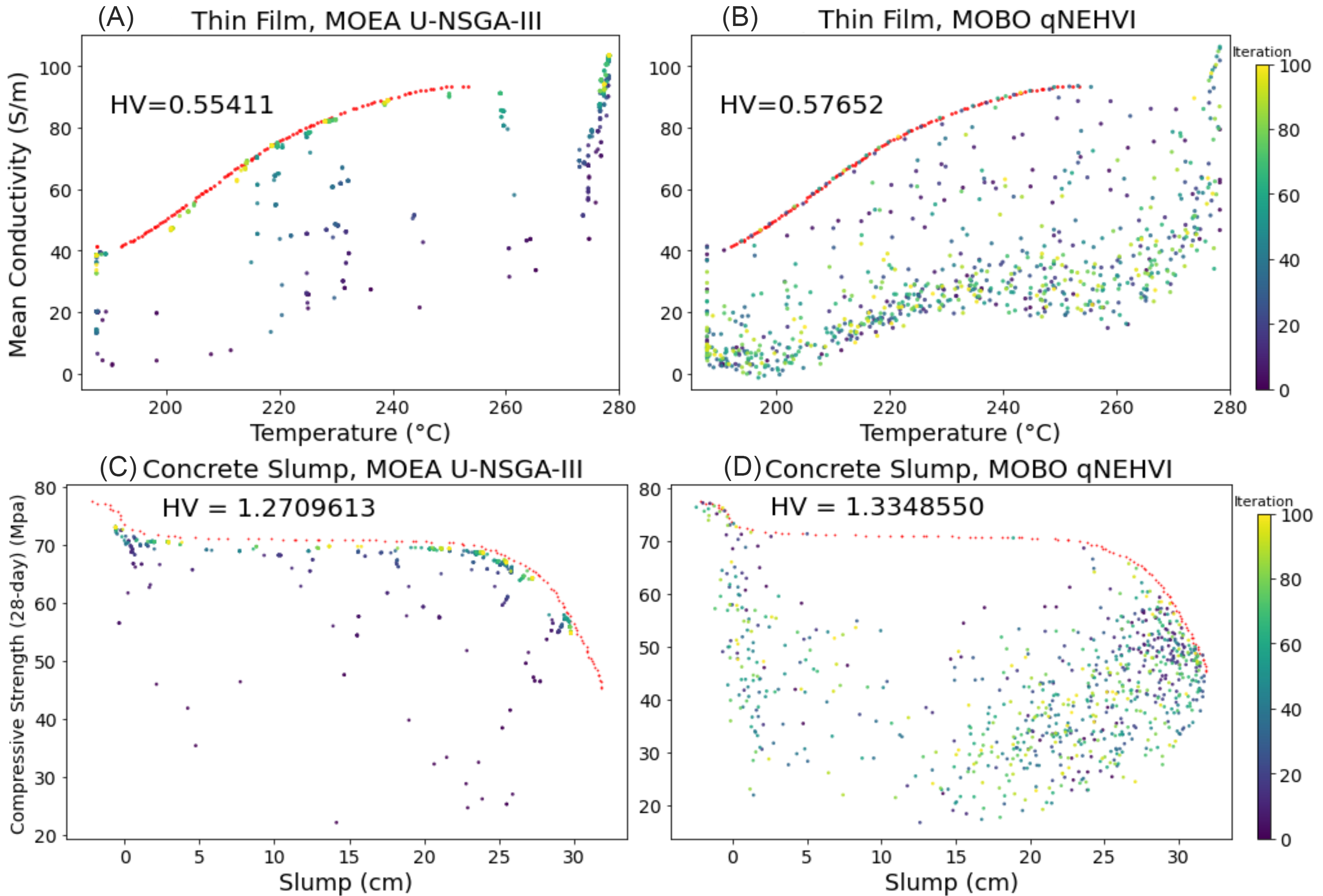
Figure 7. Optimization trajectory in objective space for a single run of 100 iterations × 8 points per batch. (A and B) Thin Film; (C and D) Concrete Slump. Across objective space for a single run of 100 iterations × 8 points per batch. The red line represents the PF. PFs for real-world datasets were virtually generated using NSGA-II for 500 generations with a population size of 100. The color of each experiment refers to the number of iterations. The results here corroborate the “wastage” of solutions in qNEHVI, although which algorithm is superior appears to be problem dependent. HV: hypervolume; MOBO: multi-objective Bayesian optimization; MOEA: multi-objective evolutionary algorithms; PF: Pareto Front; qNEHVI: q-Noisy Expected Hypervolume Improvement; U-NSGA-III: Unified Non-dominated Sorting Genetic Algorithm III.
At a smaller evaluation budget, we observe that U-NSGA-III consistently maintains a large pool of near-optimal solutions, as the bright region is seen nearer to the PF, while reporting a lower mean HV compared to qNEHVI in Figure 8A and E. Figure 8B for the Thin Film problem also corroborates our findings that qNEHVI proposes many non-optimal solutions, as seen by the bright region away from PF, which indicates a higher probability of occurrence.

Figure 8. Probability density maps in objective space for 10 runs of 24 iterations × 8 points per batch. (A and B) Thin film; (C and D) concrete slump. The evaluated data points are plotted with a Gaussian kernel density estimate using SciPy to illustrate the distribution of points across objective space, with a color bar to represent the numerical value of probability density. Results are averaged over 10 runs, taking a smaller evaluation budget of 24 iterations × 8 points = 192. The results here reinforce the finding that qNEHVI has a more random distribution of points, but still outperforms U-NSGA-III for a low evaluation budget. HV: hypervolume; MOBO: multi-objective Bayesian optimization; MOEA: multi-objective evolutionary algorithms; U-NSGA-III: Unified Non-dominated Sorting Genetic Algorithm III.
Interestingly, in Figure 8D for Concrete Slump problem, we observe that qNEHVI is consistently converging to a specific region in objective space, while in Figure 8C, the U-NSGA-III search follows that of Figure 8B with the concentration of solutions at the near-optimal region close to PF. We hypothesize that qNEHVI’s performance for this problem is influenced by how the underlying GP surrogate model learns the function and strongly biases solutions to that specific region. We show further proof in Supplementary Figure 5, where we illustrate the expected PF given by the GP surrogate model.
In contrast, both problems here indicated that U-NSGA-III benefited more from larger batch sizes, as seen by the green line, which is different from what we observed in Figure 6 for synthetic problems. Our hypothesis is that the modeled datasets present a more mathematically difficult optimization problem, with various “obstacles” that inhibit the evolution of solutions towards the PF. We support this by referring to our discussions for Figure 7C and D on Concrete Slump regarding local optima, as well as observing a notable blank region of objective space which U-NSGA-III fails to flesh out in Figure 7A for Thin Film problem. Overall, the results reported here suggest that given state-of-the-art implementations in HT experiments, a small batch size with MOBO is the right strategy to converge rapidly.
Finally, we also studied the effect of batch size on convergence in Figure 9. Results present both similarities and differences with what we observe for synthetic benchmarks in Figure 6. A smaller batch size in qNEHVI was better for both problems, as seen by the purple line, which is consistent with our findings for Figure 6.

Figure 9. Convergence at different batch sizes with the same total evaluation budget of 24 × 8. (A) Thin film; (B) concrete slump. We omitted qNEHVI for a batch of 16 due to the prohibitively high computation cost when scaling up. Plots are taken with mean and 95% confidence interval of log10(HVmax - HVcurrent), with HVmax being computed from known PF in pymoo. The results shown here support our conclusions for qNEHVI in Figure 6 but have marked differences for U-NSGA-III. HV: hypervolume; PF: Pareto Front; qNEHVI: q-Noisy Expected Hypervolume Improvement; U-NSGA-III: Unified Non-dominated Sorting Genetic Algorithm III.
Further discussion
We have compared qNEHVI and U-NSGA-III using both synthetic and real-world benchmarks, considering experimental parameters such as dimensionality and batch size, which materials scientists may face when implementing optimization. Our results suggest that qNEHVI is comparatively more sample efficient in arriving at the PF to maximize HV gain but fails to exploit it. In contrast, we report that U-NSGA-III has a consistent optimization trajectory, and better exploits the PF while maintaining more near-optimal solutions, but only if there are sufficient evaluations to do so. Materials experimentation is usually limited to < 100 evaluations due to physical constraints such as time/material depletion. We chose a larger evaluation budget of 192 as we observed that U-NSGA-III was unable to converge to the PF within 100 evaluations, making analysis of results difficult when discussing exploration/exploitation at the PF. Thus, MOEAs may be considered when improvements in automated high-throughput setups enable larger evaluation budgets of ~103 or more. For example, Jiang et al.[68] recently demonstrated seed-mediated synthesis of nanoparticles with ~1,000 experiments. We thus make a case for MOEAs for materials experimentation besides computational design. We present in Table 3 a summary of our discussion.
Summary of both algorithms
| BO - qNEHVI | EA - U-NSGA-III | |
| Features | Stochastic candidates are selected to maximize HV improvement predicted by the GP surrogate model | Tournament selection is incorporated to increase selection pressure, where parents are selected based on reference vectors to maximize diversity and exploitation on the PF |
| Advantages | - Sample efficiency to reach PF - Converges rapidly for up to 10 dimensions | - Maintains good diversity along PF - Computationally cheap |
| Disadvantages | - Computationally expensive, scales poorly to a higher number of objectives - Poor exploitation of PF (high wastage of evaluations) | - Slow convergence that scales with dimensionality |
| Choice of Experiments | - Works well for limited evaluation budgets of < 100 with small (2-4) batch sizes | - Works well for short experimental run times with large evaluation budgets with large batch sizes (6 and above) |
We also argue that such implementations would be best when the objective space is mildly discontinuous (such as structural problems in alloys) since small changes in inputs can cause outputs to vary wildly in objective space, where an evolutionary-based strategy can navigate with better granularity. This is consistent with work by Liang et al.[69] on single-objective problems, which noted that having “multiple well-performing candidates allows one to not only observe regions in design space that frequently yield high-performing samples but also have backup options for further evaluation should the most optimal candidate fail in subsequent evaluations”.
MOEAs also scale better in terms of computational cost[70] as they perform simple calculations to select/recombine/mutate. In comparison, MOBOs train surrogate models and compute acquisition values which are orders of magnitude more expensive compared to EA. Depending on the experiment setup, the ML component may not be able to leverage powerful cluster computing for computationally intensive problems/models. In scenarios where the physical experiment time (synthesis and characterization) is sufficiently short, MOEAs with lower computation overhead, such as U-NSGA-III, could be a better choice to eliminate dead time. We include in Supplementary Table 1 a breakdown of the computing times for both algorithms at different batch sizes.
The choice of batch size to balance optimization performance while minimizing experimental cycles is also important. Empirically, our results obtained suggest that a smaller batch size of around 4 is ideal for the limited evaluation budget of 192 points, although larger batch sizes are preferred for more complex problems (with added difficulty from disconnected regions in objective space, or perhaps the presence of local optima).
A caveat of our work here is that the synthetic problems we chose are a generalization of bi-objective spaces with specific PF geometries that may not translate well for real-life experimentation, especially for many-objective (M > 3) problems. Existing publications for applying optimization to materials discovery generally have no more than 3 objectives. The practicality of optimizing problems with > 3 objectives is still questionable due to the difficulty of defining non-dominance[71], making it difficult to find the PF. Furthermore, the computational cost for hypervolume scales super-polynomially which makes it impractical for optimization. In the source publication for qNEHVI (under supplementary H.8)[51], the authors demonstrate that their implementation is the first to practically implement HV-based optimization up to 5 objectives. We also refer to Tables 8 and 9 in the source publication for NSGA-III[56], which studies its performance for scaling the number of objectives, up to 10. We include results for 3-objective optimization on DTLZ2 under Supplementary Figure 7.
Newer benchmarks with greater difficulties and complex geometries/PFs are tailored towards challenging MOEAs with massive evaluation budgets of up to 107 total observations. An example would be MW5 from the MW test suite, which has narrow tunnel-like feasible regions that are practically impossible for GPs to model, resulting in MOBOs failing to converge. Such benchmarks are unsuitable for drawing conclusions for materials optimization as they assume much larger evaluation budgets of up to 107 observations, and the objective spaces may be unrealistic.Indeed, Epps et al.[45] noted that it is “difficult to impose complex structure on the GPs, which often simply encode continuity, smoothness, or periodicity”.
Furthermore, materials experimentation is usually afflicted with real-world imperfections and deviations during synthesis, or uncertainty due to characterization equipment resolution. For example, MacLeod et al. noted that “the tendency of drop-casted samples to exhibit a wide range of downwards deviations in the apparent conductivity due to the poor sample morphology”[42]. The effect of noise causes deviations in objective values from the “true” ground truth, and although unclear, it is an unavoidable aspect of optimization and should be tackled[72,73]. In Supplementary Figure 8, we perform a comparison of qNEHVI and U-NSGA-III on varying amounts of white noise on outputs.
We also highlight that optimization of both continuous and categorical variables is necessary to unlock a wider decision space for materials discovery, such as when choosing between different catalysts or different synthesis routes towards a desired product. Molecules could have similar physical, chemical, and structural properties within classes/groups/types, and it would be productive to leverage this information as categorical variables. For example, hybrid inorganic-organic perovskites[74] could have different permutations of cations and anions, which report different descriptors. Inorganics incorporate atomic information like electron affinity and electronegativity, while organics could include geometric and electronic information such as molecular weight or dipole moment.
Many high-throughput setups such as flow reactors, specifically leverage only continuous inputs[43]. If categorical variables necessarily need to be considered, a possible approach would be to encode categorical variables into numerical quantities. However, this may lead to information loss since the relationship between different categories is not explicitly encapsulated. We refer to the work by Hase et al.[75] for such an algorithm that maps categorical variables to a continuous latent space and can incorporate relevance weights for each descriptor to the respective variables.
CONCLUSIONS
In conclusion, our results illustrate that existing performance metrics such as HV may not really reflect the goal of fleshing out the PF region. This reflects an aspect of optimization that might be neglected in the purview of multi-objective materials discovery: which is to identify the entire set of optimal solutions that can adequately convey the trade-offs between conflicting objectives for scientific understanding. We thus present alternative illustrative means, such as probability density maps, to better benchmark the performance of optimization strategies for such purposes. We performed an empirical study of two conceptually different optimizers, qNEHVI and U-NSGA-III, using our proposed metrics by which to analyze their performance. Through this, we derive certain conclusions that help us better understand the mechanisms by which constrained multi-objective optimization occurs. Moving ahead, we hope that this can spur further improvement for MOBOs as well as a stronger consideration for the use of MOEAs for materials problems in exploiting the PF.
DECLARATIONS
Authors’ contributionsConceived the research: Low AKY, Hippalgaonkar K
Developed and tested the algorithms and datasets, with key intellectual contributions from all authors: Low AKY, Vissol-Gaudin E, Lim YF
Wrote the manuscript with input from all co-authors: Low AKY
Availability of data and materialsThe source code for our work can be found at https://github.com/Kedar-Materials-by-Design-Lab. A supplementary document is also available.
Financial support and sponsorshipThe authors acknowledge funding from AME Programmatic Funds by the Agency for Science, Technology and Research under Grant (No. A1898b0043) and Grant (No. A20G9b0135). Hippalgaonkar K also acknowledges funding from the NRF Fellowship (NRF-NRFF13-2021-0011).
Conflicts of interestHippalgaonkar K owns equity in a startup focused on applying Machine Learning for Materials.
Ethical approval and consent to participateNot applicable.
Consent for publicationNot applicable.
Copyright© The Author(s) 2023.
Supplementary MaterialsREFERENCES
1. Correa-Baena J, Hippalgaonkar K, van Duren J, et al. Accelerating materials development via automation, machine learning, and high-performance computing. Joule 2018;2:1410-20.
2. Mennen SM, Alhambra C, Allen CL, et al. The evolution of high-throughput experimentation in pharmaceutical development and perspectives on the future. Org Process Res Dev 2019;23:1213-42.
4. Langner S, Häse F, Perea JD, et al. Beyond ternary OPV: high-throughput experimentation and self-driving laboratories optimize multicomponent systems. Adv Mater 2020;32:e1907801.
5. Bash D, Chenardy FH, Ren Z, et al. Accelerated automated screening of viscous graphene suspensions with various surfactants for optimal electrical conductivity. Digit Discov 2022;1:139-46.
6. Mekki-Berrada F, Ren Z, Huang T, et al. Two-step machine learning enables optimized nanoparticle synthesis. NPJ Comput Mater 2021:7.
7. Li Z, Pradeep KG, Deng Y, Raabe D, Tasan CC. Metastable high-entropy dual-phase alloys overcome the strength-ductility trade-off. Nature 2016;534:227-30.
8. Ramirez I, Causa' M, Zhong Y, Banerji N, Riede M. Key tradeoffs limiting the performance of organic photovoltaics. Adv Energy Mater 2018;8:1703551.
9. Ren S, Joulié D, Salvatore D, et al. Molecular electrocatalysts can mediate fast, selective CO2 reduction in a flow cell. Science 2019;365:367-9.
10. Bash D, Cai Y, Chellappan V, et al. Machine learning and high-throughput robust design of P3HT-CNT composite thin films for high electrical conductivity. arXiv preprint 2020;[Accepted]:2011.10382.
11. Grizou J, Points LJ, Sharma A, Cronin L. A curious formulation robot enables the discovery of a novel protocell behavior. Sci Adv 2020;6:eaay4237.
12. Abdel-Latif K, Epps RW, Bateni F, Han S, Reyes KG, Abolhasani M. Self-driven multistep quantum dot synthesis enabled by autonomous robotic experimentation in flow. Adv Intell Syst 2021;3:2000245.
13. Yong W, Zhang H, Fu H, Zhu Y, He J, Xie J. Improving prediction accuracy of high-performance materials via modified machine learning strategy. Comput Mater Sci 2022;204:111181.
14. Lim YF, Ng CK, Vaitesswar U, Hippalgaonkar K. Extrapolative bayesian optimization with gaussian process and neural network ensemble surrogate models. Adv Intell Syst 2021;3:2100101.
15. Klein A, Bartels S, Falkner S, Hennig P, Hutter F. Towards efficient Bayesian optimization for big data. Available from: https://bayesopt.github.io/papers/2015/klein.pdf [Last accessed on 21 Apr 2023].
16. Gopakumar AM, Balachandran PV, Xue D, Gubernatis JE, Lookman T. Multi-objective optimization for materials discovery via adaptive design. Sci Rep 2018;8:3738.
17. Niculescu RS, Mitchell TM, Rao RB, Bennett KP, Parrado-Hernández E. Bayesian network learning with parameter constraints. Available from: https://www.jmlr.org/papers/volume7/niculescu06a/niculescu06a.pdf [Last accessed on 21 Apr 2023].
18. Asvatourian V, Leray P, Michiels S, Lanoy E. Integrating expert’s knowledge constraint of time dependent exposures in structure learning for Bayesian networks. Artif Intell Med 2020;107:101874.
19. Liu Z, Rolston N, Flick AC, et al. Machine learning with knowledge constraints for process optimization of open-air perovskite solar cell manufacturing. Joule 2022;6:834-49.
20. Deb K. Multi-objective optimisation using evolutionary algorithms: an introduction. In: Multi-Objective Evolutionary Optimisation for Product Design and Manufacturing. Springer; 2011:3-34.
22. Fan Z, Li W, Cai X, et al. An improved epsilon constraint-handling method in MOEA/D for CMOPs with large infeasible regions. Soft Comput 2019;23:12491-510.
23. Xu B, Zhang Z. Constrained optimization based on ensemble differential evolution and two-level-based epsilon method. IEEE Access 2020;8:213981-97.
24. Tian Y, Zhang Y, Su Y, Zhang X, Tan KC, Jin Y. Balancing objective optimization and constraint satisfaction in constrained evolutionary multiobjective optimization. IEEE Trans Cybern 2022;52:9559-72.
25. Li B, Li J, Tang K, Yao X. Many-objective evolutionary algorithms: a survey. ACM Comput Surv 2015;48:1-35.
26. Zhang P, Qian Y, Qian Q. Multi-objective optimization for materials design with improved NSGA-II. Mater Today Commun 2021;28:102709.
27. Jha R, Pettersson F, Dulikravich GS, Saxen H, Chakraborti N. Evolutionary design of nickel-based superalloys using data-driven genetic algorithms and related strategies. Mater Manuf Process 2015;30:488-510.
28. Coello CA, Becerra RL. Evolutionary multiobjective optimization in materials science and engineering. Mater Manuf Process 2009;24:119-29.
29. Pakhnova M, Kruglov I, Yanilkin A, Oganov AR. Search for stable cocrystals of energetic materials using the evolutionary algorithm USPEX. Phys Chem Chem Phys 2020;22:16822-30.
30. Jennings PC, Lysgaard S, Hummelshøj JS, Vegge T, Bligaard T. Genetic algorithms for computational materials discovery accelerated by machine learning. NPJ Comput Mater 2019:5.
31. Salley D, Keenan G, Grizou J, Sharma A, Martín S, Cronin L. A nanomaterials discovery robot for the Darwinian evolution of shape programmable gold nanoparticles. Nat Commun 2020;11:2771.
32. Shahriari B, Swersky K, Wang Z, Adams RP, de Freitas N. Taking the human out of the loop: a review of Bayesian optimization. Proc IEEE 2016;104:148-75.
33. Rasmussen CE. Gaussian processes in machine learning. In: Lecture notes in computer science. Springer; 2004;3176:63-71.
34. Garrido-merchán EC, Hernández-lobato D. Predictive entropy search for multi-objective Bayesian optimization with constraints. Neurocomputing 2019;361:50-68.
35. Fernández-Sánchez D, Garrido-Merchán EC, Hernández-Lobato D. Max-value entropy search for multi-objective bayesian optimization with constraints. arXiv preprint ;2020:2009.01721.
36. Suzuki S, Takeno S, Tamura T, Shitara K, Karasuyama M. Multi-objective Bayesian optimization using pareto-frontier entropy. Available from: http://proceedings.mlr.press/v119/suzuki20a/suzuki20a.pdf [Last accessed on 21 Apr 2023]
37. Bradford E, Schweidtmann AM, Lapkin A. Efficient multiobjective optimization employing Gaussian processes, spectral sampling and a genetic algorithm. J Glob Optim 2018;71:407-38.
38. Zhang, Wudong Liu, Tsang E, Virginas B. Expensive multiobjective optimization by MOEA/D with gaussian process model. IEEE Trans Evol Computat 2010;14:456-74.
39. Mannodi-Kanakkithodi A, Pilania G, Ramprasad R, Lookman T, Gubernatis JE. Multi-objective optimization techniques to design the Pareto front of organic dielectric polymers. Comput Mater Sci 2016;125:92-9.
40. Yuan R, Liu Z, Balachandran PV, et al. Accelerated discovery of large electrostrains in BaTiO3 -based piezoelectrics using active learning. Adv Mater 2018;30:1702884.
41. Karasuyama M, Kasugai H, Tamura T, Shitara K. Computational design of stable and highly ion-conductive materials using multi-objective bayesian optimization: case studies on diffusion of oxygen and lithium. Comput Mater Sci 2020;184:109927.
42. MacLeod BP, Parlane FGL, Rupnow CC, et al. A self-driving laboratory advances the Pareto front for material properties. Nat Commun 2022;13:995.
43. Cao L, Russo D, Felton K, et al. Optimization of formulations using robotic experiments driven by machine learning DoE. Cell Rep Phys Sci 2021;2:100295.
44. Erps T, Foshey M, Luković MK, et al. Accelerated discovery of 3D printing materials using data-driven multiobjective optimization. Sci Adv 2021;7:eabf7435.
45. Epps RW, Bowen MS, Volk AA, et al. Artificial chemist: an autonomous quantum dot synthesis bot. Adv Mater 2020;32:e2001626.
46. Hanaoka K. Comparison of conceptually different multi-objective Bayesian optimization methods for material design problems. Mater Today Commun 2022;31:103440.
47. Auger A, Bader J, Brockhoff D, Zitzler E. Hypervolume-based multiobjective optimization: Theoretical foundations and practical implications. Theor Comput Sci 2012;425:75-103.
48. Guerreiro AP, Fonseca CM, Paquete L. The hypervolume indicator: problems and algorithms. arXiv preprint 2020;[Accepted].
49. Häse F, Roch LM, Aspuru-Guzik A. Chimera: enabling hierarchy based multi-objective optimization for self-driving laboratories. Chem Sci 2018;9:7642-55.
50. Zhang H, Fu H, Zhu S, Yong W, Xie J. Machine learning assisted composition effective design for precipitation strengthened copper alloys. Acta Mater 2021;215:117118.
51. Daulton S, Balandat M, Bakshy E. Parallel bayesian optimization of multiple noisy objectives with expected hypervolume improvement. Available from: https://proceedings.neurips.cc/paper/2021/file/11704817e347269b7254e744b5e22dac-Paper.pdf [Last accessed on 21 Apr 2023]
52. Seada H, Deb K. U-NSGA-III: a unified evolutionary optimization procedure for single, multiple, and many objectives: proof-of-principle results. In: Gaspar-cunha A, Henggeler Antunes C, Coello CC, editors. Evolutionary multi-criterion optimization. Cham: Springer International Publishing; 2015. pp. 34-49.
53. Jones DR. A taxonomy of global optimization methods based on response surfaces. J Glob Optim ;21:345-83.
54. Daulton S, Balandat M, Bakshy E. Differentiable expected hypervolume improvement for parallel multi-objective Bayesian optimization. Available from: https://proceedings.neurips.cc/paper/2020/file/6fec24eac8f18ed793f5eaad3dd7977c-Paper.pdf [Last accessed on 21 Apr 2023]
55. Balandat M, Karrer B, Jiang D, et al. BoTorch: a framework for efficient Monte-Carlo Bayesian optimization. Available from: https://proceedings.neurips.cc/paper/2020/file/f5b1b89d98b7286673128a5fb112cb9a-Paper.pdf [Last accessed on 21 Apr 2023]
56. Deb K, Jain H. An evolutionary many-objective optimization algorithm using reference-point-based nondominated sorting approach, part I: solving problems with box constraints. IEEE Trans Evol Computat 2014;18:577-601.
57. Jain H, Deb K. An evolutionary many-objective optimization algorithm using reference-point based nondominated sorting approach, Part II: handling constraints and extending to an adaptive approach. IEEE Trans Evol Computat 2014;18:602-22.
59. Zitzler E, Deb K, Thiele L. Comparison of multiobjective evolutionary algorithms: empirical results. Evol Comput 2000;8:173-95.
60. Ma Z, Wang Y. Evolutionary constrained multiobjective optimization: test suite construction and performance comparisons. IEEE Trans Evol Computat 2019;23:972-86.
61. MacLeod BP, Parlane FGL, Morrissey TD, et al. Self-driving laboratory for accelerated discovery of thin-film materials. Sci Adv 2020;6:eaaz8867.
62. Yeh IC. Modeling slump of concrete with fly ash and superplasticizer. Available from: https://www.dbpia.co.kr/Journal/articleDetail?nodeId=NODE10903242 [Last accessed on 21 Apr 2023].
63. Moriconi R, Deisenroth MP, Sesh Kumar KS. High-dimensional Bayesian optimization using low-dimensional feature spaces. Mach Learn 2020;109:1925-43.
64. Eriksson D, Jankowiak M. High-dimensional Bayesian optimization with sparse axis-aligned subspaces. Available from: https://proceedings.mlr.press/v161/eriksson21a/eriksson21a.pdf [Last accessed on 21 Apr 2023]
65. Wang Q, Wang L, Huang W, Wang Z, Liu S, Savić DA. Parameterization of NSGA-II for the optimal design of water distribution systems. Water 2019;11:971.
66. Hort M, Sarro F. The effect of offspring population size on NSGA-II: a preliminary study. In: Proceedings of the Genetic and Evolutionary Computation Conference Companion; 2021. pp. 179-80.
67. Tanabe R, Oyama A. The impact of population size, number of children, and number of reference points on the performance of NSGA-III. In: Trautmann H, Rudolph G, Klamroth K, Schütze O, Wiecek M, Jin Y, Grimme C, editors. Evolutionary Multi-Criterion Optimization. Cham: Springer International Publishing; 2017. pp. 606-21.
68. Jiang Y, Salley D, Sharma A, Keenan G, Mullin M, Cronin L. An artificial intelligence enabled chemical synthesis robot for exploration and optimization of nanomaterials. Sci Adv 2022;8:eabo2626.
69. Liang Q, Gongora AE, Ren Z, et al. Benchmarking the performance of Bayesian optimization across multiple experimental materials science domains. NPJ Comput Mater 2021:7.
70. Curry DM, Dagli CH. Computational complexity measures for many-objective optimization problems. Procedia Comput Sci 2014;36:185-91.
71. Kukkonen S, Lampinen J. Ranking-dominance and many-objective optimization. In: 2007 IEEE Congress on Evolutionary Computation. IEEE ;2007:3983-90.
72. Koch P, Wagner T, Emmerich MT, Bäck T, Konen W. Efficient multi-criteria optimization on noisy machine learning problems. App Soft Comput 2015;29:357-70.
73. Horn D, Dagge M, Sun X, Bischl B. First Investigations on noisy model-based multi-objective optimization. In: Trautmann H, Rudolph G, Klamroth K, Schütze O, Wiecek M, Jin Y, Grimme C, editors. Evolutionary Multi-Criterion Optimization. Cham: Springer International Publishing; 2017. pp. 298-313.
74. Kim C, Huan TD, Krishnan S, Ramprasad R. A hybrid organic-inorganic perovskite dataset. Sci Data 2017;4:170057.
Cite This Article

How to Cite
Download Citation
Export Citation File:
Type of Import
Tips on Downloading Citation
Citation Manager File Format
Type of Import
Direct Import: When the Direct Import option is selected (the default state), a dialogue box will give you the option to Save or Open the downloaded citation data. Choosing Open will either launch your citation manager or give you a choice of applications with which to use the metadata. The Save option saves the file locally for later use.
Indirect Import: When the Indirect Import option is selected, the metadata is displayed and may be copied and pasted as needed.
About This Article
Copyright


Comments
Comments must be written in English. Spam, offensive content, impersonation, and private information will not be permitted. If any comment is reported and identified as inappropriate content by OAE staff, the comment will be removed without notice. If you have any queries or need any help, please contact us at [email protected].