

A case study on heavy metal contamination and sediment texture at Kolatoli Beach, Cox’s Bazar, Bangladesh: implications for ecological and human health risks
 0
0 Abstract
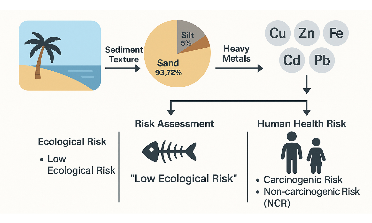
Rapid industrial growth and urban expansion have exacerbated the pollution of coastal beach sediments with heavy metals (HMs), particularly in developing countries such as Bangladesh, where the persistence and toxicity of these pollutants pose significant environmental and human health risks. Thus, this study investigated the contamination of HMs (Cu, Zn, Mn, Fe, Cd, Pb) to evaluate their associated risks at Kolatoli Beach, Cox’s Bazar, Bangladesh. Additionally, sediment texture analysis was performed to assess grain size distribution, which influences the mobility of these metals. The ecological risk (ER) was assessed through multiple indices, including the geo-accumulation index (Igeo), contamination factor (CF), pollution load index (PLI), ecological risk, and potential ecological risk index (PERI). Moreover, human health risk assessment (HHRA) was conducted for children and adults to determine non-carcinogenic and carcinogenic risks (CRs) through ingestion, inhalation, and dermal exposure. The sediment was predominantly sandy (93.72%), with lower clay (0%-2.51%) and silt (3.77%-6.28%) contents. The mean HM concentration in the sediment samples followed the descending order of Fe > Mn > Cu > Zn > Pb > Cd. The Igeo, CF, and PLI values indicated anthropogenic Cu and Pb accumulation in beach sediments, while Zn, Mn, and Fe remained at background levels. The PERI values ranged from 29.24 to 42.37, categorizing all samples under the ‘low ER’ classification (PERI < 150), though Pb and Cu had higher ER values. The overall hazard index (HI) values were below 1 for both age groups, indicating no significant non-carcinogenic risk (NCR). Total carcinogenic risk (TCR) values (5.99 × 10⁻⁶ for children, 3.99 × 10⁻⁶ for adults) remained within safe limits, though children posed higher CR. The statistical analyses revealed that HM contaminations were influenced by multiple factors. Overall, the study showed low to moderate HM contamination in the beach sediments, with tolerable ecological and human health risks.
Keywords
INTRODUCTION
Two-thirds of the world’s ice-free coastlines consist of sandy beaches, which serve as vital ecosystems and natural barriers against coastal erosion caused by waves, storms, tides, and rising sea levels. However, rapid coastal development over the past two centuries has significantly transformed these fragile environments. Activities such as sand mining, pollution, human recreation, and the disruption of natural sand transport have led to habitat degradation and ecosystem instability[1-3]. As the global population grows, increasing demand for coastal infrastructure and tourism further intensifies these pressures. Today, climate change adds a new dimension to coastal changes, exacerbating the vulnerability of sandy shorelines and accelerating environmental deterioration. Beaches are increasingly contaminated by heavy metals (HMs), as stated in numerous studies[4-6]. The rapid industrialization of coastal areas, driven by population growth and economic expansion, has led to the annual release and disposal of significant amounts of HM-laden waste into coastal environments[5]. These metals enter the coastal ecosystem, posing serious threats to marine life, including macrofauna on sandy beaches. As a result, human-induced HM pollution has become a growing concern. Major sources of contamination include sewage outlets, industrial production, mining activities, waste disposal, and shore nourishment practices[5].
Accumulation of HMs in coastal and marine environments is a rising global concern due to its ecological implications, persistence, and role in biogeochemical cycles[7]. Industrial waste, urban wastewater, and antifouling paints from ships contribute significantly to metal contamination in sediments, where metals accumulate through co-precipitation, adsorption, and hydrolysis[1]. While sediments act as a sink, environmental changes such as shifting wind patterns can remobilize these contaminants into the water column, increasing exposure risks for marine organisms and humans. Since benthic species are the foundation of the marine food web, the bioaccumulation of HMs can pose long-term ecological threats[8].
Regional studies highlighted the effects of industrialization and human activities on HM contamination in coastal sediments. In Chennai, India, the northern beaches exhibit two to three times higher amounts of Cr, Pb, and Zn compared to southern beaches due to the presence of industrial complexes, whereas the less-industrialized southern beaches, primarily used for tourism, show lower contamination levels[9]. Similarly, in northern Spain, Cd, Pb, and Zn pollution in beach sediments is linked to port activities and the proximity of metal and chemical industries that discharge industrial waste into coastal waters[10]. In Cuba, research on beach sediments across six resorts in Matanzas City confirms widespread HM pollution, emphasizing the global nature of coastal contamination[11].
Kolatoli Beach in Cox’s Bazar, Bangladesh, is a rapidly developing tourist destination that faces several environmental challenges[12]. These include pollution from recreational activities, improper waste disposal, and unregulated coastal development. Moreover, the beach’s proximity to commercial hubs and expanding infrastructure raises concerns about potential HM contamination, primarily from urban runoff, vehicular emissions, and tourism-driven activities[13,14]. Additionally, sediment texture plays a crucial role in influencing the mobility and retention of HMs in coastal environments[15,16]. Despite these concerns, there is no current baseline data on HM contamination in the sediments of this major recreational beach in southeastern Bangladesh. Establishing such a baseline is essential for evaluating the environmental health of the area and for identifying potential ecological and public health risks.
Thus, the aim of this study was (i) to quantify HM (Cu, Zn, Mn, Fe, Cd, Pb) concentrations in Kolatoli Beach sediments; (ii) to analyze sediment texture and its effect on HM mobility; (iii) to assess pollution levels and evaluate associated risks using indices such as geo-accumulation index (Igeo), contamination factor (CF), pollution load index (PLI), ecological risk (ER), and potential ecological risk index (PERI); (iv) to assess and evaluate the potential health risks to children and adults from HM exposure; and (v) to identify sources of HM contamination. The findings of this study will inform strategies for mitigating HM contamination and protecting both the coastal ecosystem and human health at Kolatoli Beach in Cox’s Bazar, Bangladesh.
MATERIALS AND METHODS
Study area
The study was conducted at Kolatoli Beach, situated in the coastal region of Cox’s Bazar, Bangladesh [Figure 1]. Kolatoli Beach is one of the most visited tourist destinations in the country, renowned for its golden sandy shoreline and serene environment. The area is a key part of the Cox’s Bazar tourist circuit, drawing visitors for its scenic views, beach activities, and natural beauty. The beach is exposed to both local and international tourists, which has influenced the surrounding environment and local economy.
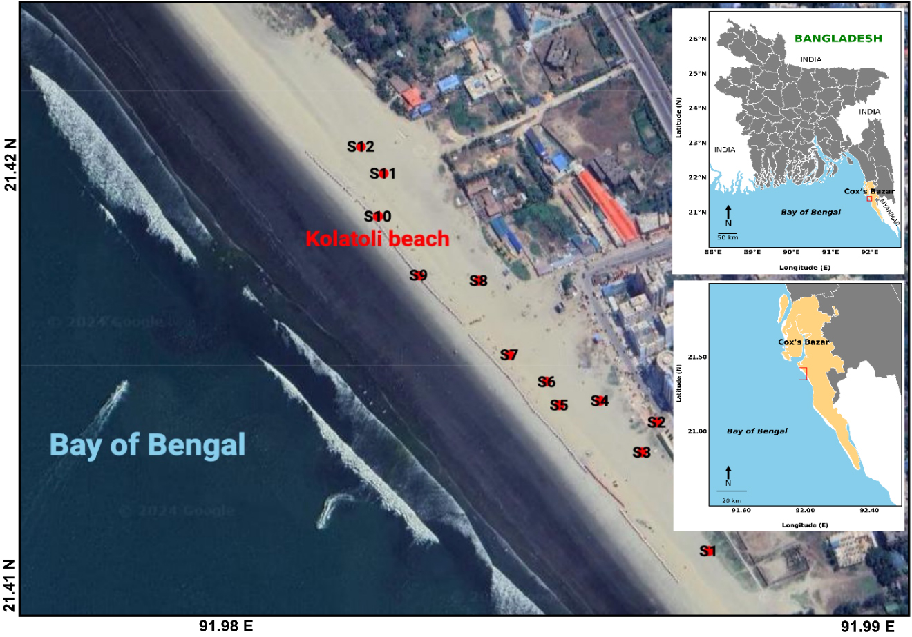
Figure 1. Map of the study area and sampling sites at Kolatoli Beach, Cox’s Bazar.
Geological information
Kolatoli Beach is located at coordinates 21°24’55’’N latitude and 91°58’57.1’’E longitude. The region is primarily composed of tertiary sediments, predominantly sandstones and shales. The geological landscape of the area is shaped by dynamic processes such as erosion, deposition, and sedimentation. The coastline is influenced by frequent cyclones and tsunamis, which continuously impact the coastal morphology, contributing to its ever-changing features. The combination of marine and terrestrial processes has created a unique coastal zone, with fine to medium sand and minimal organic content. The underlying alluvial deposits, mainly consisting of sand, silt, and clay, reflect the sedimentation patterns caused by river systems draining into the Bay of Bengal (BoB).
Sample collection and preparation
The field survey was conducted in December 2023. Surface sediment samples were collected from a total of 12 sampling sites [Figure 1]. At least three samples were taken randomly from each site. The exact locations were recorded using a handheld GPS device. The collected samples were placed in separate stainless-steel pans and air-dried for 48 h. After drying, 0.5 kg of each sample was carefully packed into clearly labeled polyethylene plastic bags. The bags were then sealed to prevent external contamination. The samples were then transported to the Soil Science Laboratory at University of Chittagong. In the Laboratory, samples were dried overnight in an oven at 45 °C. After drying, they were cooled in desiccators for 2 h. The cooled samples were then ground into fine powder using a mortar and pestle. Finally, they were stored in sealed plastic bottles at room temperature for further processing and analysis.
Sample digestion and HM determination
Sediment samples were digested using a block digestion system (Raypa, Terrassa, Barcelona, Spain). Analytical grade reagents (Sigma-Aldrich, Germany) and distilled water (DW) were used in this process. To prepare the digestion mixture, 2.5 mL of solution [0.42 g Se powder + 350 mL H2O2 + 420 mL concentrated sulfuric acid (H2SO4) (S.G. 1.84) + 14 g Li2SO4·H2O] was carefully added, then swirled and cooled. Afterward, 0.2 g of the sediment sample was taken in a digestion tube. After sample weighing, reagents were added to the sediment sample, and the digestion tubes were placed inside the heating block. The temperature was gradually increased and kept for 1.5 h after the clear appearance of the sediments at the bottom of the tubes. Following digestion, the solution was placed in a 50 mL polypropylene (PP) vial and filtered with Whatman filter paper (42). Finally, blank digestion was conducted using the reagents without a sediment sample. For HM contents, samples were analyzed using an atomic absorption spectrophotometer (Agilent Technologies 200 Series AA).
Certified reference materials from Sigma Aldrich were used to calculate equipment calibration curves for HM analysis [Supplementary Table 1]. DW was used throughout the analysis. Glassware used in the analyses was cleaned with 5% HNO3 and then repeatedly rinsed with deionized water and oven-dried.
Quality assurance and quality control
To ensure analytical accuracy and precision, comprehensive quality assurance and quality control (QA/QC) protocols were followed during sample preparation, digestion, and elemental analysis:
Method detection limits
The method detection limits (MDLs) for each HM were determined based on the standard deviation (SD) of multiple blank samples and are expressed in mg/kg sediment. The MDLs for the analyzed HMs have been explicitly reported in mg/kg sediment equivalent as follows: Cu (0.02), Zn (0.03), Mn (0.04), Fe (0.05), Cd (0.01), and Pb (0.02). These values have been added to the QA/QC section and are also listed in Supplementary Table 1.
Blank samples
Procedural blanks were analyzed at a ratio of 1 blank for every 5 sediment samples (i.e., n = 12 blanks total). These blanks contained only reagents without sediment. The detected concentrations of all target HMs in the blanks were consistently below detection limits (BDL), confirming minimal contamination during the analytical process.
Recovery assessment through matrix spikes
Recovery efficiency was assessed using matrix spike samples, where certified metal standards were spiked into known sediment matrices. A total of three matrix spike replicates were prepared for each metal at the following concentrations (soil equivalent basis): Cu-50 mg/kg, Zn-50 mg/kg, Mn-200 mg/kg, Fe-200 mg/kg, Pb-10 mg/kg, Cd-1 mg/kg. These concentrations were selected to reflect mid-range levels relative to environmental background values.
Recovery results and variability
The recovery rates for the spiked metals ranged from 92% to 105%. The reported recovery percentages represent mean values based on triplicate analysis, and their respective SDs were included to reflect reproducibility: Cu (95 ± 1.5%), Zn (97 ± 1.2%), Mn (98 ± 1.0%), Fe (96 ± 1.3%), Cd (94 ± 1.6%), and Pb (92 ± 1.8%).
The high recovery rates confirmed minimal matrix interference during digestion and analysis, supporting the robustness of the atomic absorption spectrophotometric method employed. These findings validate the reliability of the HM concentration data used in subsequent contamination and risk assessments.
Determination of physicochemical parameters
pH, electrical conductivity (EC), percentage of organic carbon (%OC), percentage of organic matter (%OM), and particle size distribution (along with textural classification) were analyzed. pH was determined with a glass electrode pH meter (EcoSense pH 1000A, USA) calibrated using pH standards of 4.0, 7.0, and 10.0. EC was determined using an EC meter (AD 330 EC/TDS Meter, Romania). For both pH and EC measurements, 5.0 g of sediment was placed into 50 ml PP tubes, and 25 mL of DW was added. The tubes were sealed and shaken on a horizontal shaker for 30 min, after which they were left to stand for an additional 30 min. The pH and EC values were then recorded using the respective meters.
Percent OC content in the sediment sample was measured using the wet-oxidation procedure outlined by Walkley and Black[17], modified by Allison[18]. To determine the %OC, 1.0 g of sediment was placed into a clean, dry 500 mL conical flask. Then, 10 mL of 1 N potassium dichromate (K2Cr2O7) was added with a pipette, followed by the addition of 10 mL of concentrated H2SO4. The mixture was thoroughly mixed, and the flask was placed on an asbestos sheet for 30 min, shaking occasionally, before allowing it to cool. After this, 150 mL of DW, 10 mL of H3PO4, 0.2 g of sodium fluoride, and 30 drops of (C6H5)2NH indicator were added. The contents of the flask, which turned a deep violet color, were then titrated with ferrous sulfate solution until the color changed to bottle green. Simultaneously, a blank was prepared using all the reagents without the sediment. The OM content in the sediment was calculated by multiplying the percentage of OC by the “Van Bemmelen factor” of 1.724, based on the hypothesis that soil OM consists of 58% carbon[18].
Precision of OC, OM, and EC measurements
The reproducibility of sediment physicochemical measurements was assessed by repeating each analysis in triplicate. The observed SDs were generally low. For example, when OC was reported as 0.05%, the typical precision was ± 0.01%. Similar precision was recorded for OM (± 0.017%) and EC (± 1.25 mS/m), indicating strong consistency of the measurements.
Sediment texture analysis
The hydrometer method was used to calculate the sediment’s particle size[19]. The textural categorization and particle size distribution were assessed by adding 100 mL of DW to 40 g of oven-dried sediment in a 600 mL beaker. Then, 5 mL of 30% H2O2 was introduced into the mixture, and the solution was heated on a hot plate for 15 min. After the solution had cooled, 100 mL of a 5% Calgon solution was added and stirred with a glass rod for 15 min. The beaker was then covered and left overnight. The following day, the contents were transferred into a 1L sedimentation cylinder, and the volume was adjusted to the mark using DW. Inside the cylinder, the solution was agitated with a paddle, and hydrometer measurements were taken cautiously at 40 s and after 2 h of sedimentation. Amendments were made to the hydrometer readings based on calibration at 20 °C. For the blank, 100 ml of Calgon solution was placed in a 1,000 mL cylinder that was filled with DW. The suspension was mixed carefully, and hydrometer readings, along with the temperature and blank readings, were recorded carefully.
The sediment samples were subsequently categorized based on their texture classes by plotting the amount of particle percentages (%sand, %silt, and %Clay) on a Marshall triangular diagram according to the United States Department of Agriculture guidelines. The particle percentages were calculated using Equations 1-4.
Where Rc at 40 secs is the hydrometer reading representing silt and clay in suspension, Rc at 2 h represents clay in suspension, and oven-dry wt is the weight of the sample dried at 105 °C.
Geo-accumulation index
The Igeo is a widely used technique for evaluating the extent of environmental pollution by comparing the present concentration of a substance (usually a HM) to its background or natural concentration[20-22]. The Igeo was calculated using the Equation 5[23].
Where Cb and Cs are the background and present concentrations of HMs in the sediments, respectively. These background values correspond to the concentrations of metals in the Earth's upper continental crust (UCC), which are 14.3, 52, 527, 30,890, 17, and 0.102 mg/kg for Cu, Zn, Mn, Fe, Pb, and Cd, respectively[24].
Müller introduced the Igeo with seven categories: (1) particularly pure (Igeo ≤ 0); (2) clean to moderately polluted (0 < Igeo ≤ 1); (3) moderately polluted (1 < Igeo ≤2); (4) moderately to strongly polluted (2 < Igeo ≤ 3); (5) strongly polluted (3 < Igeo ≤ 4); (6) strongly to tremendously polluted (4 < Igeo ≤ 5); and (7) tremendously contaminated (Igeo > 5)[23].
Potential ecological risk index
The PERI, proposed by Hakanson, was employed to assess the environmental risk posed by HMs in sediments. The calculations of PERI were carried out using a set of specific equations[25].
Firstly, the CF was calculated by evaluating the contamination level of a single metal using Equation 6.
Where Cb and Cs are the background and present concentrations of HMs in the sediments, respectively. The background concentrations of the metals in the Earth’s UCC are 14.3, 52, 527, 30,890, 17, and 0.102 mg/kg for Cu, Zn, Mn, Fe, Pb, and Cd, respectively[24]. Hakanson characterized the CF values into four classes: (1) low pollution (CF < 1); (2) moderate pollution (1 ≤ CF < 3); (3) substantial pollution (3 ≤ CF < 6); (4) very high pollution (6 ≤ CF)[25].
Secondly, the calculation of the ER, which assesses the possible environmental threat posed by a single HM, was derived from Equation 7.
Where Tr represents the toxic response factor of a single HM. The Tr values for Cu, Zn, Mn, Fe, Pb, and Cd are 5, 1, 1, 0, 5, and 30, respectively[25-29]. As per Hakanson, five categories for the ER are: (1) low risk (ER < 40); (2) moderate risk (40 ≤ ER < 80); (3) significant risk (80 ≤ ER < 160); (4) high risk (160 ≤ ER < 320); and (5) very high risk (ER ≥ 320)[25].
Finally, the PERI value was derived by summing up the ER values of all individual metals using Equation 8.
Hakanson classified the PERI values into four classes: (1) low risk (PERI < 150); (2) moderate risk (150 ≤ PERI < 300); (3) significant risk (300 ≤ PERI < 600); and (4) very high risk (PERI ≥ 600)[25].
Pollution load index
The PLI was proposed by Tomlinson et al.[30]. It was calculated using Equation 9.
Where “n” represents the number of metals analyzed, and CF refers to the contamination factor, as defined in Equation 6. The PLI provides an assessment of metal pollution levels and helps determine the required actions to address pollution. A PLI value of less than 1 signifies a pristine environment, a PLI of 1 indicates the occurrence of pollutants at baseline levels, and a PLI 1 reflects significant pollution[30].
Human health risk assessment
Human health risk assessment (HHRA) is a method used to evaluate the potential for adverse health effects in individuals exposed to environmental contaminants, either currently or in the future. This study performed an HHRA on sediments to determine the non-carcinogenic risk (NCR) and carcinogenic risk (CR) in humans via three main exposure routes: ingestion, inhalation, and dermal contact. The assessment followed the guidelines outlined by the US Environmental Protection Agency (EPA) and its Exposure Factors Handbook[31-33]. The chronic daily exposure (CDE) in mg/kg/day of HMs through ingestion
Where CDEing, CDEinh, and CDEdc are the daily amounts of exposure to metals (mg/kg/day) through ingestion, inhalation, and dermal contact, respectively. The definitions, factors influencing exposure, and the reference standards used for estimating intake levels and potential health risks of HMs in sediments are summarized in Table 1.
Definition, factors influencing exposure, and the reference standards for estimating HM intake and health risks in sediments
| Factors (unit) | Definitions | Values | References | |
| Children | Adults | |||
| Csediment (mg/kg) | HM concentration in sediment | - | - | - |
| IngR (mg/day) | Ingestion rate of sediment | 200 | 100 | [31] |
| InhR (m3/day) | Inhalation rate of sediment | 7.63 | 12.8 | [31] |
| EF (days/year) | Exposure frequency | 350 | 350 | [34] |
| ED (years) | Exposure duration | 6 | 24 | [31] |
| BW (kg) | Body weight of exposed individual | 15 | 55.9 | [34] |
| AT (days) | Average time | 365 × ED | 365 × ED | [33] |
| PEF (m3/kg) | Particle emission factor | 1.36 × 10⁹ | 1.36 × 10⁹ | [31] |
| SA (cm2) | Exposed skin surface area | 1,600 | 4,350 | [34] |
| AF (mg/cm day) | Skin adherence factor | 0.2 | 0.7 | [35] |
| ABF | Dermal absorption factor | 10-3 | 10-3 | [36] |
The potential health risks related to HM contamination from sediments were evaluated using hazard quotients (HQ) as per the United States Environmental Protection Agency (USEPA) health risk assessment procedures[37]. HQ quantifies NCRs. The overall NCRs are represented by the hazard index (HI), which was calculated by summing up the individual HQ[38].
Where reference dose (RfD) (mg/kg per day) is the highest acceptable daily dose of metal from a specific contamination pathway (both for children and adults). If the CDE is less than or equal to the RfD value (HQ ≤ 1), it is considered unlikely to cause negative health effects. Conversely, if the CDE surpasses the RfD value (HQ > 1), harmful health effects are likely to occur[5]. A HI value below 1.0 specifies no noteworthy NCRs, while an HI value 1.0 designates a probable occurrence of NCRs. The likelihood of NCRs rises as the HI value increases[39]. Table 2 provides the RfD values for the HMs analyzed in this study.
RfD values of HMs for each route of exposure
The CR quantifies the lifetime probability of developing cancer from exposure to carcinogenic HMs. It was calculated by multiplying the CDE and the corresponding slope factor (SF) for each metal using Equations 15-16.
For ingestion, the SF values are 0.0085 for Pb and 15 for Cd. For inhalation, the value is 6.3 for Cd and for dermal exposure, the value is 1.5 for Pb[42-44]. The optimal value of CR is measured as 10-4 by the USEPA, and the tolerable value is given as 10-6 to 10-4[38].
Statistical analyses
Hierarchical cluster analysis (HCA) was initially performed to classify the HMs based on their similarities, grouping them according to patterns of co-occurrence in the sediment samples. This analysis helps identify clusters of metals that exhibit similar contamination patterns and provides insights into the potential sources of the metals[45]. Following this, Pearson correlation analysis was used to examine the relationships between the metals. Positive correlations suggest that the metals likely originate from similar or common sources, while negative correlations indicate distinct sources[46]. Finally, principal component analysis (PCA) was performed to group sampling sites based on similarities in HM concentrations, revealing patterns in contamination profiles and aiding interpretation of spatial distribution and potential sources. The combination of these statistical techniques provides a robust framework for understanding the correlation between the HMs and their sources. All analyses were performed using the R programming environment (version 4.4.1).
RESULTS AND DISCUSSION
Sediment characteristics
Table 3 shows the sediment characteristics and particle size distribution in samples collected from Kolatoli Beach. The sediment texture across all samples was predominantly sandy. Sand consistently accounted for 93.72% of the composition. The clay and silt contents were comparatively lower than sand, ranging from 0% to 2.51% and 3.77% to 6.28%, respectively. This dominance of sand aligns with global observations in similar coastal regions, such as those reported by Ling et al., where sand proportions typically range from 49.4% to 99.7%[47].
Particle size distribution in the sediment samples collected from Kolatoli Beach
| Sample ID | pH | EC (mS/cm) | %OC | %OM | %Sand | %Silt | %Clay | Textural Class |
| K-1 | 8.75 | 19.99 | 0.109 | 0.188 | 93.72 | 3.77 | 2.51 | Sand |
| K-2 | 8.49 | 41.33 | 0.066 | 0.114 | 93.72 | 3.77 | 2.51 | Sand |
| K-3 | 8.43 | 69.63 | 0.175 | 0.301 | 93.72 | 3.77 | 2.51 | Sand |
| K-4 | 8.75 | 23.37 | 0.109 | 0.188 | 93.72 | 3.77 | 2.51 | Sand |
| K-5 | 8.81 | 18.25 | 0.175 | 0.302 | 93.72 | 3.77 | 2.51 | Sand |
| K-6 | 8.50 | 29.30 | 0.132 | 0.227 | 93.72 | 3.77 | 2.51 | Sand |
| K-7 | 8.72 | 24.67 | 0.131 | 0.227 | 93.72 | 3.77 | 2.51 | Sand |
| K-8 | 8.72 | 23.60 | 0.000 | 0.000 | 93.72 | 6.28 | 0.00 | Sand |
| K-9 | 8.61 | 58.17 | 0.110 | 0.190 | 93.72 | 3.77 | 2.51 | Sand |
| K-10 | 8.62 | 64.17 | 0.044 | 0.076 | 93.72 | 3.77 | 2.51 | Sand |
| K-11 | 8.66 | 57.97 | 0.044 | 0.076 | 93.72 | 3.77 | 2.51 | Sand |
| K-12 | 8.35 | 71.90 | 0.044 | 0.076 | 93.72 | 3.77 | 2.51 | Sand |
The sediment pH values ranged from 8.35 to 8.81, indicating an alkaline environment. It may be influenced by the intrusion of saline seawater and the presence of carbonate minerals derived from marine biota. Such conditions contribute to the precipitation of carbonate-metal complexes, stabilizing HMs in sediments. McCauley et al. reported that sediment pH is also influenced by OM content and carbonate deposition[48]. Additionally, EC values varied widely from 18.25 to 71.90 mS/m, reflecting differences in salinity and ionic concentrations due to tidal dynamics and proximity to the ocean. The %OC and %OM contents in the sediments were generally low across all sampling sites. OC ranged from 0.000% to 0.175%, and OM from 0.000% to 0.302%. Sample K-8 exhibited the lowest values, with both %OC and %OM recorded as 0.000%, while sample K-5 showed the highest %OC (0.175%) and %OM (0.302%) contents. This is expected given the sandy texture, which has a limited capacity to retain OM compared to finer sediments like clay. According to USDA, sandy soils generally have low OM due to their high infiltration rates and poor buffering capacity[49].
The uniformity in sediment texture suggests a strong hydrodynamic influence, where high wave energy facilitates the deposition of sand while removing finer particles. Similar observations were made by Bramha et al. on the Kalpakkam coast, where medium to coarse sands dominate due to local topographic and wave energy conditions[50]. The physicochemical factors such as pH, OC, OM, and EC are crucial in determining the bioavailability, mobility, and retention of HMs. Changes in pH can influence the solubility and the biogeochemical cycling of metals. Luo et al. highlighted that pH and OM directly affect HM mobility, emphasizing the importance of these parameters in assessing sediment quality[51].
Assessing heavy metal contamination
Table 4 summarizes the concentrations of HMs (mg/kg) in sediment samples from Kolatoli Beach, focusing on Cu, Zn, Mn, Fe, Cd, and Pb. The mean values for these metals were 6.09, 4.57, 347, 1.01 × 10⁴, and 4.30 mg/kg, respectively. Cd concentrations were BDL across all samples. The variability in concentrations is highlighted by SDs. When compared to established benchmarks such as the UCC[52] and USEPA Sediment Quality Guidelines (SQG)[53], Cu and Pb concentrations frequently exceed the thresholds for moderately polluted sediments. Meanwhile, Fe and Mn remained below their respective background values, indicating no significant contamination. These findings suggest localized pollution risks, particularly for Cu and Pb.
Mean concentration (mg/kg) of HMs in the sediment samples collected from Kolatoli Beach
| Sample ID | Cu | Zn | Mn | Fe | Cd | Pb | |
| K-1 | 5.86 × 101 | 5.63 × 101 | 3.16 × 10² | 1.20 × 10⁴ | BDL | 4.31 × 101 | |
| K-2 | 5.80 × 101 | 5.62 × 101 | 2.99 × 10² | 1.14 × 10⁴ | BDL | 4.15 × 101 | |
| K-3 | 5.95 × 101 | 7.27 × 101 | 3.10 × 10² | 1.17 × 10⁴ | BDL | 2.90 × 101 | |
| K-4 | 5.38 × 101 | 6.59 × 101 | 3.38 × 10² | 1.22 × 10⁴ | BDL | 3.48 × 101 | |
| K-5 | 6.64 × 101 | 4.47 × 101 | 3.81 × 10² | 1.09 × 10⁴ | BDL | 5.97 × 101 | |
| K-6 | 5.27 × 101 | 3.74 × 101 | 3.55 × 10² | 9.47 × 10³ | BDL | 7.63 × 101 | |
| K-7 | 4.76 × 101 | 4.28 × 101 | 3.86 × 10² | 7.88 × 10³ | BDL | 4.89 × 101 | |
| K-8 | 6.84 × 101 | 3.62 × 101 | 3.72 × 10² | 7.63 × 10³ | BDL | 3.73 × 101 | |
| K-9 | 6.13 × 101 | 3.41 × 101 | 3.45 × 10² | 7.96 × 10³ | BDL | 5.06 × 101 | |
| K-10 | 6.03 × 101 | 3.31 × 101 | 3.67 × 10² | 1.01 × 10³ | BDL | 2.32 × 101 | |
| K-11 | 6.77 × 101 | 3.62 × 101 | 3.38 × 10² | 1.01 × 10⁴ | BDL | 3.07 × 101 | |
| K-12 | 7.62 × 101 | 3.25 × 101 | 3.55 × 10² | 1.01 × 10⁴ | BDL | 4.06 × 101 | |
| Mean | 6.09 × 101 | 4.57 × 101 | 3.47 × 10² | 1.01 × 10⁴ | BDL | 4.30 × 101 | |
| SD | 7.52 × 100 | 1.38 × 101 | 2.81 × 101 | 1.95 × 10³ | BDL | 1.45 × 101 | |
| Upper continental crust[52] | 2.80 × 101 | 6.70 × 101 | 7.75 × 10² | 3.92 × 10⁴ | 9.00 × 10⁻³ | 1.70 × 101 | |
| SQG by | Not Polluted | < 2.50 × 101 | < 9.00 × 101 | < 3.00 × 10² | NA | - | <4.00 × 101 |
| USEPA[53] | Moderately Polluted | 2.50 × 101- 5.00 × 101 | 9.00 × 101- 2.00 × 101 | 3.00 × 10² | NA | < 6.00 × 100 | 4.00 × 101- 6.00 × 101 |
| Heavily Polluted | > 5.00 × 101 | > 2.00 × 101 | > 5.00 × 10² | NA | > 6.00 × 100 | > 6.00 × 101 | |
A comparative study of HM concentrations in Kolatoli Beach with other national and international studies is shown in Table 5. Kolatoli Beach showed higher levels of Cu, Zn, Mn, and Fe concentrations than many other regions, such as the Red Sea coast and Msasani Bay, but lower than the Ship Breaking areas. However, Pb concentrations were low to moderate compared to other locations. Kolatoli’s Cd concentration is BDL, contrasting with other regions, indicating lower contamination of Cd.
Comparison of mean HM concentrations (mg/kg) in the sediment samples from Kolatoli Beach with global studies
| Geographical area | Cu | Zn | Mn | Fe | Cd | Pb | Country | References |
| Kolatoli Beach | 60.9 | 45.7 | 347 | 10,100 | BDL | 43 | Bangladesh | Present study |
| Msasani Bay-Dar es Salaam harbour area | 13.5 | 58.4 | 133 | 7,250 | 3.6 | 35.4 | Tanzania | [54] |
| Red Sea coast | 14.6 | 40.5 | 193 | 15,700 | 3.97 | 19.5 | Egypt | [55] |
| Red Sea coast | 9.18 | 18 | 36.5 | - | 80 | 77.3 | Saudi Arabia | [56] |
| Red Sea coast (Shalateen) | 4.17 | 25.2 | - | - | 39 | 3.76 | Egypt | [28] |
| Eastern St. Martin’s Island | 3.76 | 27.2 | 270 | 144 | - | 5.88 | Bangladesh | [5] |
| Ship breaking area | 45.9 | 76.6 | 586 | - | - | 61.9 | Bangladesh | [57] |
| Ship breaking area | 255 | 1,230 | 1,080 | 93,000 | 49 | 68.3 | Bangladesh | [58] |
| Nijhum Dweep (Island) | 37 | 20.7 | 95.2 | 4,710 | 29 | 5.63 | Bangladesh | [22] |
| Sonadia Island | 18.1 | 38.8 | 390 | 15,100 | - | 9.03 | Bangladesh | [59] |
Assessment of contamination level
Geo-accumulation index
The Igeo values for the HMs at Kolatoli Beach are presented in Figure 2. According to Müller, the Igeo values for Cu (1.15-1.83) and Pb (-0.14-1.58) fall within the “moderately contaminated” (1 < Igeo ≤ 2) and “uncontaminated to moderately contaminated” (0 < Igeo ≤ 1) categories, respectively[23]. This suggests anthropogenic influences, potentially from tourism, fishing activities, or nearby industrial discharges, which are common sources of these metals in coastal environments[60]. In contrast, the consistently negative Igeo values for Zn (-1.26 to -0.10), Mn (-1.40 to -1.03), and Fe (-2.70 to -1.92) are within the “particularly uncontaminated” (Igeo ≤ 0) category, indicating that these metals are likely to derive from natural sources, such as weathering of bedrock and mineral deposits, rather than human activities[61,62]. These findings align with studies from other coastal regions, where Cu and Pb were often elevated due to anthropogenic activities, while Zn, Mn, and Fe remained at background levels[63]. Overall, the findings emphasized the necessity for monitoring and managing Cu and Pb to mitigate further contamination from these metals at Kolatoli Beach.
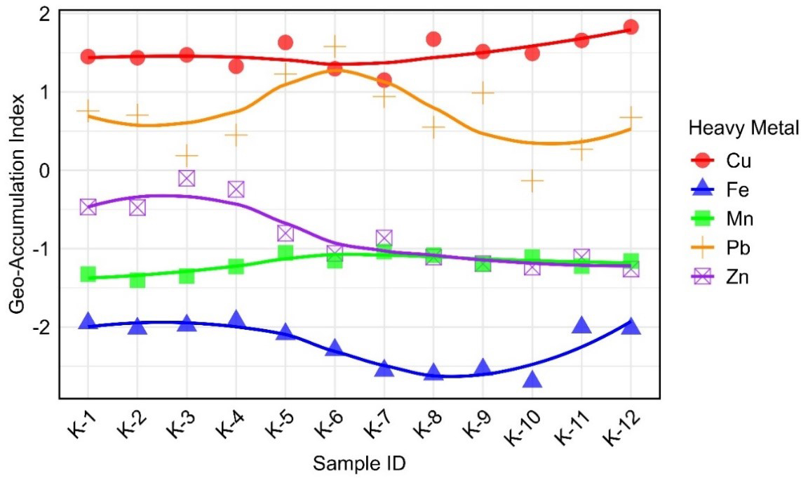
Figure 2. Igeo values of selected HMs across the sampling sites. Igeo: Geo-accumulation index; HM: heavy metal.
Contamination factor and pollution load index
The CF for the metals across the sampling sites is presented in Figure 3. According to Hakanson’s classification, Cu exhibited the highest contamination levels, with CF values ranging from 3.33 at site K-7 to 5.33 at site K-12, corresponding to the “moderate to high” and “high to very high” contamination categories, respectively[25]. Pb followed with CF values between 1.37 at K-10 and 4.49 at K-6, indicating “low to moderate” to “high” contamination. Zn showed lower contamination, with CF values ranging from 0.63 at K-12 to 1.40 at K-3, mostly categorized as “low” to “low to moderate” contamination. Mn demonstrated minimal contamination, with CF values ranging from 0.57 at K-2 to 0.73 at K-7, all within the “low” category. Fe exhibited the lowest CF values, ranging from 0.23 at K-10 to 0.40 at K-4, consistently indicating “low contamination”. Overall, Cu and Pb were the most contaminated metals, while Zn, Mn, and Fe showed relatively low contamination levels.
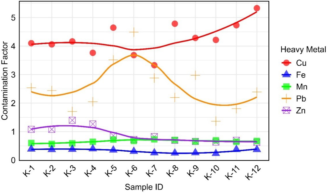
Figure 3. CF values of HMs across the sampling sites.CF: Contamination factor; HM: heavy metal.
The PLI is a quantitative tool for evaluating the extent of metal contamination in the environment, providing valuable insights into site quality and potential remediation requirements[30,57,64-66]. While the CF evaluates the pollution level of individual metals, the PLI reflects the combined impact of all analyzed metals at a site, providing a more comprehensive measure of overall contamination. In the present study, the PLI concentrations fluctuated between 0.90 and 1.29 across the sampling sites [Figure 4]. All values consistently exceeded the critical threshold of 1, except K-10 (0.90). Although the PLI value of K-10 is slightly below the threshold of 1, it remains close to this value, indicating a low but considerable level of contamination. These findings suggested a notable level of contamination across most sites, indicating the need for monitoring and possible remediation[67].
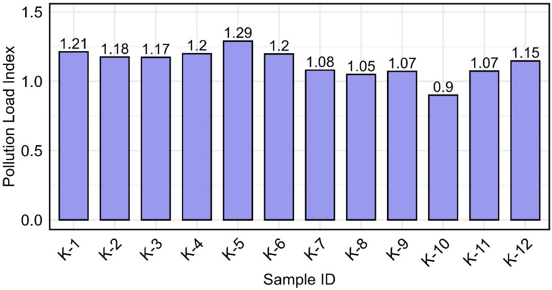
Figure 4. PLI values across the sampling sites. PLI :Pollution load index.
Risk assessment from metal contamination
Ecological risk and potential ecological risk index
The ER was calculated by multiplying the CF of each metal by its corresponding toxic response factor. The average ER values for all metals in a sample then resulted in the overall PERI[25]. Figure 5 shows the ER assessment of HMs in 12 sampling sites (K-1 to K-12), where the ER values of Cu, Zn, Mn, Fe, and Pb contributed to the PERI. According to Hakanson’s classification, all individual ER values for Zn, Mn, and Fe were relatively low[25]. However, Pb and Cu were the dominant contributors to PERI. The PERI values for all sampling sites ranged from 29.24 (K-10) to 42.37 (K-5), categorizing all samples under the ‘low ER’ classification (PERI < 150) [Figure 6]. This suggested that, based on the evaluated metals, the overall environmental risk in the study area remained minimal. However, Pb and Cu exhibited higher ER values than other metals, warranting further monitoring to assess potential ER. Implementing proactive measures, such as regulating industrial discharges and improving waste management, is essential to prevent long-term environmental degradation and protect the environmental integrity of the area[68-69].
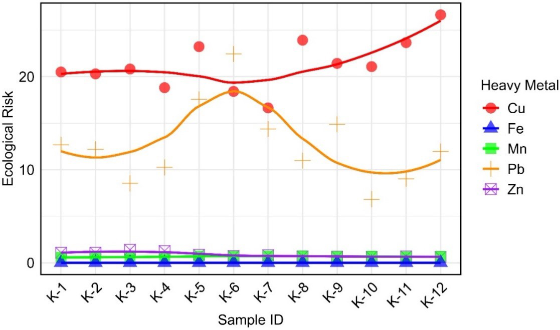
Figure 5. ER values of HMs across the sampling sites. ER: Ecological risk; HM: heavy metal.
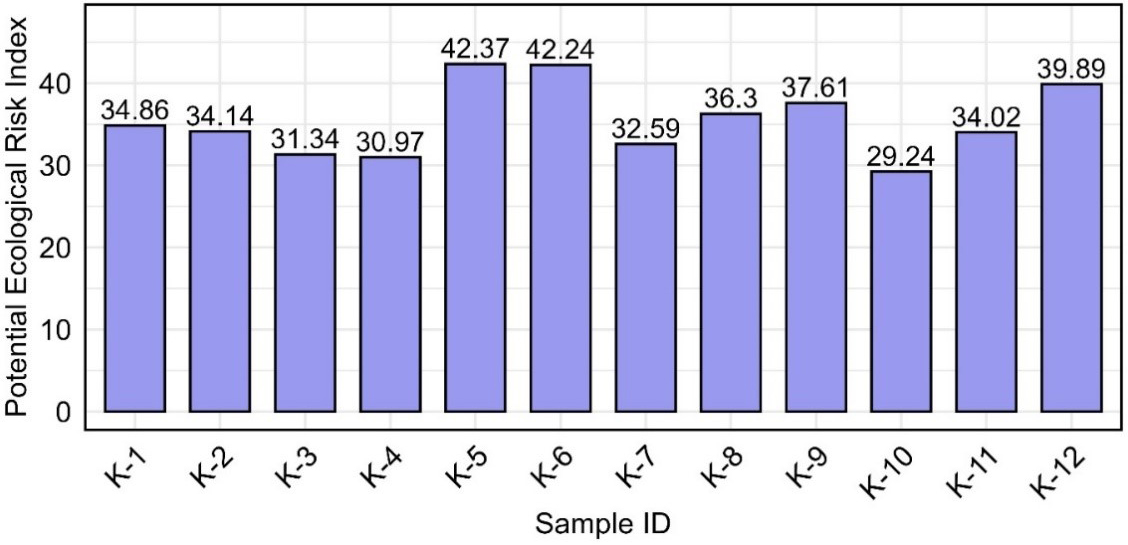
Figure 6. PERI values across the sampling sites. PERI: Potential ecological risk index.
Human health risk assessment
Chronic daily exposure
The CDE of metals was measured for both children and adults [Table 6]. The findings revealed that ingestion was the key contamination route, followed by dermal contact and inhalation. Children exhibited consistently higher CDE values than adults across all pathways, making them more vulnerable to metal exposure. Among the analyzed metals, Fe showed the highest CDE values in all exposure pathways, likely due to its higher concentration in the environment. Mn and Cu also contributed significantly to overall exposure. In contrast, Zn and Pb had the lowest CDE values.
Human health risk assessment for the HMs
| Metals | CDE | HQ | HI | CR | TCR | ||||||
| Ingestion | Inhalation | Dermal | Ingestion | Inhalation | Dermal | Ingestion | Inhalation | Dermal | |||
| Children | |||||||||||
| Cu | 7.78 × 10⁻⁴ | 2.18 × 10⁻⁸ | 1.25 × 10⁻⁶ | 1.95 × 10⁻² | 5.46 × 10⁻⁷ | 1.04 × 10⁻⁴ | 1.96 × 10⁻² | ||||
| Zn | 5.84 × 10⁻⁴ | 1.64 × 10⁻⁸ | 9.34 × 10⁻⁷ | 1.95 × 10⁻³ | 5.46 × 10⁻⁸ | 1.56 × 10⁻⁵ | 1.96 × 10⁻³ | ||||
| Mn | 4.44 × 10⁻³ | 1.24 × 10⁻⁷ | 7.10 × 10⁻⁶ | 9.64 × 10⁻² | 8.70 × 10⁻³ | 3.94 × 10⁻³ | 0.109 | ||||
| Fe | 0.129 | 3.63 × 10⁻⁶ | 2.07 × 10⁻⁴ | 1.54 × 10⁻² | 1.65 × 10⁻² | 2.95 × 10⁻³ | 3.48 × 10⁻² | ||||
| Pb | 5.50 × 10⁻⁴ | 1.54 × 10⁻⁸ | 8.79 × 10⁻⁷ | 0.157 | 4.38 × 10⁻⁶ | 1.67 × 10⁻³ | 0.159 | 4.67 × 10⁻⁶ | 1.32 × 10⁻⁶ | 5.99 × 10⁻⁶ | |
| Adults | |||||||||||
| Cu | 1.04 × 10⁻⁴ | 9.83 × 10⁻⁹ | 3.18 × 10⁻⁶ | 2.61 × 10⁻³ | 2.46 × 10⁻⁷ | 8.19 × 10⁻⁷ | 2.61 × 10⁻³ | ||||
| Zn | 7.84 × 10⁻⁵ | 7.37 × 10⁻⁹ | 2.39 × 10⁻⁶ | 2.61 × 10⁻⁴ | 2.46 × 10⁻⁸ | 1.23 × 10⁻⁷ | 2.61 × 10⁻⁴ | ||||
| Mn | 5.95 × 10⁻⁴ | 5.60 × 10⁻⁸ | 1.81 × 10⁻⁵ | 1.29 × 10⁻² | 3.92 × 10⁻³ | 3.11 × 10⁻⁵ | 1.69 × 10⁻² | ||||
| Fe | 1.73 × 10⁻² | 1.63 × 10⁻⁶ | 5.28 × 10⁻⁴ | 2.06 × 10⁻³ | 7.42 × 10⁻³ | 2.33 × 10⁻⁵ | 9.51 × 10⁻³ | ||||
| Pb | 7.37 × 10⁻⁵ | 6.94 × 10⁻⁹ | 2.25 × 10⁻⁶ | 2.11 × 10⁻² | 1.97 × 10⁻⁶ | 1.32 × 10⁻⁵ | 2.11 × 10⁻² | 6.27 × 10⁻⁷ | 3.37 × 10⁻⁶ | 3.99 × 10⁻⁶ |
Assessment of non-carcinogenic risk
The NCRs associated with HM exposure were evaluated using the HQ and HI values [Table 6]. The assessment revealed that the relative risk through ingestion was higher than through inhalation and dermal contact. For both children and adults, the highest HQ values were observed for Pb via ingestion. The mean HQ for Pb through ingestion was 1.57 × 10⁻¹ for children, significantly higher than the value for adults
Assessment of carcinogenic risk
The CR values for Pb in sediment samples were within permissible limits compared to the threshold (10-4) and the acceptable range (10-6 to 10-4) set by the USEPA. For children, the CR values from ingestion (4.67 × 10⁻⁶) and dermal contact (1.32 × 10⁻⁶) were within the acceptable range, indicating a relatively low CR. Similarly, the CR values for adults, both from ingestion (6.27 × 10⁻⁷) and dermal contact (3.37 × 10⁻⁶), were also within safe limits. The total carcinogenic risk (TCR) values, which combine ingestion, inhalation, and dermal pathways, provided a comprehensive measure of the overall risk[5,70]. The TCR values were 5.99 × 10⁻⁶ for children and 3.99 × 10⁻⁶ for adults. Both values were within the safe range. However, the TCR for children was higher than that for adults, demonstrating that children are more vulnerable to Pb-related CR. This finding is consistent with previous studies, which also reported a higher CR in children[38,76,77].
Source identification of metals in beach sediment
Hierarchical cluster analysis
Figure 7 illustrates the clustering of samples and HMs based on scaled concentrations [Figure 7A], highlighting two main clusters with distinct HM patterns. The accompanying histogram [Figure 7B] shows the distribution of scaled values. The first cluster (K-1, K-2, K-3, K-4) is characterized by low levels of Pb and Mn and moderate levels of Zn, Fe, and Cu. The second cluster (K-5, K-6, K-7, K-8, K-9, K-10, K-11, K-12) showed a more heterogeneous pattern, with K-5, K-6, K-7, and K-9 displaying significantly high levels of Pb but low levels of Zn, Cu, and Fe, indicating localized contamination[78,79]. On the variable axis, Zn and Fe were tightly clustered, suggesting a similar concentration trend across samples. Cu, Mn, and Pb formed another cluster, indicating potential co-occurrence of these metals[5]. The observed associations among elements suggest common geochemical or anthropogenic influences that affect their concentrations[45,80,81].
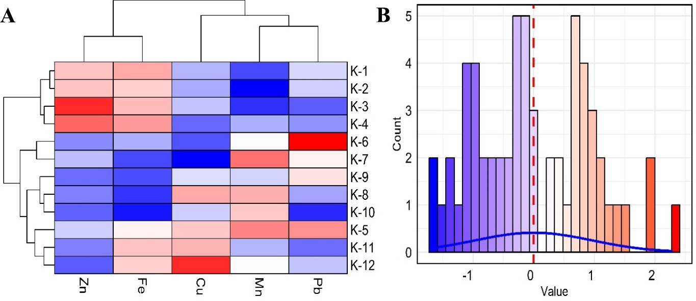
Figure 7. (A) Clustering heatmap of metal concentrations in Kolatoli beach sediments across 12 sites; (B) Color key and histogram.
Correlation analysis
The correlation matrix revealed distinct relationships among metals, soil properties, and their interactions [Figure 8]. Zn and Fe showed a strong positive correlation (r = 0.60), suggesting that they may originate from similar geochemical sources or processes. Moderately negative correlations were found between Mn and Zn (r = -0.50) and Fe and Mn (r = -0.45), suggesting competitive interactions and redox-driven mobility[82]. The other metal pairs exhibited very weak to weak correlations, indicating independent sources or localized contamination[5,38]. Among soil properties, pH and EC are negatively correlated (r = -0.701), reflecting how higher alkalinity reduces ionic conductivity. OC and OM are nearly identical (r = 0.9999), indicating their direct relationship. Silt and clay showed a perfect inverse correlation (r = -1.0), emphasizing their perfectly opposing roles in soil texture. This inverse relationship between silt and clay is significant because sediment texture directly influences metal mobility[83]. In terms of metal-soil interactions, Fe and Zn exhibited negative correlations with silt (Fe: r = -0.37; Zn: r = -0.21) and positive correlations with clay (Fe: r = 0.37; Zn: r = 0.21), indicating that finer-textured sediments with higher clay content tend to retain and accumulate these metals[84]. In contrast, Cu and Mn showed positive correlations with silt (Cu: r = 0.22; Mn: r = 0.24) and negative correlations with clay (Cu: r = -0.22; Mn: r = -0.24), indicating that coarser-textured sediments may enhance the mobility of these metals. Moreover, Pb and EC show a negative correlation (r = -0.455), implying reduced Pb solubility at higher ionic strengths. Zn and OC are positively correlated (r = 0.432), suggesting Zn accumulation in organic-rich soils. These correlations are crucial for identifying the sources and understanding the mobility of metals in the environment[46,85].
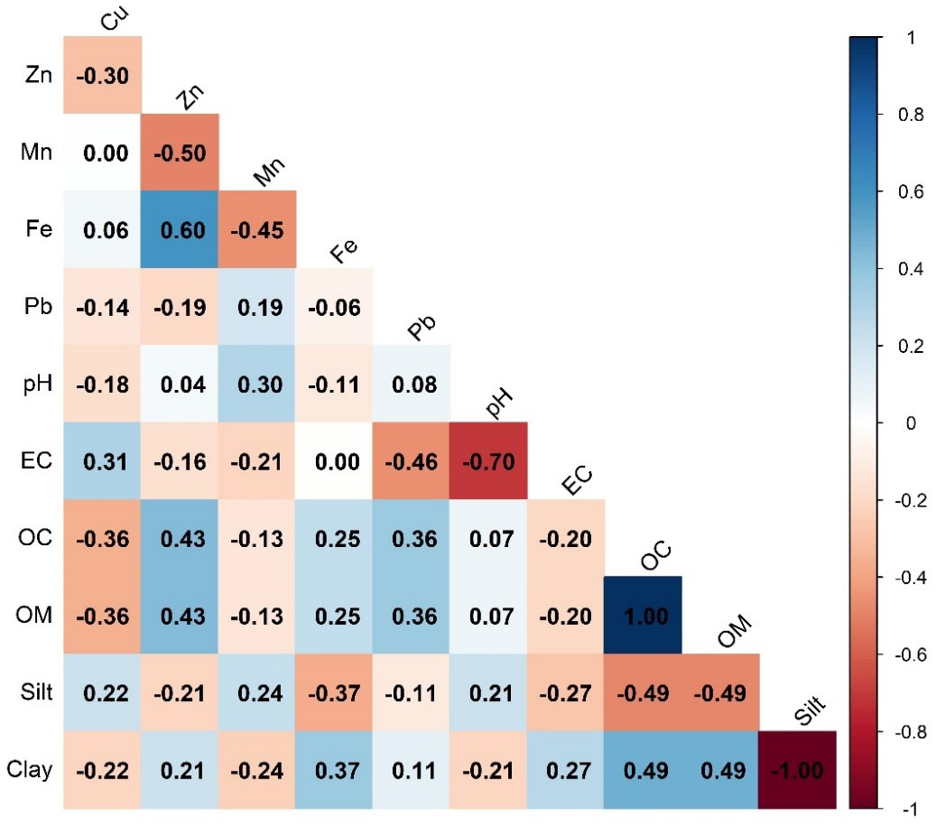
Figure 8. Pearson correlation coefficients among various HMs and sediment properties. HM: Heavy metal.
Principal component analysis
PCA is a commonly used multivariate statistical method that reduces the dimensionality of datasets with interrelated variables while retaining most of the variance[86]. To assess the suitability of a dataset for PCA, the Kaiser-Meyer-Olkin test is commonly used to evaluate sampling adequacy (MSA). The MSA value for the dataset in this study was 0.53, which falls within the marginal range of 0.5 to 0.7[87]. This suggests that the dataset has a moderate level of adequacy for PCA. The first three principal components explained a total of 83.38% of the variance in the dataset, with PC1 accounting for 42.08%, PC2 for 23.54%, and PC3 for 17.76% [Table 7]. Factor loadings [Table 8] showed that PC1 was mainly associated with Zn (-0.600), Fe (-0.548), and Mn (0.531), while PC2 was dominated by Cu (0.799), and PC3 by Pb (0.771), indicating variability in metal distribution patterns that may arise from both shared and distinct sources[45,88].
Percentage of variance and cumulative variances for the components
| PC | Variance (%) | Cumulative variance (%) |
| PC1 | 42.08 | 42.08 |
| PC2 | 23.54 | 65.61 |
| PC3 | 17.76 | 83.38 |
| PC4 | 11.09 | 94.47 |
| PC5 | 5.53 | 100 |
Factor loadings of the HMs on the first three PCs
| Parameters | PC1 | PC2 | PC3 |
| Cu | 0.106 | 0.799 | 0.456 |
| Zn | -0.600 | -0.212 | -0.106 |
| Mn | 0.531 | -0.121 | -0.086 |
| Fe | -0.548 | 0.057 | 0.423 |
| Pb | 0.214 | -0.546 | 0.771 |
The PCA biplots [Figure 9] depict the spatial distribution of metals across the sampling sites. In the PC1-PC2 biplot, sites K-1 to K-4 are linked with Zn and Fe, reflecting higher concentrations of these metals. Conversely, samples K-10 to K-12 show a strong association with Cu, suggesting localized Cu enrichment. Mn presents a mixed pattern, positive on PC1 and negative on PC2, mainly influencing sites K-5 and K-8. In the PC2-PC3 biplot, Cu and Fe show strong associations with sites K-2, K-5, K-9, K-11, and K-12, whereas Zn and Mn are associated with sites K-1 to K-4. Pb is predominantly linked to sites K-6 and K-7. These spatial patterns highlight variations in metal distribution across the study area. However, the lack of distinct clustering suggests that metal concentrations are more likely shaped by background variability than specific point sources. Nonetheless, anthropogenic activities remain a concern. The Karnafully River receives industrial discharges from tanneries, chemical plants, textile factories, and ship-breaking yards in Chittagong, which eventually flow into the BoB[89,90]. Additionally, atmospheric deposition from vehicles and tourist-related waste may further contribute to metal contamination.
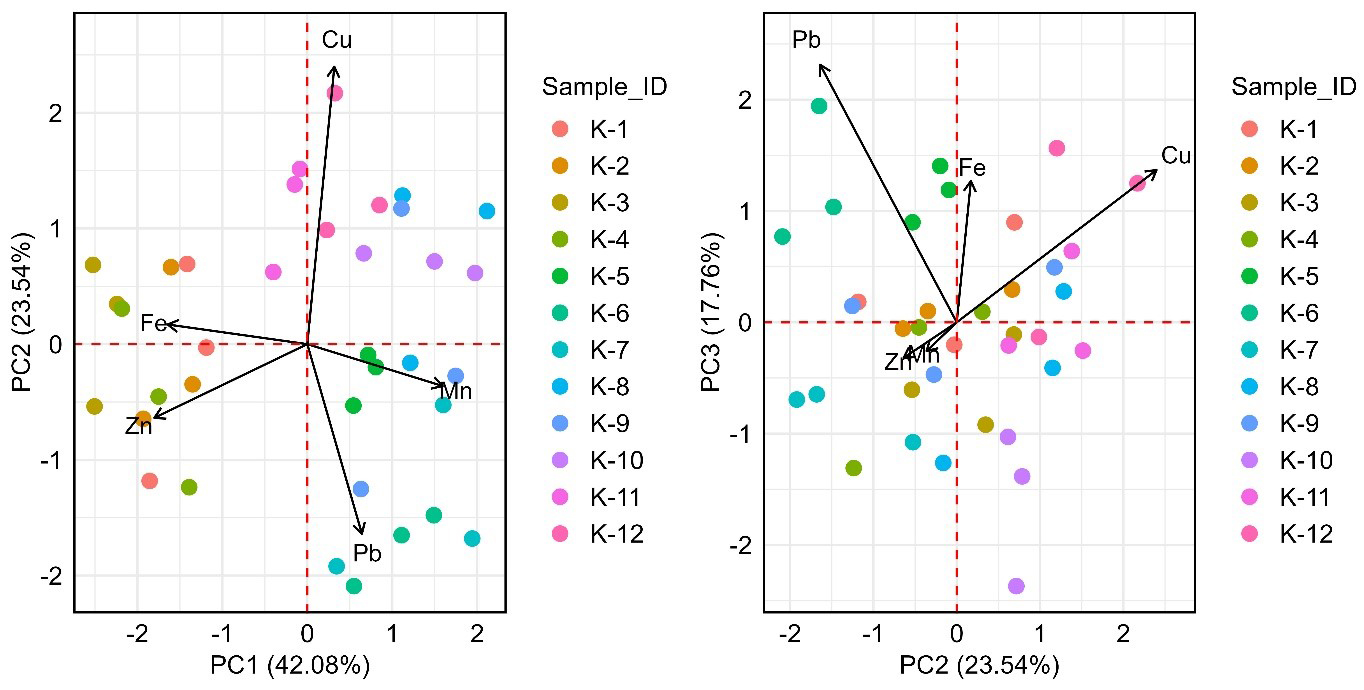
Figure 9. PCA biplots showing the spatial variations of metal composition among the 12 sites. PCA: Principal component analysis.
RECOMMENDATIONS FOR FUTURE WORK
In this study, samples were collected exclusively in December 2023 during the dry season, a period not influenced by significant runoff or dilution, thereby providing reliable baseline results. To further strengthen coastal monitoring and management efforts, future studies should incorporate seasonal sampling to capture temporal variations in HM concentrations influenced by monsoonal runoff and tourist activity. Source apportionment using advanced techniques such as isotopic tracing or metal speciation is recommended to identify and quantify specific anthropogenic inputs, including urban discharge, antifouling agents, and industrial effluents. Additionally, assessing the bioavailability of metals through sediment-porewater-biota partitioning would refine ER predictions by moving beyond total concentration metrics. Community awareness programs, particularly targeting children and other vulnerable groups, should also be developed to reduce direct exposure risks and enhance public engagement in environmental protection. These directions will deepen the understanding of contamination dynamics and support more effective policy responses for sustainable beach management.
CONCLUSIONS
The sediment analysis revealed that the beach was predominantly sandy, with low contents of clay and silt. The study indicated low levels of HM contamination, with Fe and Mn being the most abundant metals present in the sediments. Compared to other regional and global studies, contamination levels in this area were relatively lower. The Igeo, CF, and PLI values indicated anthropogenic Cu and Pb enrichment in beach sediments, while Zn, Mn, and Fe remained at background levels. The PERI values indicated higher ERs for Pb and Cu. This highlighted the critical role of Cu and Pb in influencing the overall sediment quality of Kolatoli Beach. These elevated levels of Cu and Pb may indicate localized anthropogenic pollution sources. The CDEs indicated that exposure primarily occurred through ingestion and exposure was consistently higher for children than for adults. Although the cumulative HI values reflected combined risks from all exposure pathways, they remained below 1 for both age groups, indicating no significant NCR in the region. The TCR values for both children and adults were within the safe range. However, the TCR for children was higher than that for adults, indicating greater vulnerability to CR in children. The hierarchical cluster, Pearson correlation, and PCA analyses revealed strong associations between Zn-Fe, indicating a shared geochemical origin and similar distribution patterns across samples. The inverse relationship between Mn-Zn and Fe-Mn observed in both correlation and PCA suggested competitive interactions affecting their mobility. Additionally, the cluster analysis identified localized Pb contamination, which aligns with PCA results showing a strong Pb loading in PC3. Cu’s dominance in PC2 and PC3 further highlights its distinct contamination source in the study area. The findings emphasize the importance of targeted interventions, especially for Pb and Cu, to mitigate environmental and public health risks. Integrating these results into policy will help ensure effective protection for both the environment and the public in Kolatoli Beach.
DECLARATIONS
Authors’ contributions
Conceptualization: Hossain, N.
Supervision: Hossain, N.
Methodology: Hossain, N.; Bhuyan, M.S.; Ismail, M.
Resources: Hossain, N.
Writing - original draft: Hossain, N.; Bhuyan, M.S.; Ismail, M.
Project administration: Bhuyan, M.S.
Writing- review & editing: Bhuyan, M.S.; Azwad, S.A.; Asif, M.R.; Iqbal M.M.
Software: Ismail, M.
Formal analysis: Hossain, N.
Visualization: Ismail, M.; Bhuyan, M.S.
Availability of data and materials
Data are available from the corresponding author upon reasonable request.
Financial support and sponsorship
None.
Conflicts of interest
All authors declared that there are no conflicts of interest.
Ethical approval and consent to participate
Not applicable.
Consent for publication
Not applicable.
Copyright
© The Author(s) 2025.
Supplementary Materials
REFERENCES
1. Bhuyan, M. S.; Kunda, M.; Bakar, M. A.; et al. Heavy metal and mineral analysis of cultivated seaweeds from Cox’s Bazar Coast, Bay of Bengal, Bangladesh: a human health risk implication. Discov. Oceans. 2024, 1, 12.
2. Pandey, S.; Kumar, G.; Kumari, N.; Pandey, R. Assessment of causes and impacts of sand mining on river ecosystem. In: Madhav S, Singh VB, Kumar M, Singh S, editors. Hydrogeochemistry of Aquatic Ecosystems. Wiley; 2023. pp. 357-79.
3. Bat, L.; Öztekin, A.; Arici, E.; Şahin, F.; Bhuyan, M. S. Trace Element risk assessment for the consumption of Sarda sarda (Bloch, 1793) from the mid-South Black Sea coastline. Water. Air. Soil. Pollut. 2022, 233, 5918.
4. Bisht, A.; Martinez-alier, J. Coastal sand mining of heavy mineral sands: contestations, resistance, and ecological distribution conflicts at HMS extraction frontiers across the world. J. Ind. Ecol. 2023, 27, 238-53.
5. Bhuyan, M. S.; Haider, S. M. B.; Meraj, G.; et al. Assessment of heavy metal contamination in beach sediments of Eastern St. Martin’s Island, Bangladesh: implications for environmental and human health risks. Water 2023, 15, 2494.
6. Yang, T.; Cheng, H.; Wang, H.; et al. Comparative study of polycyclic aromatic hydrocarbons (PAHs) and heavy metals (HMs) in corals, surrounding sediments and surface water at the Dazhou Island, China. Chemosphere 2019, 218, 157-68.
7. Goddard-Dwyer, M. Marine humic substances: distribution, cycling pathways, and biogeochemical function [dissertation]. University of Liverpool; 2024. Available from: chrome-extension://efaidnbmnnnibpcajpcglclefindmkaj/https://livrepository.liverpool.ac.uk/3187037/1/201508189_Jun2024.pdf (accessed on 2025-7-14).
8. Oros, A. Bioaccumulation and trophic transfer of heavy metals in marine fish: ecological and ecosystem-level impacts. J. Xenobiot. 2025, 15, 59.
9. Santhiya, G.; Lakshumanan, C.; Jonathan, M. P.; et al. Metal enrichment in beach sediments from Chennai Metropolis, SE coast of India. Mar. Pollut. Bull. 2011, 62, 2537-42.
10. Sanz-Prada, L.; García-Ordiales, E.; Roqueñí, N.; Grande, Gil. J. A.; Loredo, J. Geochemical distribution of selected heavy metals in the Asturian coastline sediments (North of Spain). Mar. Pollut. Bull. 2020, 156, 111263.
11. Rizo O, Buzón González F, Arado López JO, Denis Alpízar O. Heavy metal levels in dune sands from Matanzas urban resorts and Varadero beach (Cuba): assessment of contamination and ecological risks. Mar. Pollut. Bull. 2015, 101, 961-4.
12. Alam, J. Problems and prospects of the tourism industry in Bangladesh: a case of Cox’s Bazar tourist spots. Int. J. Sci. Bus. 2018, 2, 568-79.
13. Sahabuddin, M.; Tan, Q.; Hossain, I.; Alam, M. S.; Nekmahmud, M. Tourist environmentally responsible behavior and satisfaction; study on the world’s longest natural sea beach, Cox’s Bazar, Bangladesh. Sustainability 2021, 13, 9383.
14. Mohammad, B. T. An appraisal of the economic outlook for the tourism industry, specially Cox’s Bazar in Bangladesh. JECOM 2020, 1, 24-34.
15. Geng, N.; Xia, Y.; Li, D.; Bai, F.; Xu, C. Migration and transformation of heavy metal and its fate in intertidal sediments: a review. Processes 2024, 12, 311.
16. Liu, Q.; Yang, P.; Hu, Z.; Shu, Q.; Chen, Y. Identification of the sources and influencing factors of the spatial variation of heavy metals in surface sediments along the northern Jiangsu coast. Ecol. Indic. 2022, 137, 108716.
17. Walkley, A.; Black, I. A. An examination of the Degtjareff method for determining soil organic matter, and a proposed modification of the chromic acid titration method. Soil. Sci. 1934, 37, 29-38.
18. Allison, L. E.; Organic, carbon. In: Blac CA, editor. Methods of Soil Analysis: Part 2. Chemical and Microbiological Properties. Madison: American Society of Agronomy; 1965. pp. 1367-78.
19. Day, P. R. Particle Fractionation and particle-size analysis. In: Black CA, editor. Methods of Soil Analysis. Madison: American Society of Agronomy, Soil Science Society of America; 1965. pp. 545-67.
20. Saleem, M.; Pierce, D.; Wang, Y.; Sens, D. A.; Somji, S.; Garrett, S. H. Heavy metal(oid)s contamination and potential ecological risk assessment in agricultural soils. J. Xenobiot. 2024, 14, 634-50.
21. Panda, B. P.; Mohanta, Y. K.; Paul, R.; et al. Assessment of environmental and carcinogenic health hazards from heavy metal contamination in sediments of wetlands. Sci. Rep. 2023, 13, 16314.
22. Rahman, M. S.; Ahmed, Z.; Seefat, S. M.; et al. Assessment of heavy metal contamination in sediment at the newly established tannery industrial Estate in Bangladesh: A case study. Environ. Chem. Ecotox. 2022, 4, 1-12.
23. Müller, G. Index of geo-accumulation in sediments of the Rhine River. GeoJournal 1969, 2, 108-18. Available from: https://scispace.com/papers/index (accessed on 2025-7-14).
24. Wedepohl K. The composition of the continental crust. Geochimica. et. Cosmochimica. Acta. 1995, 59, 1217-32.
25. Hakanson, L. An ecological risk index for aquatic pollution control.a sedimentological approach. Water. Research. 1980, 14, 975-1001.
26. Saha, A.; Gupta, B. S.; Patidar, S.; MartínezVillegas, N. Evaluation of potential ecological risk index of toxic metals contamination in the soils. Chem. Proc. 2022, 10, 59.
27. Simeon, E. O.; Friday, K. Index models assessment of heavy metal pollution in soils within selected abattoirs in Port Harcourt, Rivers State, Nigeria. Singap. J. Sci. Res. 2016, 7, 9-15.
28. Soliman, N. F.; Nasr, S. M.; Okbah, M. A. Potential ecological risk of heavy metals in sediments from the Mediterranean coast, Egypt. J. Environ. Health. Sci. Eng. 2015, 13, 70.
29. Liu, J.; Li, Y.; Zhang, B.; Cao, J.; Cao, Z.; Domagalski, J. Ecological risk of heavy metals in sediments of the Luan River source water. Ecotoxicology 2009, 18, 748-58.
30. Tomlinson, D. L.; Wilson, J. G.; Harris, C. R.; Jeffrey, D. W. Problems in the assessment of heavy-metal levels in estuaries and the formation of a pollution index. Helgolander. Meeresunters. 1980, 33, 566-75.
31. USEPA. Baseline human health risk assessment: Vasquez Boulevard and I-70 Superfund Site, Denver, Colorado. Denver (CO): US Environmental Protection Agency, Region VIII; 2001:1-170. Available from: https://nepis.epa.gov/Exe/ZyPDF.cgi/P1006STM.PDF?Dockey=P1006STM.PDF (accessed on 2025-7-14).
32. USEPA. Exposure Factors Handbook (1997 Final Report). National Center for Environmental Assessment, Office of Research and Development; 1997: 1-201. Available from: https://cfpub.epa.gov/ncea/efp/recordisplay.cfm?deid=12464 (accessed on 2025-7-14).
33. USEPA. Risk Assessment Guidance for Superfund. Volume I Human Health Evaluation Manual (Part A). Washington, DC: U.S. Environmental Protection Agency;1989. Available from: https://www.epa.gov/sites/default/files/2015-09/documents/rags_a.pdf (accessed on 2025-7-14).
34. Yap, C. K.; Chew, W.; Al-Mutairi, K. A.; et al. Assessments of the ecological and health risks of potentially toxic metals in the topsoils of different land uses: a case study in Peninsular Malaysia. Biology. (Basel). 2021, 11, 2.
35. Barnes, D. G.; Dourson, M. Reference dose (RfD): description and use in health risk assessments. Regul. Toxicol. Pharmacol. 1988, 8, 471-86.
36. Chabukdhara, M.; Nema, A. K. Heavy metals assessment in urban soil around industrial clusters in Ghaziabad, India: probabilistic health risk approach. Ecotoxicol. Environ. Saf. 2013, 87, 57-64.
37. USEPA. Risk Assessment Guidance for Superfund (RAGS). Volume I: Human Health Evaluation Manual (HHEM). Part E: Supplemental Guidance for Dermal Risk Assessment. US EPA 2004, 1. Available from: https://www.epa.gov/sites/default/files/2015-09/documents/part_e_impl_2004_final_supp.pdf (accessed on 2025-7-14).
38. Şimşek, A.; Özkoç, H. B.; Bakan, G. Environmental, ecological and human health risk assessment of heavy metals in sediments at Samsun-Tekkeköy, North of Turkey. Environ. Sci. Pollut. Res. Int. 2022, 29, 2009-23.
39. Li, Z.; Ma, Z.; van, der. Kuijp. T. J.; Yuan, Z.; Huang, L. A review of soil heavy metal pollution from mines in China: pollution and health risk assessment. Sci. Total. Environ. 2014, 468-469, 843-53.
40. Zheng, X.; Zhao, W.; Yan, X.; Shu, T.; Xiong, Q.; Chen, F. Pollution characteristics and health risk assessment of airborne heavy metals collected from Beijing bus stations. Int. J. Environ. Res. Public. Health. 2015, 12, 9658-71.
41. Aguilera, A.; Cortés, J. L.; Delgado, C.; et al. Heavy Metal contamination (Cu, Pb, Zn, Fe, and Mn) in urban dust and its possible ecological and human health risk in Mexican cities. Front. Environ. Sci. 2022, 10, 854460.
42. Li, X.; Ding, D.; Xie, W.; et al. Risk assessment and source analysis of heavy metals in soil around an asbestos mine in an arid plateau region, China. Sci. Rep. 2024, 14, 7552.
43. Oni, A. A.; Babalola, S. O.; Adeleye, A. D.; et al. Non-carcinogenic and carcinogenic health risks associated with heavy metals and polycyclic aromatic hydrocarbons in well-water samples from an automobile junk market in Ibadan, SW-Nigeria. Heliyon 2022, 8, e10688.
44. Huang, S.; Li, Q.; Yang, Y.; et al. Risk assessment of heavy metals in soils of a lead-zinc mining area in Hunan Province (China). Kem. Ind. 2017, 66, 173-8.
45. Nur-e-alam, M.; Salam, M. A.; Dewanjee, S.; et al. Distribution, concentration, and ecological risk assessment of trace metals in surface sediment of a tropical Bangladeshi Urban river. Sustainability 2022, 14, 5033.
46. Yu, D.; Wang, J.; Wang, Y.; Du, X.; Li, G.; Li, B. Identifying the source of heavy metal pollution and apportionment in agricultural soils impacted by different smelters in china by the positive matrix factorization model and the Pb isotope ratio method. Sustainability 2021, 13, 6526.
47. Ling, S. Y.; Junaidi, A.; Mohd, Harun. A.; Baba, M. Geochemical assessment of heavy metal contamination in coastal sediment cores from Usukan Beach, Kota Belud, Sabah, Malaysia. J. Phys. :. Conf. Ser. 2022, 2314, 012008.
48. McCauley, A.; Jones, C.; Jacobsen, J. Soil pH and organic matter. Nutr. Manag. Modul. 2009, 8, 1-12. Available from:.
49. United States Department of Agriculture, Soil Conservation Service (USDA). Soil taxonomy: a basic system of soil classification for making and interpreting soil surveys. Soil Survey Staff U.S. Department Agriculture Handbook 436; U.S. Department Agriculture: 1975. Available from: https://www.nrcs.usda.gov/sites/default/files/2022-06/Soil%20Taxonomy.pdf (accessed on 2025-7-14).
50. Bramha, S. N.; Mohanty, A. K.; Satpathy, K. K.; et al. Heavy metal content in the beach sediment with respect to contamination levels and sediment quality guidelines: a study at Kalpakkam coast, southeast coast of India. Environ. Earth. Sci. 2014, 72, 4463-72.
51. Luo, J.; Sheng, B.; Shi, Q. A review on the migration and transformation of heavy metals influence by alkali/alkaline earth metals during combustion. J. Fuel. Chem. Technol. 2020, 48, 1318-26.
52. Rudnick, R.; Gao, S. Composition of the continental crust. Treatise on Geochemistry. Amsterdam: Elsevier; 2014.
53. USEPA. An overview of sediment quality in the United States (EPA 905/9-88-002). Office of Water Regulations and Standards, U.S. EPA Region 5; 1987. Available from: https://archive.epa.gov/water/archive/polwaste/web/pdf/overview.pdf (accessed on 2025-7-14).
54. Muzuka, A. Distribution of heavy metals in the coastal marine surficial sediments in the Msasani Bay-Dar es Salaam Harbour Area. West. Ind. Oc. J. Mar. Sci. 2009, 6.
55. Elgendy, A. R.; El, Daba. A. E. M. S.; El-Sawy, M. A.; Alprol, A. E.; Zaghloul, G. Y. A comparative study of the risk assessment and heavy metal contamination of coastal sediments in the Red sea, Egypt, between the cities of El-Quseir and Safaga. Geochem. Trans. 2024, 25, 3.
56. Halawani, R. F.; Wilson, M. E.; Hamilton, K. M.; et al. Spatial distribution of heavy metals in near-shore marine sediments of the Jeddah, Saudi Arabia region: enrichment and associated risk indices. JMSE 2022, 10, 614.
57. Hossain, M. S.; Ahmed, M. K.; Liyana, E.; et al. A case study on metal contamination in water and sediment near a coal thermal power plant on the eastern coast of Bangladesh. Environments 2021, 8, 108.
58. Hasan, A. B.; Reza, A. H. M. S.; Kabir, S.; Siddique, M. A. B.; Ahsan, M. A.; Akbor, M. A. Accumulation and distribution of heavy metals in soil and food crops around the ship breaking area in southern Bangladesh and associated health risk assessment. SN. Appl. Sci. 2020, 2, 1933.
59. Kabir, M. Z.; Deeba, F.; Majumder, R. K.; Khalil, M. I.; Islam, M. S. Heavy mineral distribution and geochemical studies of coastal sediments at Sonadia Island, Bangladesh. Nucl. Sci. Appl. 2018, 27, 2. Available from: https://baec.portal.gov.bd/sites/default/files/files/baec.portal.gov.bd/page/1f00cd0e_737d_4e2e_ab9f_08183800b7a2/Article%201.pdf (accessed on 2025-7-14).
60. Buzzi, N. S.; Menéndez, M. C.; Truchet, D. M.; Delgado, A. L.; Severini, M. D. F. An overview on metal pollution on touristic sandy beaches: Is the COVID-19 pandemic an opportunity to improve coastal management? Mar. Pollut. Bull. 2022, 174, 113275.
61. Zhou, Q.; Yang, N.; Li, Y.; et al. Total concentrations and sources of heavy metal pollution in global river and lake water bodies from 1972 to 2017. Global. Ecology. and. Conservation. 2020, 22, e00925.
62. Wang, S. L.; Xu, X. R.; Sun, Y. X.; Liu, J. L.; Li, H. B. Heavy metal pollution in coastal areas of South China: a review. Mar. Pollut. Bull. 2013, 76, 7-15.
63. Chakraborty, T. K.; Hossain, M. R.; Ghosh, G. C.; et al. Distribution, source identification and potential ecological risk of heavy metals in surface sediments of the Mongla port area, Bangladesh. Toxin. Reviews. 2022, 41, 834-45.
64. Hossain, M. B.; Sultana, J.; Pingki, F. H.; et al. Accumulation and contamination assessment of heavy metals in sediments of commercial aquaculture farms from a coastal area along the northern Bay of Bengal. Front. Environ. Sci. 2023, 11, 1148360.
65. Hassan, M.; Rahman, M. A. T.; Saha, B.; Kamal, A. K. I. Status of heavy metals in water and sediment of the Meghna River, Bangladesh. Am. J. Environ. Sci. 2015, 11, 427-39.
66. Islam, M. S.; Ahmed, M. K.; Habibullah-al-mamun, M.; Hoque, M. F. Preliminary assessment of heavy metal contamination in surface sediments from a river in Bangladesh. Environ. Earth. Sci. 2015, 73, 1837-48.
67. Nazir, A.; Hussain, S. M.; Riyaz, M.; Kere, Z.; Zargar, M. A.; L, K. K. D. Environmental risk assessment, spatial distribution, and abundance of heavy metals in surface sediments of Dal Lake-Kashmir, India. Environ. Adv. 2024, 17, 100562.
68. Siddiqua, A.; Hahladakis, J. N.; Al-Attiya, W. A. K. A. An overview of the environmental pollution and health effects associated with waste landfilling and open dumping. Environ. Sci. Pollut. Res. Int. 2022, 29, 58514-36.
69. Kibria, G.; Hossain, M. M.; Mallick, D.; Lau, T. C.; Wu, R. Monitoring of metal pollution in waterways across Bangladesh and ecological and public health implications of pollution. Chemosphere 2016, 165, 1-9.
70. Apori, S. O.; Giltrap, M.; Dunne, J.; Tian, F. Human health and ecological risk assessment of heavy metals in topsoil of different peatland use types. Heliyon 2024, 10, e33624.
71. Kabir,
72. Khan, A.; Khan, M. S.; Hadi, F.; Khan, Q.; Ali, K.; Saddiq, G. Risk assessment and soil heavy metal contamination near marble processing plants (MPPs) in district Malakand, Pakistan. Sci. Rep. 2024, 14, 21533.
73. Shetty, B. R.; Pai, B. J.; Salmataj, S. A.; Naik, N. Assessment of Carcinogenic and non-carcinogenic risk indices of heavy metal exposure in different age groups using Monte Carlo simulation approach. Sci. Rep. 2024, 14, 30319.
74. Kawichai, S.; Prapamontol, T.; Santijitpakdee, T.; Bootdee, S. Risk assessment of heavy metals in sediment samples from the Mae Chaem River, Chiang Mai, Thailand. Toxics 2023, 11, 780.
75. Li, B.; Deng, J.; Li, Z.; Chen, J.; Zhan, F.; He, Y.; et al. Contamination and health risk assessment of heavy metals in soil and ditch sediments in long-term mine wastes area. Toxics 2022, 10, 607.
76. Li, B.; Deng, J.; Li, Z.; et al. Contamination and health risk assessment of heavy metals in soil and ditch sediments in long-term mine wastes area. Toxics 2022, 10, 607.
77. Odochi, U. B.; Enimakpokpo, J.; Akaolisa, C. C. Z.; Agbasi, O.; Nwachukwu, H. Assessment of heavy metal contamination and health risks in road deposited sediments: a study in Owerri, Nigeria. EQ 2024, 35, 1-24.
78. Karmaker, K. D.; Khan, N.; Akhtar, U. S.; et al. First assessment of trace metals in the intertidal zone of the world's longest continuous beach, Cox’s Bazar, Bangladesh. Mar. Pollut. Bull. 2024, 207, 116928.
79. Khan, R.; Rouf, M. A.; Das, S.; et al. Spatial and multi-layered assessment of heavy metals in the sand of Cox’s-Bazar beach of Bangladesh. Reg. Stud. Mar. Sci. 2017, 16, 171-80.
80. Arora, S.; Saha, P.; Shende, A. D. Assessment of heavy metal pollution of surface water through multivariate analysis, HPI and GIS techniques. Water. Pract. Technol. 2025, 20, 148-67.
81. Jolaosho, T. L.; Mustapha, A. A.; Hundeyin, S. T. Hydrogeochemical evolution and heavy metal characterization of groundwater from southwestern, Nigeria: an integrated assessment using spatial, indexical, irrigation, chemometric, and health risk models. Heliyon 2024, 10, e38364.
82. Ilechukwu, I.; Osuji, L. C.; Okoli, C. P.; Onyema, M. O.; Ndukwe, G. I. Assessment of heavy metal pollution in soils and health risk consequences of human exposure within the vicinity of hot mix asphalt plants in Rivers State, Nigeria. Environ. Monit. Assess. 2021, 193, 461.
83. Ravisankar, R.; Tholkappian, M.; Chandrasekaran, A.; Eswaran, P.; El-taher, A. Effects of physicochemical properties on heavy metal, magnetic susceptibility and natural radionuclides with statistical approach in the Chennai coastal sediment of east coast of Tamilnadu, India. Appl. Water. Sci. 2019, 9, 1031.
84. Paramasivam, K.; Ramasamy, V.; Suresh, G. Impact of sediment characteristics on the heavy metal concentration and their ecological risk level of surface sediments of Vaigai river, Tamilnadu, India. Spectrochim. Acta. A. Mol. Biomol. Spectrosc. 2015, 137, 397-407.
85. Onwukeme, V. I.; Eze, V. C. Identification of heavy metals source within selected active dumpsites in southeastern Nigeria. Environ. Anal. Health. Toxicol. 2021, 36, e2021008-0.
86. Zhang, Q.; Zhang, X. Quantitative source apportionment and ecological risk assessment of heavy metals in soil of a grain base in Henan Province, China, using PCA, PMF modeling, and geostatistical techniques. Environ. Monit. Assess. 2021, 193, 655.
87. Huang, X.; Luo, D.; Zhao, D.; et al. Distribution, source and risk assessment of heavy metal(oid)s in water, sediments, and Corbicula Fluminea of Xijiang River, China. Int. J. Environ. Res. Public. Health. 2019, 16, 1823.
88. Chen, H.; Wu, D.; Wang, Q.; et al. The predominant sources of heavy metals in different types of fugitive dust determined by principal component analysis (PCA) and Positive matrix factorization (PMF) modeling in Southeast Hubei: a typical mining and metallurgy area in central China. Int. J. Environ. Res. Public. Health. 2022, 19, 13227.
89. Uddin, M. J.; Jeong, Y. K. Urban river pollution in Bangladesh during last 40 years: potential public health and ecological risk, present policy, and future prospects toward smart water management. Heliyon 2021, 7, e06107.
Cite This Article
How to Cite
Download Citation
Export Citation File:
Type of Import
Tips on Downloading Citation
Citation Manager File Format
Type of Import
Direct Import: When the Direct Import option is selected (the default state), a dialogue box will give you the option to Save or Open the downloaded citation data. Choosing Open will either launch your citation manager or give you a choice of applications with which to use the metadata. The Save option saves the file locally for later use.
Indirect Import: When the Indirect Import option is selected, the metadata is displayed and may be copied and pasted as needed.
About This Article
Special Issue
Copyright

Data & Comments
Data
0


Comments
Comments must be written in English. Spam, offensive content, impersonation, and private information will not be permitted. If any comment is reported and identified as inappropriate content by OAE staff, the comment will be removed without notice. If you have any queries or need any help, please contact us at [email protected].