

Algebraic and automated targeting for inter-region problems in terrestrial carbon management network
 0
0 
Graphical Abstract
Abstract
Climate change mitigation is a global challenge. Negative emission technologies (NETs) such as enhanced weathering (EW) are among the promising emerging techniques for CO2 capture. However, the optimal deployment of EW requires systematic planning tools. In this work, novel algebraic and automated targeting techniques are presented to locate the external outsourced capacity of the EW network. The results of the algebraic and automated targeting techniques may be plotted as the grand composite curve, which has a good visual interface that facilitates planning and discussion. Two examples involving single and multiple regions are solved to elucidate the newly extended methods. When EW sources are integrated across different regions, excess capacity of the EW regions is better utilised, which allows a greater extent of CO2 capture.
Keywords


 Download PDF
INTRODUCTION
Even though global consensus has been reached in the Paris Agreement to limit global temperature rise to 2.0 °C, while pursuing efforts to limit the rise to 1.5 °C, recent analysis showed that it is likely that the 1.5 °C rise may be exceeded by the year 2027[1]. It has also been reported that extreme climate incidents are occurring at a higher frequency in various parts of the world, which are closely related to climate change[2]. Hence, decarbonisation efforts have to be more aggressive in the coming years in order to abate the ever-challenging effects of climate change.
Apart from conventional CO2 mitigation measures such as energy efficiency improvement and adoption of renewables, the IPCC[3] has proposed the adoption of carbon dioxide removal through negative emission technologies (NETs). The latter include emerging techniques such as enhanced weathering (EW), direct air capture, biochar, bioenergy with carbon capture and storage, etc.[4,5]. NETs have several advantages over traditional decarbonisation measures; they allow the removal of historical CO2 emissions and offset positive emissions from sectors that are hard to decarbonise, e.g. transportation, agriculture, etc. Note, however, that large deployment of NETs is associated with various financial and technical challenges[4]. Hence, careful evaluation of NET deployment is necessary.
To allow large-scale deployment of NET in the near future, various systematic planning tools are necessary. Some of the process systems engineering and process integration tools developed in the past decades are believed to play a major role in large-scale deployment of CCS. One such promising tool is carbon emission pinch analysis (CEPA), which was first proposed for the optimal allocation of fossil and low-carbon energy resources in a carbon-constrained energy planning problem[6]. The main underlying principle of CEPA is rooted in process integration, i.e., performance setting prior to detailed design. In the past four decades, process integration tools have been well established and dedicated to various industrial resource allocation problems, such as energy conservation[7,8], material recovery[9,10], etc. In the seminal work of CEPA, a graphical tool of carbon emission pinch diagram was proposed to locate the minimum amount of low-emission renewables while subject to the maximum CO2 emission limit[6]. Various successful applications have been reported worldwide, such as those in America[11,12], Europe[13-17], Asia[18-20] and Oceania[21,22]. In each of these applications, CEPA methodologies were tailor-made to account for local conditions. For instance, in the case of Poland, CEPA was used to set realistic renewable targets in phasing out lignite and hard coal, as the earlier energy plan did not account for the growing number of electric vehicles in the country[17]. For the case of Bangladesh, Tarequzzaman et al.[20] outlined strategies to facilitate Bangladesh’s long-term energy plan, in order to achieve the intended nationally determined contributions emission limit.
In recent years, various extended works of CEPA have been reported. In general, these extensions were meant to address greenhouse gas and CO2 emissions in various settings. An important extension was reported by Tan et al.[23], where a graphical targeting tool was used for optimal deployment of NETs such as EW and bio-char networks. Besides, Mu et al.[24] integrated the concept of CEPA into a process graph in order to identify a raw material network of lower CO2 emissions. Another work on lowering CO2 emissions was reported by Zhang et al.[25], who applied CEPA principles for the tobacco industry. On the other hand, Chew et al.[26] made use of CEPA principles to optimise waste treatment system configurations while considering greenhouse gas reduction. In the work of Yang et al.[27], a modified CEPA pinch diagram was used to compare the different options of coastal ecosystems (such as mangrove forests, seagrass beds, and coral reefs).
In this work, the EW network synthesis problem is analysed. A novel algebraic targeting tool, along with its automated targeting variant, is proposed for the analysis. These newly extended tools allow rapid determination of rigorous network targets due to their numerical nature, hence overcoming cumbersome manual plotting and inaccuracy issues that are inherent in the graphical method[23]. The algebraic tool is highly welcomed as it may be implemented in spreadsheet software, which promotes its widespread usage among practitioners. In addition, the algebraic and automated targeting tools allow the generation of a new graphical tool, which facilitates analysis and discussion. Besides, this work is extended to single- and multiple-region problems. In the latter, sinks and sources of different regions may be allocated across the geographical border. These are the main novelties of this work, which complement the state-of-the-art of the current EW work.
The paper is structured as follows. In the following section, the problem statement for a terrestrial CMN is first given. Next, the basics of graphical targeting tools are explained. The newly proposed algebraic targeting method is next proposed, which is followed by its illustration in Example 1, which is a single-region problem. The algebraic targeting method is next extended into its automated targeting variant, which is then illustrated using Example 2, where an inter-region problem is solved. The paper is finally concluded and future research directions are suggested.
PROBLEM STATEMENT
The problem for synthesising a terrestrial CMN can be stated as follows[23]:
• Given CO2 sources i, which are mineral crushing plants with known annual production capacity (fSRi) and operating life (tSRi). The product of the two parameters is the CO2 output of each source (mSRi).
• Given n CO2 sinks, which are application sites with known annual (fSKj) and application rate limit (mSKj). Dividing the latter with former yields the minimum operating life of the sinks (tSKj).
The problem may be represented as a superstructure where CO2 sources are to be paired with CO2 sinks, as shown in Figure 1. The main assumption of this synthesis problem is that all sources and sinks available for pairing will commence their operation at the same time[23]. In other words, time constraints are not considered in the pairing problem.
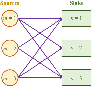
Figure 1. Superstructure representation of source-sink problem.
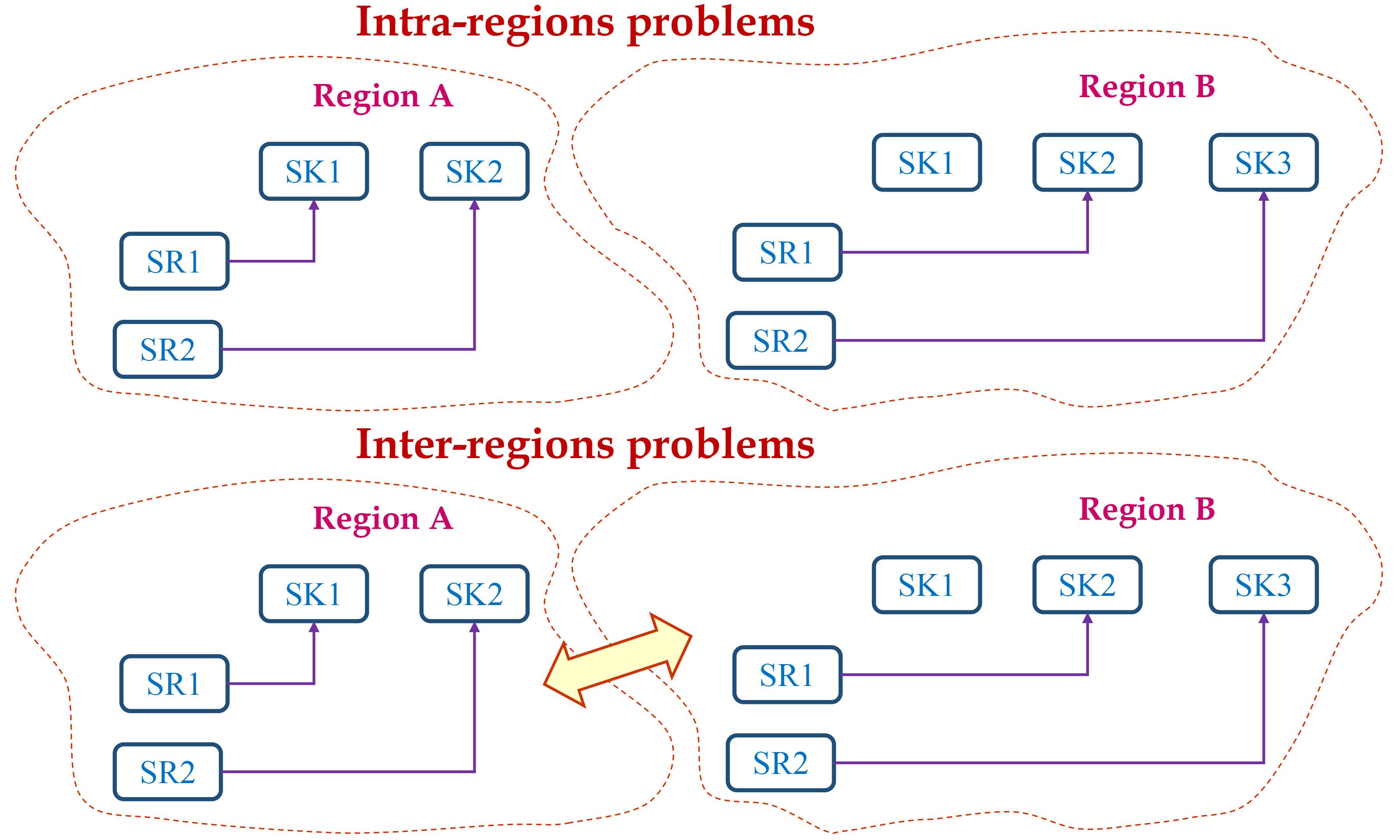
In this work, the main objective is to identify the capacity deficit and excess capacity targets of the terrestrial CMN by considering intra- and inter-region applications. For the former, all sinks and sources are located within a close distance, and hence the crushed mineral may be sent from plants (sources) to the application sites (sinks) within the same region. In another scenario involving inter-regional applications, various sources and sinks are found in separate regions (e.g., city, province) which are further from each other. For the case of inter-regions, CO2 sources may be sent to CO2 sinks within the same region, before they are sent to sinks in another region; doing so will maximise carbon sequestration, with reduced excess capacity deficit and excess CO2 load in the individual regions.
METHODS
In the work of Tan et al.[23], a graphical pinch diagram [Figure 2A] was proposed for the CO2 sink-source pairing problem. The tool identifies excess CO2 load from the CO2 sources (where outsourcing is needed), and their excess capacity once all CO2 loads are captured. The pinch diagram also identifies the pinch point, which is the bottleneck of the pairing problem, where capacity of the CO2 sinks run out. In this work, several other pinch analysis tools are extended for the terrestrial CMN problem.
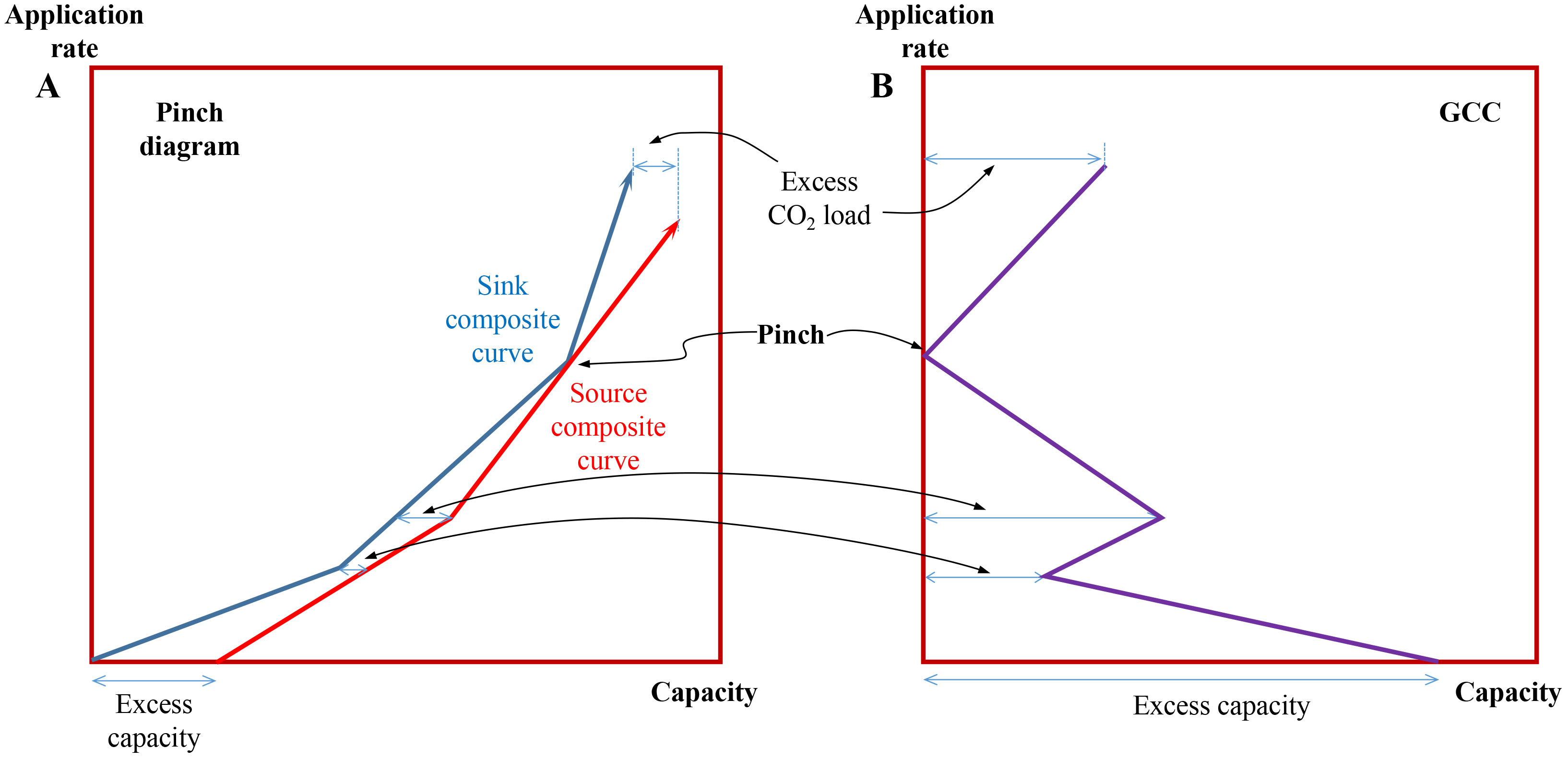
Figure 2. (A) The pinch diagram, and (B) the construction of the GCC from the pinch diagram. GCC: Grand composite curve.
Grand composite curve
The grand composite curve (GCC) was conventionally used in heat recovery problems[7]. Note that in the latter, the problem considered temperature and energy which are different from the terrestrial CMN problem in this work. In the latter, the GCC is plotted with application rate vs. the capacity. As shown in Figure 2B, the distance between the sink and source composite curves is first measured, which is then plotted on the x-axis (the y-axis remains identical to the pinch diagram) of the GCC. For a GCC, a segment that has a negative slope indicates that the capacity difference between the sources and sinks is reducing. On the other hand, a positive slope segment means that the capacity difference is increasing. Note that zero capacity difference indicates that a pinch is found (see Figure 2B). Openings at the top and bottom of the GCC indicate deficit and surplus (where excess 2 load is found) capacity, respectively, identical to those of the pinch diagram. One may also locate the “CO2 capture pocket” in the GCC, where CO2 sources are sent to the sinks [Figure 3]. Note, however, that the drawing exercise to construct the GCC (in Figure 2) is tedious, apart from not being able to determine the rigorous targets. Hence, more efficient methods are proposed in this work, which are based on algebraic and automated procedures. The former is first described in the following section.
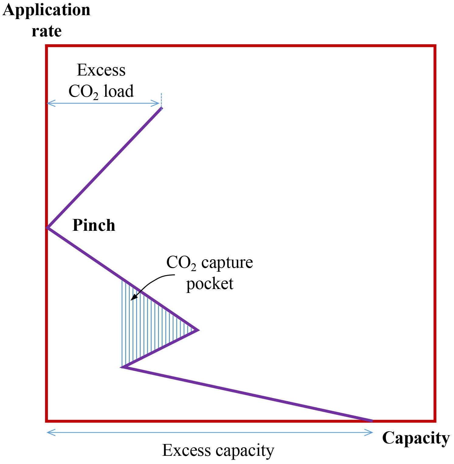
Figure 3. A generic GCC with its CO2 capture pocket. GCC: Grand composite curve.
ALGEBRAIC METHOD - CASCADE ANALYSIS
The algebraic tool has the following steps:
1. The sinks and sources are arranged in descending order of their operating life.
2. The application rates of the sinks (fSKj) and sources (fSRi) are added to form their cumulative values, i.e., Cum. fSKj and Cum. fSRi, respectively.
3. All cumulative application rates are then arranged in ascending order, with duplicates removed. These cumulative rates become the levels of the EW cascade and they are indicated as level k (Cum. fk); a generic form of these cumulative rates is shown in column 1 of Table 1.
Generic structure of the algebraic method
| Cum. fk | ∆fk | SKj | SRi | ∆mSK,k | ∆mSR,k | rk | Cum. rk | Revised Cum. rk |
| Cum. f1 | ↓ | ↓ | Cum. r1 = 0 | Cum. r1 = rEC | ||||
| ∆f1 | ↓ | ↓ | ∆mSK,1 | ∆mSR,1 | r 1 | |||
| Cum. f2 | ↓ | ↓ | Cum. r2 | Cum. r2 | ||||
| … … | … … | … … | … … | … … | … … | … … | … … | … … |
| Cum. fk | Cum. rk = rLD |
4. In column 2 of Table 1, the interval rates (∆fk) are calculated as the differences of the adjacent levels k, as follows
5. Within each interval, the sinks and sources are first located in columns 3 and 4, respectively.
6. Next, the interval capacities of the sinks (∆mSK,k) and interval load of the sources (∆mSR,k), are calculated using Equations 2 and 3, respectively. These values are documented in columns 5 and 6, respectively.
7. In column 7, the net capacity between the sinks and sources within each interval (rk) is calculated using
A positive value indicates that the CO2 sources are sufficient to meet the demand in the interval; a negative value means that the demand is not fulfilled.
8. The net capacity values are then accumulated downwards to form the capacity cascade in column 8, as follows
For a feasible capacity cascade, all net capacity values have to be positive, or at least zero - indicating that CO2 sink capacity is large enough to capture the CO2 load from the sources. If negative value(s) are observed, the capacity cascade is considered infeasible; Step 9 is to be followed.
9. The feasibility can be restored by identifying excess capacity (rEC) of the CO2 sink; the latter is identified with the largest deficit among the cascaded values in column 8.
10. The absolute value of the largest deficit is returned as the Cum. r1 value, located at the highest level in the EW cascade. The revised EW cascade will have all positive cascaded values, with zero value(s) indicating the pinch point of the sink-source matching problem, and may be viewed as the bottleneck of the CO2 capture capacity. The last entry of the revised EW cascade indicates the excess or uncaptured load (rLD) of the CO2 sources.
11. Lastly, the cumulative carbon dioxide removal (Cum. CDR) can be calculated by multiplying the summation of carbon sequestration factor (α) and the CO2 footprint per unit crushed rock allocated from source i to sink j (βij) with the total amount of rock supply from sources to sinks (R), as follows:
Note that the summation of α and β gives the net carbon dioxide balance per unit of rock. Generally, the α value is negative and is substantially larger than β (Tan and Aviso, 2019)[29]. In this work, the values of α and βij are taken as mean values reported in the literature. In actual implementation, their values may vary depending on factors such as particle size distribution, environmental conditions (pH, temperature, moisture), which affect the α value, as well as crushing, transportation, etc., that affect the β value. However, the methodology proposed in this work is based on process integration philosophy where the network performance targets are set in advance in priority to detailed analysis. This is in line with other process integration works such as heat recovery[7,8], water minimisation[8,9], property integration[9], etc.
The advantage of the EW cascade is that column 1 (Cum. fk) can be plotted against column 9 (Revised Cum. rk) to form the GCC [Figure 3]; the latter provides visualisation on the sink-source matching problem. Due to the algebraic nature of the procedure, the GCC construction is much simpler as compared to the plotting of GCC from the composite curve [Figure 2A].
Example 1
Example 1 is based on a literature case study[23]. For this example, basalt that is widely available and is commonly used in EW is chosen as the feedstock[28]. There are five sinks and three sources in this case study. It is assumed that the sinks and sources begin to operate at the same time but their economic service lifes may differ. For this case study, α is assumed to be -0.3 kt CO2/kt rock while all β values are assumed to be 0.05 kt CO2/kt rock[29]. The data for the sinks and sources are given in Table 2. As shown, all sinks and sources have been arranged in descending order of their operating life (step 1).
Data for Example 1 (Tan et al., 2021)[23]
| SKj | f SK j (kt/y) | t SK j (y) | m SK j (kt) | SRi | f SR i (kt/y) | t SR i (y) | m SR i (kt) | |
| 1 | 2.5 | 40 | 100 | 1 | 2.5 | 30 | 75 | |
| 2 | 0.6 | 25 | 15 | 2 | 1 | 25 | 25 | |
| 3 | 1.11 | 18 | 20 | 3 | 2 | 20 | 40 | |
| 4 | 1 | 15 | 15 | |||||
| 5 | 0.5 | 10 | 5 | |||||
| 155 | 140 |
In step 2, the application rates of the sinks (fSKj) and sources (fSRi) are added to form their cumulative values (Cum. fSKj for sinks and Cum. fSRi for sources; see Table 3). Following step 3, all cumulative rates of sinks and sources are arranged in ascending order, and form the levels of EW cascade in Table 4 (Cum. fk; see column 1).
Cumulative application rates for sinks and sources in Example 1
| f SK j (kt/y) | Cum. fSKj (kt/y) | f SR i (kt/y) | Cum. fSRi (kt/y) |
| 2.5 | 2.50 | 2.5 | 2.50 |
| 0.6 | 3.10 | 1 | 3.50 |
| 1.11 | 4.21 | 2 | 5.50 |
| 1 | 5.21 | ||
| 0.5 | 5.71 |
Cascade table for Example 1
| Cum. fk (kt/y) | ∆fk (kt/y) | SKj | SRi | ∆mSK,k (kt) | ∆mSR,k (kt) | rk (kt) | Cum. rk (kt) | Revised cum. rk (kt) |
| 0 | ↓ | ↓ | r 1 = 0 | 25 (rEC) | ||||
| 2.5 | SK1 | SR1 | 100 | 75 | -25 | |||
| 2.50 | ↓ | ↓ | -25 | 0 (pinch) | ||||
| 0.6 | SK2 | SR2 | 15 | 15 | 0 | |||
| 3.10 | ↓ | ↓ | -25 | 0 (pinch) | ||||
| 0.4 | SK3 | SR2 | 7.2 | 10 | 2.8 | |||
| 3.50 | ↓ | ↓ | -22.2 | 2.8 | ||||
| 0.71 | SK3 | SR3 | 12.8 | 14.2 | 1.4 | |||
| 4.21 | ↓ | ↓ | -20.8 | 4.2 | ||||
| 1.00 | SK4 | SR3 | 15.0 | 20.0 | 5.0 | |||
| 5.21 | ↓ | ↓ | -15.8 | 9.2 | ||||
| 0.29 | SK5 | SR3 | 2.9 | 5.8 | 2.9 | |||
| 5.50 | ↓ | ↓ | -12.9 | 12.1 | ||||
| 0.21 | SK5 | 2.1 | -2.1 | |||||
| 5.71 | 10 (rLD) |
In column 2 of Table 4, the differences between each adjacent cumulative rate level k (∆fk) are calculated using Equation 1 (step 4). In columns 3 and 4, the sinks and sources are located. As shown, some of them (e.g. SK1, SK2, SR1) only exist within one interval, while some others (e.g. SK3, SR2, SR3) cut across several intervals. Next, interval capacities for the sinks (∆mSK,f) and sources (∆mSR,f) are calculated in columns 5 and 6, respectively, following Equations 2 and 3 (steps 5 and 6).
In column 7, the net capacity between sinks and sources is calculated for each interval (rk; step 7). Negative values are observed in the first and last intervals (r1 = -25 kt; r7 = -2.1 kt), indicating a capacity deficit. On the other hand, positive values in other intervals (r2 – r6) indicate extra capacity in these intervals.
The net capacity values are then accumulated downwards following Equation (5), to form the capacity cascade. As shown in column 8, negative cumulative capacities are observed in all levels, indicating infeasibility for the capacity cascade. To restore feasibility, the absolute value of the largest r deficit value (25 kt) is identified (Equation 6) and returned as the highest level of column 9 in Table 4 (Equation 7); this corresponds to excess capacity of the CO2 sinks (rEC). In other words, SK1 may still sequester 25 kt of CO2 from other sources. In the last level of the EW cascade in column 9, 10 kt of excess CO2 load (rLD) is observed. This load can no longer be sent to the sinks due to their capacity limit; hence, new sinks will have to be explored (e.g., via inter-region integration; see Example 2). Based on Equation 9, the total amount of crushed basalt that can be supplied from the sources to the sinks is 130 kt (= 155 - 25 kt). Next, Equation 8 determines that the total CDR of the problem is calculated as -32.5 kt (= 130 × (-0.3 + 0.05) kt). If all β values are assumed to be 0 kt CO2/kt rock, the total CDR of the problem will be -39kt which is in agreement with those reported by Tan et al.[23].
An important insight of this EW problem is the pinch point(s) of the problem. Column 9 in Table 4 shows that two pinch points are found for this problem, i.e., at levels 2.5 and 3.1 kt/y. These pinch points indicate the bottlenecks of the EW problem. In regions with levels lower than 2.5 kt/y, the CO2 sinks have excess capacity (25 kt), but all CO2 loads from the sources have been sequestered. On the other hand, in regions with levels higher than 3.1 kt/y, all capacities of the CO2 sinks are utilised; however, there are still CO2 load from the sources, which requires the exploration of additional CO2 sinks.
With the algebraic targeting results in Table 4, one may plot the GCC with data in column 1 vs. column 9. As shown in Figure 4, the excess capacity of the CO2 sink is found at the bottom, i.e., 25 kt, while the opening at the top indicates excess CO2 load, i.e., 10 kt. Two pinch points are identified as well, i.e., 2.5 and 3.1 kt/y, identical to those reported by Tan et al.[23]. Besides, a CO2 capture pocket is identified at the top section of the GCC.
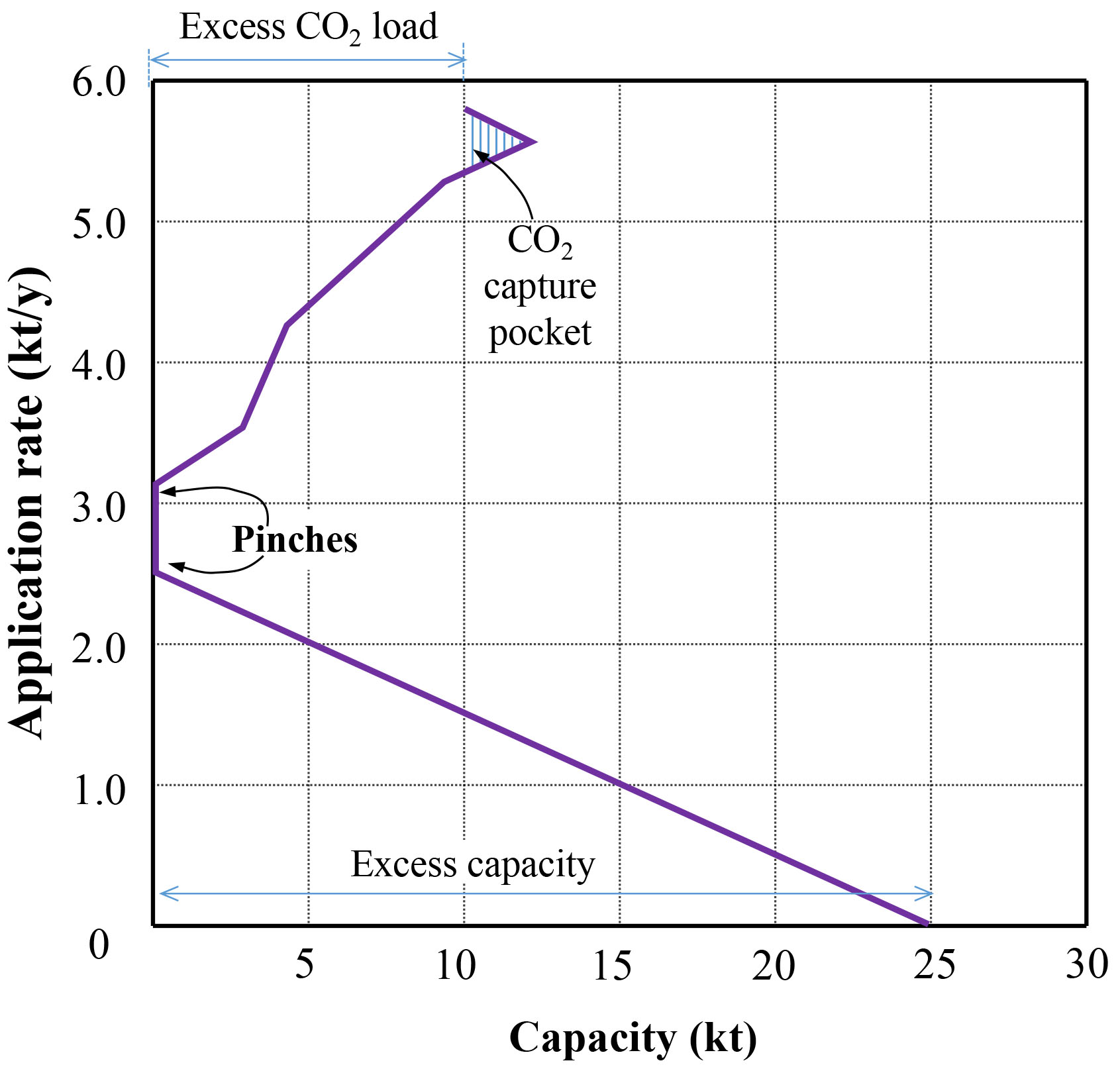
Figure 4. GCC for Example 1. GCC: Grand composite curve.
To verify the results obtained from the algebraic method, the linear programming (LP) model proposed by Tan and Aviso[29] is used to synthesise the EW network design for Example 1, as shown in Figure 5. As shown, the excess capacity of the EW problem (25 kt), and excess CO2 load (5 + 5 = 10 kt) are identical to the targeted values. Note that some important indications are necessary for this case. To cater for the capacity load of 10 kt, alternative CO2 sinks need to be developed, or the 10 kt of captured CO2 have to be sent to other alternative sinks. Alternatively, one may also reduce the captured CO2 load among the sources.
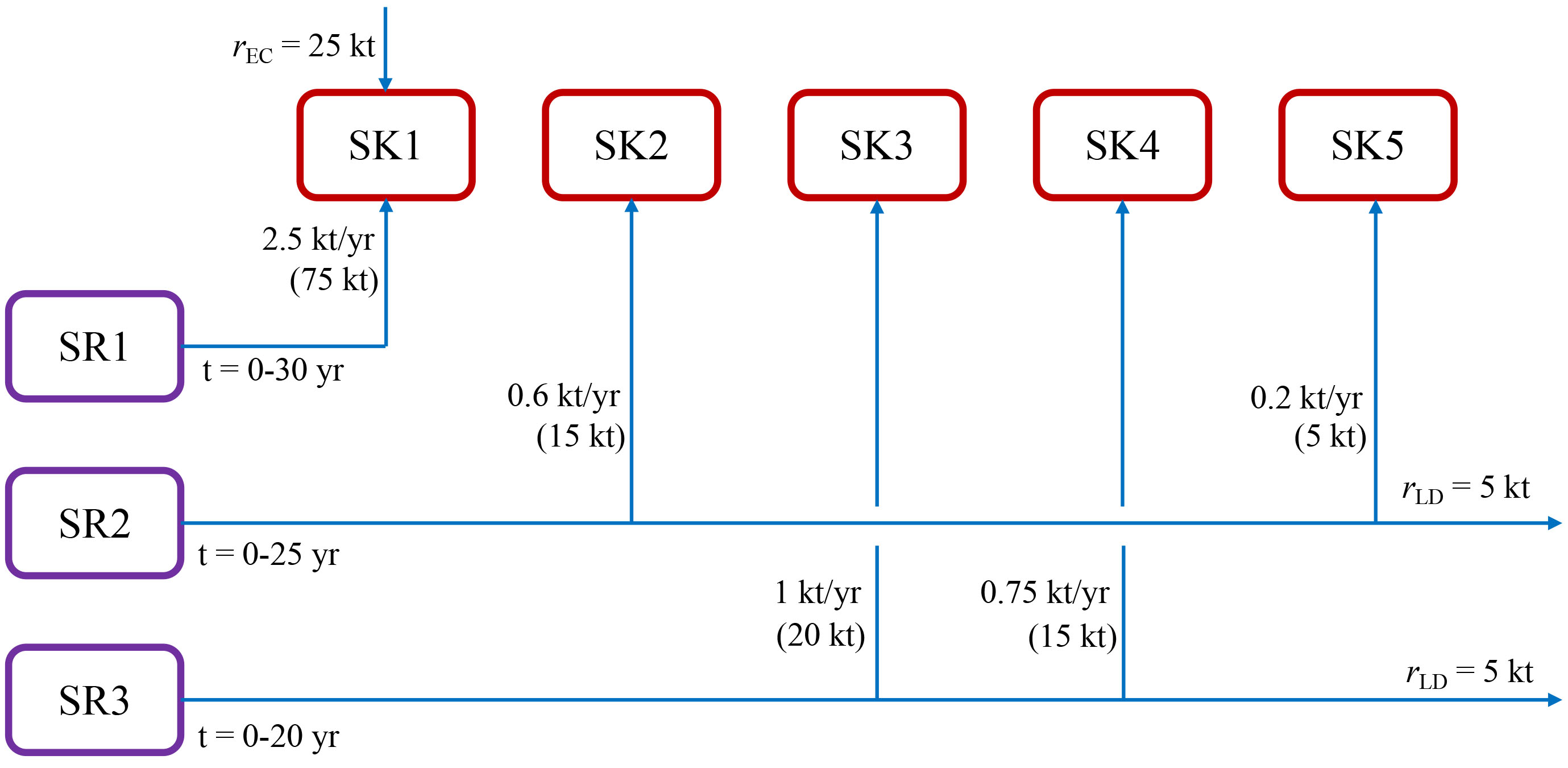
Figure 5. Optimal EW network for Example 1. EW: Enhanced weathering.
AUTOMATED TARGETING MODEL FOR EW NETWORK
The automated targeting model (ATM) was established based on pinch analysis concept but is implemented on an optimisation platform. Hence, it possesses advanced targeting capabilities over traditional CEPA approaches. In this section, the ATM is extended to the EW network, for cases involving single- and multiple-regions.
A generic framework of the ATM is given in Figure 6. As shown, the latter has a similar structure to the algebraic targeting method. Hence, Steps 1-6 of the ATM remain identical to those of the algebraic method, while its remaining steps are given as follows. Note that step 6 has different variants for EW networks of single- and multiple-region.
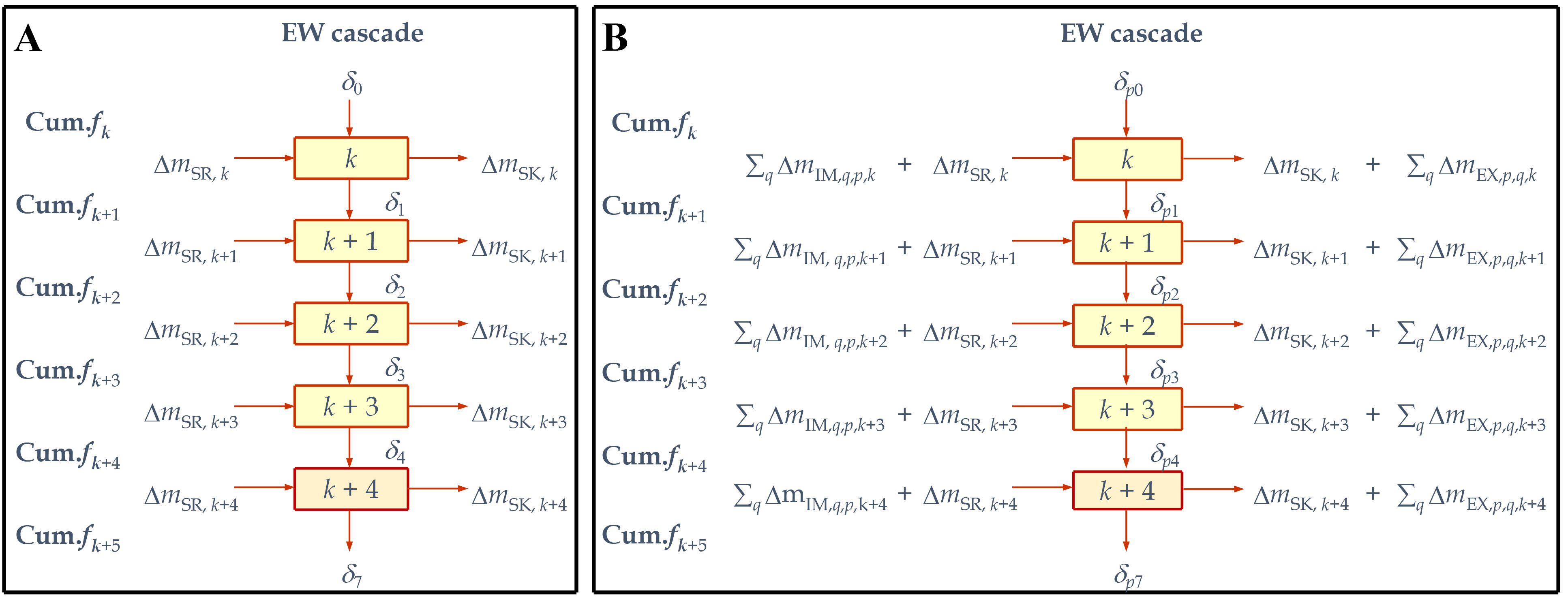
Figure 6. Generic ATM for EW for (A) a single region; (B) multiple regions. ATM: automated targeting model; EW: enhanced weathering.
7a. For EW of a single region, the residual capacity of every interval k (δk) is calculated from the net capacity between the sinks and sources, as well as the residual value cascaded from the earlier interval (δk-1), as determined using Equation 10 that follows
7b. For an EW network with multiple regions, Equation 10 is modified to consider import and export CO2 load across different regions at every interval k.
where ∆mIM,q,p,k is total CO2 load imported from region q into region p, while ∆mEX,p,q,k is total CO2 load exported from region p to region q.
8. The ATM is considered feasible when all δk values are zero or positive values, as all CO2 load flows should be non-negative values, given as in
9. Set the objective of the problem. The latter may be set to minimise the excess capacity for a single-region problem, i.e.:
For the inter-region problem, a two-stage optimisation approach may be adopted. In stage 1, the objective in Equation 13 is revised so that the overall excess capacity across all regions p is minimised:
In stage 2, the overall excess capacity determined in stage 1 is added as a new constraint as in Equation 15, while the objective is set to minimise the total cross-regional flows of CO2 load across all levels among all plants (rCP), given as in Equation 16. In practice, sending the CO2 sources to sinks in other regions indicates that CO2 emissions will be incurred from transportation. Hence, minimising cross-regional flows of CO2 load will lead to reduced transportation emissions. The main assumption here is that transportation emissions are taken as the main factor in the inter-region problem.
10. Similar to the single-region concept, the cumulative CDR for all regions (Cum TSCDR) and the total amount of rock supply from sources to sinks can be calculated using
where αp is the carbon sequestration factor for region p measured in CO2 removal per unit of crushed rock applied, βijp is the CO2 footprint per unit of crushed rock allocated from source i to sink j for region p, Rp is the total amount of rock supply from sources to sinks and, rECp and rLDp are the excess capacity and excess CO2 load of region p, respectively.
Example 2
In this hypothetical example, two different regions are considered for the EW network. These regions may represent two nearby areas that would both undergo EW implementation. In this example, the data in Table 2 (Example 1) is assumed to be region A, while data for region B is given in Table 5.
Data for region B in Example 2
| SKj | f SK j (kt/y) | t SK j (y) | m SK j (kt) | SRi | f SR i (kt/y) | t SR i (y) | m SR i (kt) | |
| 1 | 2.5 | 30 | 75 | 1 | 2 | 25 | 50 | |
| 2 | 2 | 20 | 40 | 2 | 1.5 | 20 | 30 | |
| 3 | 1 | 10 | 10 | 3 | 1 | 10 | 10 | |
| 4 | 1 | 5 | 5 | |||||
| 130 | 90 | |||||||
For comparison, ATM is first solved for the individual regions A and B. Solving the ATM with the objective in Equation 13, subject to the constraints in Equations 1-3, 10 and 12, the results are presented with EW cascades in Figure 7. As shown, region A has a total excess capacity of 25 kt, and an excess load of 10 kt [Figure 7A]; both targets are identical to those in Example 1 (see Table 4). For region B, its excess capacity was identified as 40 kt, and without any excess CO2 load [Figure 7B]. In other words, the total excess capacity is added as 65 kt (= 25 + 40 kt), and excess CO2 load is added as 10 kt (10 + 0 kt). It is also worth noting that the pinches of region A are identified as 2.5 and 3.1 kt/y, while that of region B is at the last level, i.e., 6.5 kt/y.
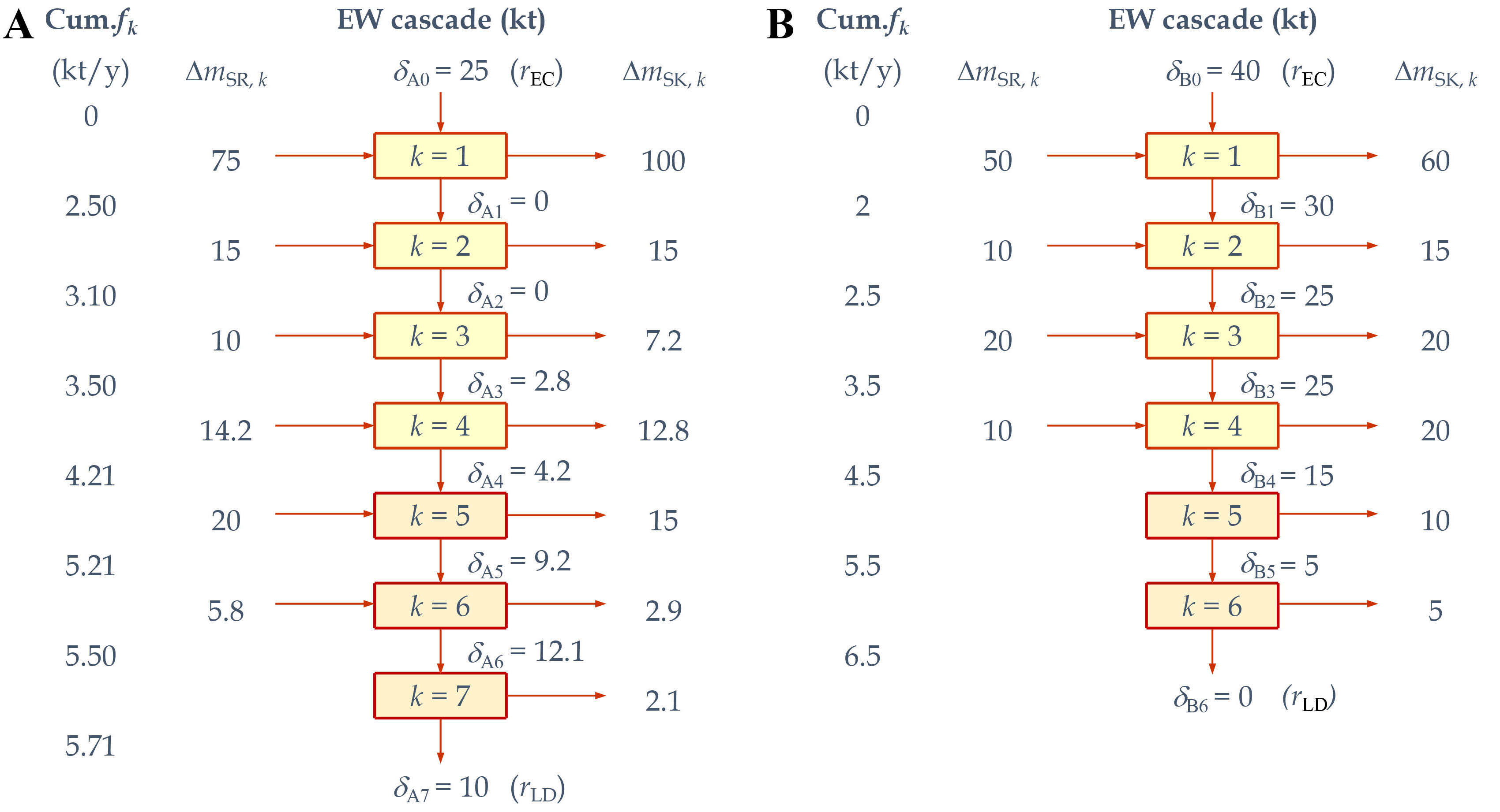
Figure 7. EW cascade for individual regions: (A) region A and (B) region B. EW: Enhanced weathering.
Next, we evaluate the potential reduction of targets when inter-regional CO2 capture will take place. This time, the ATM is solved with a two-stage optimisation approach. In stage 1, the objective in Equation 14 is solved, with constraints in Equations 1-3 and 11-12, the overall outsourced capacity is identified as 55 kt (i.e., 25 kt for region A and 30 kt for region B; see Figure 8), which is reduced by 15.4% as compared to that in Figure 7. This target is used as a new constraint as in Equation 15, while Equation 16 is used as the new objective for minimising the overall cross-regional flows. As shown in Figure 8A, the total cross-region flow is identified as 10 kt, contributed by 2.1 kt and 7.9 kt in intervals 7 and 8, respectively. Note that both of these flows indicate that basalt rock sources are sent from region A for CO2 capture in region B. Doing this leads to the removal of the excess load of region A. Figure 8 shows that both regions have zero excess load. Using Equation 18, the total amount of crushed minerals that can be supplied from the source to the sink at region A and region B are 130 kt and 100 kt, respectively. The overall TSCDR for the problem is then determined using Equation 17 as -57.5 kt [= 230 × (-0.3+0.05) kt]. Compared to individual regions [Figure 7] with total CDR of -55 kt [= (130 + 90) × (-0.3 + 0.05) kt], this corresponds to an increase of 4.5%.
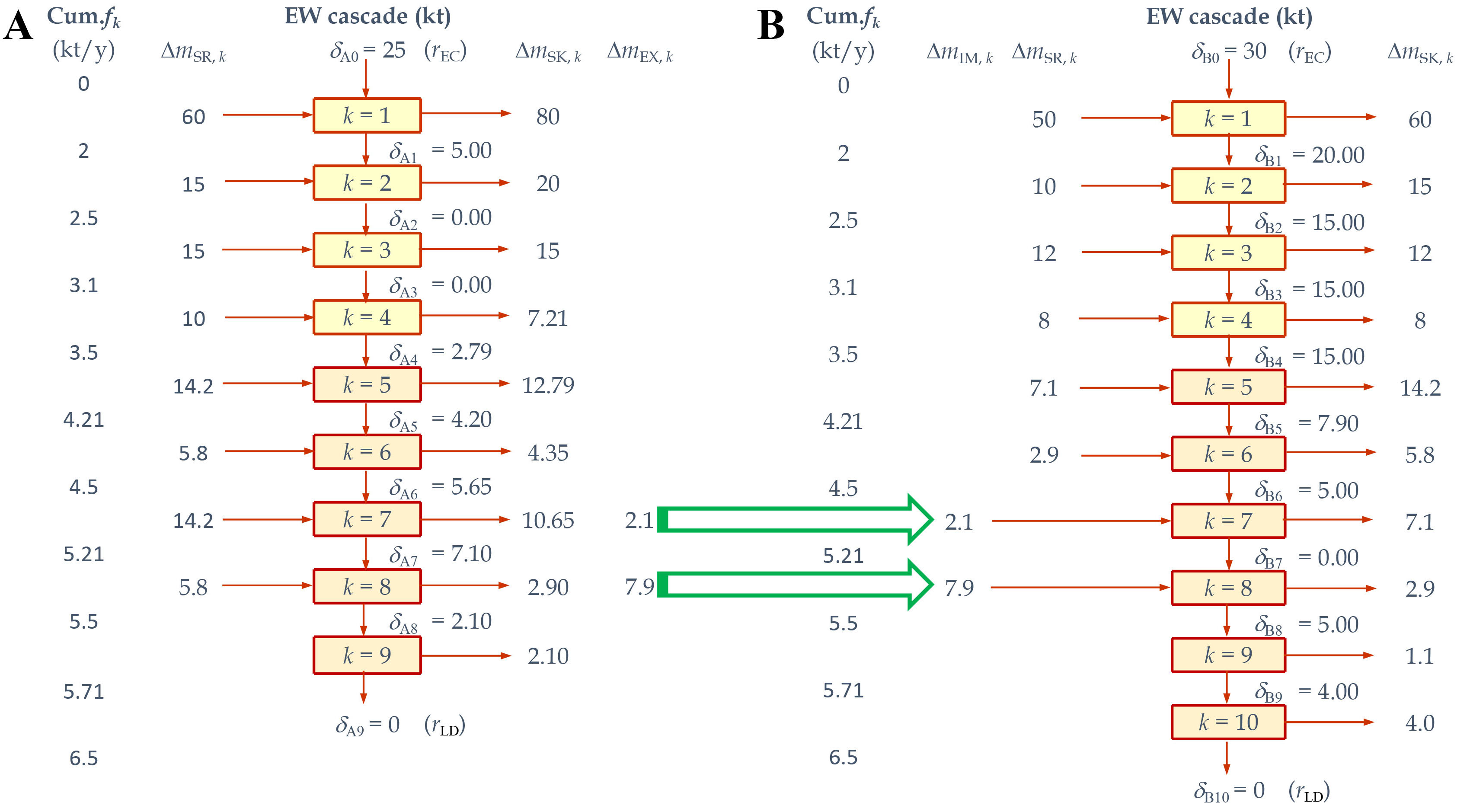
Figure 8. EW cascades for inter-regions: (A) region A; (B) region B. EW: Enhanced weathering.
Figure 9 shows the GCCs for the inter-region problem, which serves as a good visualisation tool. As shown, both regions have a new pinch, i.e., 5.71 kt/y for region A and 5.21 kt/y for region B. These pinches indicate that CO2 capture is optimised across these regions. Note that the original GCCs of the individual regions (prior to inter-region consideration) are also shown in Figure 9. It can be observed that with inter-region consideration, region B experiences reduced excess capacity (from 40 to 30 kt), while region A experiences reduced excess CO2 load (from 10 to 0 kt). Figure 10 shows the optimal EW network for the inter-regions problem, which may be synthesised using a LP model (see details in Supplementary Materials).
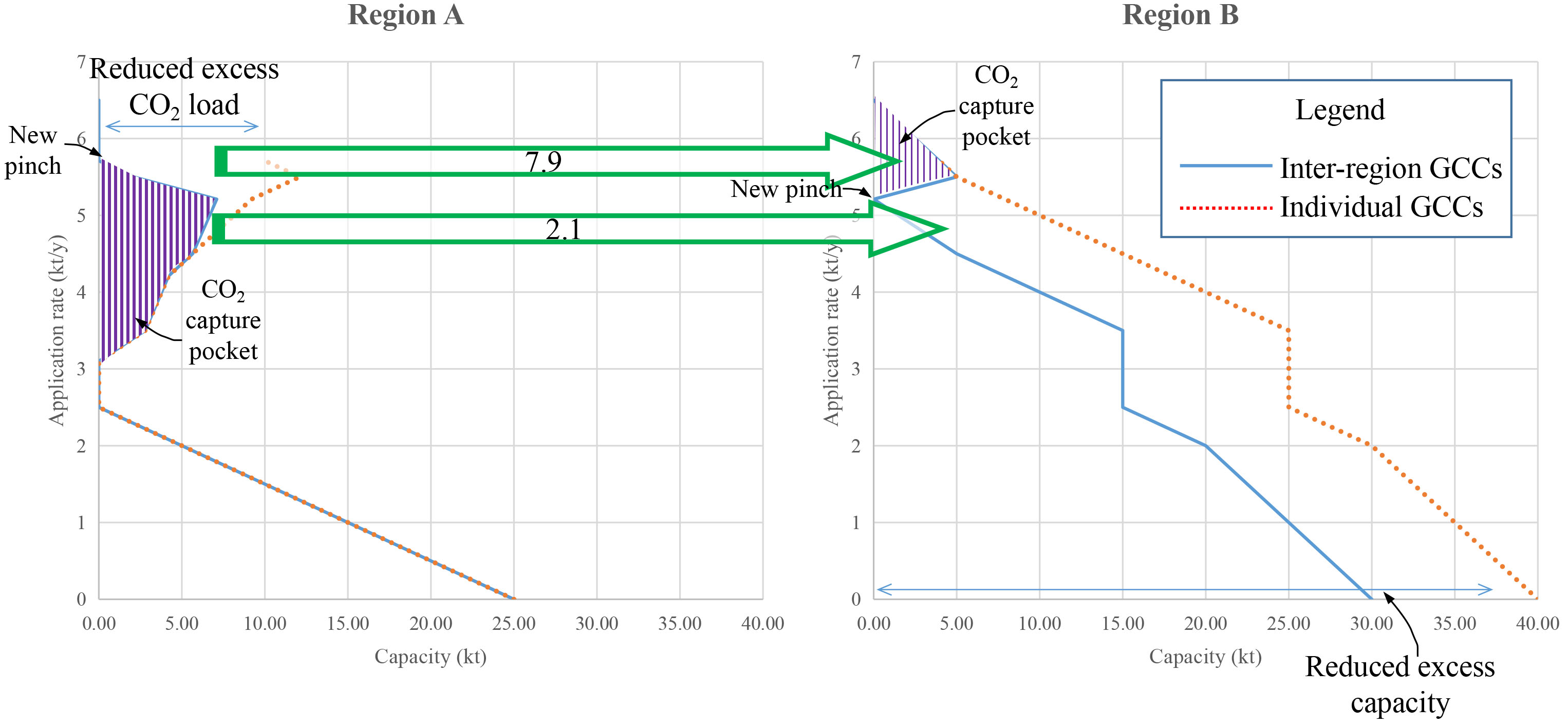
Figure 9. GCCs for the inter-region problem. GCC: Grand composite curve.
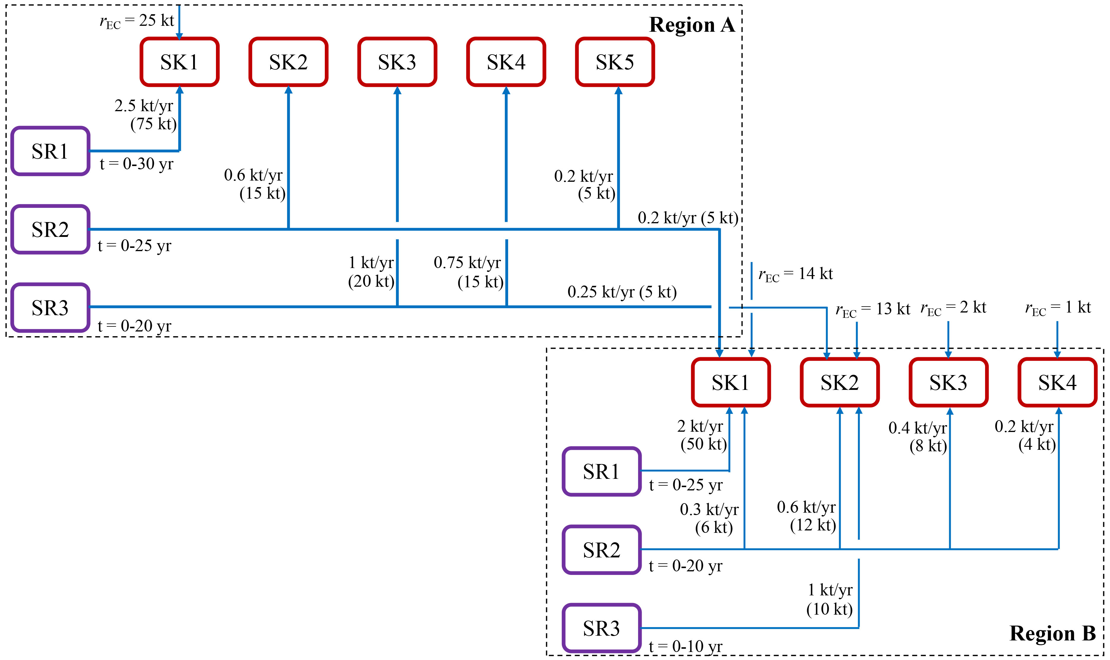
Figure 10. Optimal network design for the inter-region problem.
CONCLUSIONS
In this work, new pinch analysis tools were extended for EW problems. A new algebraic targeting tool was extended to overcome the limitation of the graphical method. Moreover, automated targeting method was extended for single- and multiple-region problems. Both tools may be used to plot the GCC, which is a useful visualisation tool for the sink-source matching problem. Two case studies, single- and multiple-region problems, were solved to elucidate the newly extended methods, along with the EW network design. Future work may focus on data uncertainties due to the risk of soil contamination in EW application. Site-specific weathering rates and process-related emissions may also be incorporated. Besides, temporal and multi-period considerations may also be incorporated.
DECLARATIONS
Authors’ contributions
Performed conception and design of the study, data analysis and interpretation: Foo, D. C. Y.
Drafted manuscript: Foo, D. C. Y.
Performed initial calculation: Woon, Z. T.; Wong, J. S.
Revised the initial draft: Tan, Y. L.
Availability of data and materials
The original contributions presented in this study are included in the article/Supplementary Materials. Further inquiries can be directed to the corresponding author.
AI and AI-assisted tools statement
Not applicable.
Financial support and sponsorship
None
Conflicts of interest
All authors declared that there are no conflicts of interest.
Ethical approval and consent to participate
Not applicable.
Consent for publication
Not applicable.
Copyright
© The Author(s) 2026.
Supplementary Materials
REFERENCES
1. EHN Curators. Earth is now expected to cross 1.5 °C warming by 2027, WMO Warns. 2025. www.ehn.org [accessed 2026-9-16].
2. Intergovernmental Panel on Climate Change. Chapter 11: Weather and climate extreme events in a changing climate. In Climate Change 2021: The Physical Science Basis; Cambridge University Press, 2021. https://www.ipcc.ch/report/ar6/wg1/chapter/chapter-11/ [accessed 2026-9-16].
3. Allen, M. R.; Dube, O. P.; Solecki, W.; et al. Framing and context. In Global Warming of 1.5 °C; IPCC, 2018.
4. Mcglashan, N.; Shah, N.; Caldecott, B.; Workman, M. High-level techno-economic assessment of negative emissions technologies. Process. Saf. Environ. 2012, 90, 501-10.
5. Holbrow, P. Dust explosion venting of small vessels and flameless venting. Process. Saf. Environ. 2013, 91, 183-90.
6. Tan, R. R.; Foo, D. C. Pinch analysis approach to carbon-constrained energy sector planning. Energy 2007, 32, 1422-9.
7. Linnhoff, B.; Townsend, D. W.; Boland, D.; et al. A user guide on process integration for the efficient use of energy; IChemE: Rugby, 1994. https://archive.org/details/userguideonproce0000unse.
8. Smith, R. Chemical process: design and integration, 2nd ed.; John Wiley & Sons: West Sussex, England/New York, 2016. wiley.com/en-kr/Chemical+Process+Design+and+Integration,+2nd+Edition-p-9781119990147.
9. El-Halwagi, M. M. Sustainable design through process integration, 2nd ed.; Butterworth-Heinemann, 2017.
11. Ramsook, D.; Boodlal, D.; Maharaj, R. Optimizing carbon reduction strategies in Trinidad and Tobago’s power generation sector: insights from carbon emission pinch analysis. Carbon. Manage. 2025, 16, 2523917.
12. Ramsook, D.; Boodlal, D.; Maharaj, R. Multi-period carbon emission pinch analysis (CEPA) for reducing emissions in the Trinidad and Tobago power generation sector. Carbon. Manage. 2022, 13, 164-77.
13. Crilly, D.; Zhelev, T. Emissions targeting and planning: An application of CO2 emissions pinch analysis (CEPA) to the Irish electricity generation sector. Energy 2008, 33, 1498-507.
14. Crilly, D.; Zhelev, T. Further emissions and energy targeting: an application of CO2 emissions pinch analysis to the Irish electricity generation sector. Clean. Techn. Environ. Policy. 2010, 12, 177-89.
15. Su, W.; Ye, Y.; Zhang, C.; Baležentis, T.; Štreimikienė, D. Sustainable energy development in the major power-generating countries of the European Union: the pinch analysis. J. Clean. Prod. 2020, 256, 120696.
16. Cossutta, M.; Foo, D. C.; Tan, R. R. Carbon emission pinch analysis (CEPA) for planning the decarbonization of the UK power sector. Sustainable. Prod. Consumption. 2021, 25, 259-70.
17. Poplewski, G.; Ting, M.; Foo, D. C. Y.; Tan, R. R.; Tan, Y. L. Carbon emission pinch analysis for transformation of Polish power generation sector. Clean. Techn. Environ. Policy. 2025, 27, 4685-709.
18. Cao, J.; Jia, X.; Wang, F. Projection of energy mix in China using carbon emission pinch analysis. IOP. Conf. Ser:. Earth. Environ. Sci. 2021, 821, 012013.
19. Rajakal, J. P.; Saleem, N. N.; Wan, Y. K.; Ng, D. K. S.; Andiappan, V. Low-carbon energy transition for the Sarawak region via multi-period carbon emission pinch analysis. Processes 2023, 11, 1441.
20. Tarequzzaman, M.; Khan, I.; Sahabuddin, M.; Al-Amin, M. Strategic pathways to sustainable energy: carbon emission pinch analysis for Bangladesh’s electricity sector. J. Renew. Sustain. Ener. 2024, 16, 025904.
21. Atkins, M. J.; Morrison, A. S.; Walmsley, M. R. Carbon Emissions Pinch Analysis (CEPA) for emissions reduction in the New Zealand electricity sector. Applied. Energy. 2010, 87, 982-7.
22. Walmsley, M. R.; Walmsley, T. G.; Atkins, M. J.; Kamp, P. J.; Neale, J. R. Minimising carbon emissions and energy expended for electricity generation in New Zealand through to 2050. Applied. Energy. 2014, 135, 656-65.
23. Tan, R. R.; Aviso, K. B.; Bandyopadhyay, S. Pinch-based planning of terrestrial carbon management networks. Clean. Eng. Technol. 2021, 4, 100141.
24. Mu, P.; Yang, Y.; Han, Y.; Gu, X.; Zhu, Q. Raw material management networks based on an improved P‐graph integrated carbon emission pinch analysis (CEPA‐P‐graph) method. Can. J. Chem. Eng. 2020, 98, 676-89.
25. Zhang, Y.; Wang, H.; Zhou, T.; Li, Z.; Jia, X. Extended carbon emission pinch analysis for the low-carbon tobacco industry. Energies 2022, 15, 4611.
26. Chew, Z. T.; Hoy, Z. X.; Woon, K. S.; Liew, P. Y. Integrating greenhouse gas reduction and waste policy targets to identify optimal waste treatment configurations via carbon emission pinch analysis. Process. Saf. Environ. 2022, 160, 661-75.
27. Yang, D.; Qin, Y.; Xu, Y.; et al. Sequestration of carbon dioxide from the atmosphere in coastal ecosystems: Quantification, analysis, and planning. Sustainable. Prod. Consumption. 2024, 47, 413-24.
28. Goll, D. S.; Ciais, P.; Amann, T.; et al. Potential CO2 removal from enhanced weathering by ecosystem responses to powdered rock. Nat. Geosci. 2021, 14, 545-9.
Cite This Article
 Open Access
How to Cite
Foo, D. C. Y.; Woon, Z. T.; Wong, J. S.; Tan, Y. L. Algebraic and automated targeting for inter-region problems in terrestrial carbon management network. Carbon Footprints 2026, 5, 51. https://dx.doi.org/10.20517/cf.2026.18
Download Citation
If you have the appropriate software installed, you can download article citation data to the citation manager of your choice. Simply select your manager software from the list below and click on download.
Export Citation File
Type of Import
Tips on Downloading Citation
Citation Manager File Format
Type of Import
Direct Import: When the Direct Import option is selected (the default state), a dialogue box will give you the option to Save or Open the downloaded citation data. Choosing Open will either launch your citation manager or give you a choice of applications with which to use the metadata. The Save option saves the file locally for later use.
Indirect Import: When the Indirect Import option is selected, the metadata is displayed and may be copied and pasted as needed.
About This Article
Copyright

Data & Comments
Data
0












Comments
Comments must be written in English. Spam, offensive content, impersonation, and private information will not be permitted. If any comment is reported and identified as inappropriate content by OAE staff, the comment will be removed without notice. If you have any queries or need any help, please contact us at [email protected].