


The uncertainty of using carbon footprint as a predictor of overall environmental impacts: comparing linear, logarithmic and circular methods
 0
0 
Abstract
The carbon footprint (CF) is widely used as a proxy indicator for the overall environmental impacts of entities such as countries, organizations, and products. However, since CF is by definition limited to greenhouse gas emissions, an important question arises: to what extent is CF a reliable predictor of other environmental impacts, including ozone layer depletion, acidification, eutrophication, and toxicity? This question has been examined in previous studies, yielding mixed results. In this paper, we argue that the analytical methods employed in earlier work may lead to misleading conclusions. We therefore propose the use of methods from directional statistics as an alternative approach. We analyze the correlation between life-cycle environmental impacts across approximately 4,000 products using a range of metrics, including linear, logarithmic, and rank-based regression, as well as directional statistics-based measures. Our findings are consistently negative: CF does not serve as a reliable predictor for any of the other environmental impact categories considered. Moreover, we show that traditional metrics used to assess such relationships can be misleading. Overall, relying on CF as a measure of total environmental burden is likely to introduce substantial uncertainty, even in cases where conventional correlation indicators suggest otherwise.
Keywords
INTRODUCTION
The growing societal concern over climate change has stimulated widespread interest in the application of the carbon footprint (CF). When applied to products, CF quantifies greenhouse gas (GHG) emissions across the entire life cycle, from resource extraction to recycling and disposal[1]. However, using CF as the sole basis for decision-making risks favoring technologies or products that may impose greater environmental burdens in other impact categories, thereby leading to problem shifting[2,3].
At the same time, the rise of CF presents an opportunity to assess environmental impacts more broadly. GHG emissions are generally easier to inventory and estimate than many other pollutants, such as PM2.5, nitrates, or pesticides. Moreover, the characterization of their impacts through global warming potentials benefits from a well-established, consensus-driven scientific foundation, particularly through the work of the Intergovernmental Panel on Climate Change. In addition, GHG emissions are increasingly subject to stringent regulatory reporting requirements[4]. Collectively, these factors make it more straightforward to quantify GHG emissions and their impacts than to assess effects such as respiratory damage from particulate matter, eutrophication, or ecotoxicity. In this context, CF has been proposed as a potential proxy indicator for overall environmental impact[5].
To evaluate this proposition, researchers have investigated the extent to which CF can serve as an indicator of overall environmental impact. Prior studies have typically examined the relationship between CF and other environmental impact indicators across samples of products and subsequently generalized the findings. Examples include[4,5], and[6]. These studies follow an approach originally established in[7] and[8], with numerous subsequent contributions[9-13], in which correlations between impact categories are analyzed in a quasi-empirical manner, often with the aim of identifying proxy indicators.
The results of these studies are mixed. For example[14], concludes that “resource footprints are good proxies of environmental damage”, as they “accounted for > 90% of the variation in the damage footprints”. In contrast[6], finds that “some environmental impacts, notably those related to emissions of toxic substances, often do not covary with climate change impacts”, and therefore argues that “carbon footprint is a poor representative of the environmental burden of products”.
Despite their insights, these studies are subject to a methodological limitation: their reliance on correlation analysis. While correlation analysis is appropriate in certain contexts, it may be unsuitable for assessing the consistency between competing life cycle assessment (LCA) methods based on product samples[15]. A key issue is its sensitivity to the choice of functional unit. For instance, the impact associated with 1 kg of concrete will differ from that of 1 m3 of concrete, and such changes in scale can alter both correlation and regression outcomes. This issue is discussed in more detail in a later section.
As an alternative[15], propose the use of directional (or circular) statistics[16,17], illustrated through a relatively simple case study. However, the question of predictive performance remains largely unexplored. In this study, we revisit the question of whether CF can serve as a proxy for overall environmental impact using directional statistics, drawing on an extensive dataset from[6] comprising approximately 4,000 products. We compare the results with those obtained from linear and logarithmic regression models. Unlike most prior work, we examine not only overall model fit but also predictive performance for subsets of individual products.
This paper does not aim to reassess the validity of CF using a new or expanded dataset. Instead, it advances the following hypotheses:
• conventional analyses based on correlation and/or regression are not well-suited to this research question;
• directional statistics provide a more appropriate analytical framework;
• standard reporting practices that emphasize aggregate fit obscure the associated increase in uncertainty;
• a new uncertainty metric, the normalized residual, better captures this aspect.
Given this focus, we do not present a comprehensive literature review but instead draw on representative studies to illustrate prevailing analytical approaches. We reuse the dataset from[6] without modification, as it remains one of the largest and most widely cited datasets in this domain, thereby enabling direct comparison with previously reported results.
The remainder of the paper is structured as follows. First, we describe the applied methods (correlation analysis, regression analysis, and directional statistics) and explain why correlation-based approaches may yield misleading conclusions for this research question. We then present results based on directional statistics, followed by a discussion of their implications.
METHODS AND DATA
Correlation and regression analysis
Because correlation and regression are well-established methods, we do not provide a full methodological description and instead refer to standard texts, such as[18] and[19]. Nonetheless, a brief recap is warranted, particularly because some previous studies (e.g., [8]) conflate correlation and regression, for example, by interpreting R2 as a measure of correlation (see[20] for a detailed discussion).
The sample version of the Pearson correlation coefficient, denoted r, quantifies the strength of the linear association between two numerical variables. It is calculated as
where xi and yi are the values of the two variables (e.g., CF and toxicity) for product i, and
The Spearman rank correlation coefficient, ρ. is computed using the ranks of the data. Denoting by x(i) the rank of xi within the vector x, one defines
where
Both r and ρ are bounded between [-1,1]. Values of r = 1 and -1 indicate a perfect positive or negative linear relationship, respectively, whereas ρ = 1 or -1 indicates a perfect positive or negative monotonic relationship, which need not be linear. Both coefficients are symmetric (i.e., swapping x and y does not change their value) and are invariant under changes of units or scale, for example, expressing CF in kilograms versus tonnes of CO2-eq does not affect the results.
Regression analysis, in contrast, assumes a causal relationship between variables. Here, we focus on simple linear regression:
where a and b are the regression coefficients, and ei is the residual for observation i. The slope b is estimated as
and the constant (or intercept) a by
The quality of the regression fit is typically measured by the coefficient of determination, R2:
R2 ranges from 0 to 1, and represents the proportion of variance in y explained by x. A value of R2 = 1 indicates perfect prediction of yi from xi, whereas R2 = 0 indicates no predictive power. Further details on prediction methods are provided in the next section.
For a given regression model, it holds that the coefficient of determination is equal to the squared Pearson correlation coefficient:
However, R2 should not be interpreted as a correlation coefficient or “squared correlation”, as is sometimes suggested in the literature. Correlation quantifies the strength of association between two variables in a symmetric manner, without assuming causality. Regression, by contrast, is asymmetric: the estimated coefficients a and b change if the roles of x and y are reversed, reflecting the underlying assumption that one variable predicts or explains the other. Unlike correlation, regression is explicitly intended for predictive purposes. Therefore, while correlation analysis can indicate whether a predictive relationship may exist, it cannot be used to make predictions. Studying the potential of CF as a predictor of other environmental impacts thus requires a regression framework rather than correlation alone.
Prediction with regression analysis
Thus far, the discussion has focused on evaluating the strength of the relationship between CF and other impact indicators across a large sample of products. A more practical question, however, is how to predict the value of a second impact indicator for a specific product when its CF is known. If the goal is to use CF as a predictor, the prediction procedure itself must be explicitly defined.
Perhaps surprisingly, previous studies such as[4] and[5] do not address this issue. They report summary statistics, e.g., Pearson’s r, Spearman’s ρ, the coefficient of determination (R2), or other measures of overall association, but these metrics alone do not enable prediction. For example, knowing that a product has a CF of 12 and that the global correlation between CF and toxicity yields R2 = 0.78 does not allow one to determine the toxicity score for that product. To make such predictions, a regression model is required, such as
where a and b are estimated regression coefficients and
Linear and logarithmic relations
When analyzing a sample of products, as in[4-14], large differences in the magnitude of variables are common. For example, in[6], the CF axis spans from 10-12 to 108. On a linear scale, most data points would be compressed into a tiny region, making visualization difficult and potentially affecting correlation and regression analyses. For this reason, logarithmic transformations are often applied. However, it is not always clear whether logarithms are used solely for plotting or also in the statistical calculations. For instance, [6] and [8] indicate “logarithmic scales” in figure captions but do not clarify whether the analyses were performed on transformed variables.
Applying a logarithm to both variables entails analyzing x’ = log(x) and y’ = log(y). This transformation can substantially affect Pearson’s r, the regression coefficients a amd b, and the coefficient of determination R2. In contrast, Spearman’s rank correlation ρ remains unaffected because the logarithm is monotonic. Care is required, however, as logarithms are defined only for positive values. Excluding non-positive data points may alter ρ if these points are removed from the sample.
The base z of the logarithm is not critical. Since
Prediction using a logarithmic transformation proceeds as follows. We consider the natural logarithm for illustration. The regression model on the transformed variables is
where x’ = ln(xi) and y’ = ln(yi), and a’ and b’ are the regression coefficients estimated from the log-transformed data. The predicted value of yi on the original scale is then
where a” = exp(a’). This form makes explicit the power-law relationship between the original variables implied by logarithmic regression.
Fallacy of correlation and regression analysis
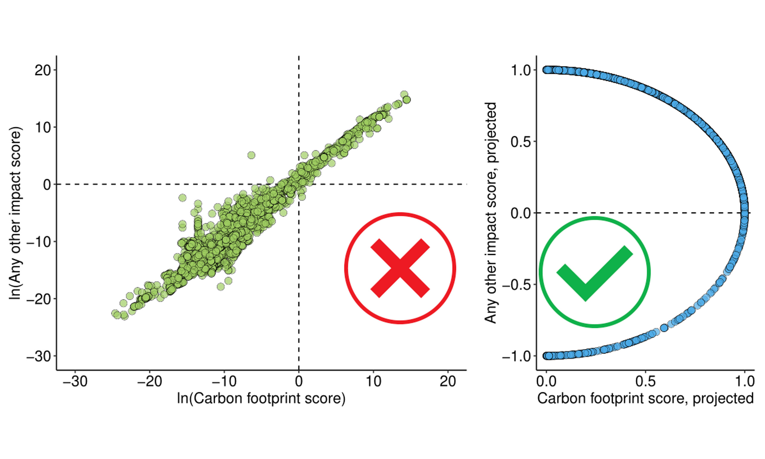
[6] analyzed the suitability of using CF as a proxy for multiple impact categories based on a sample of 3,953 products. Their analysis relied on correlation measures, which [15] have shown to be vulnerable to methodological limitations. The primary issue is that each data point (xi,yi) has an essentially arbitrary scale: it could be rescaled to (cxi,cyi) for any c
Figure 1 illustrates this issue using a small sample of four points. Three points are fixed (green circles), while the fourth (red square) is rescaled by factors of c = 0.1 in Figure 1B and c = 10 in Figure 1C, producing dramatic changes in the correlation statistics.
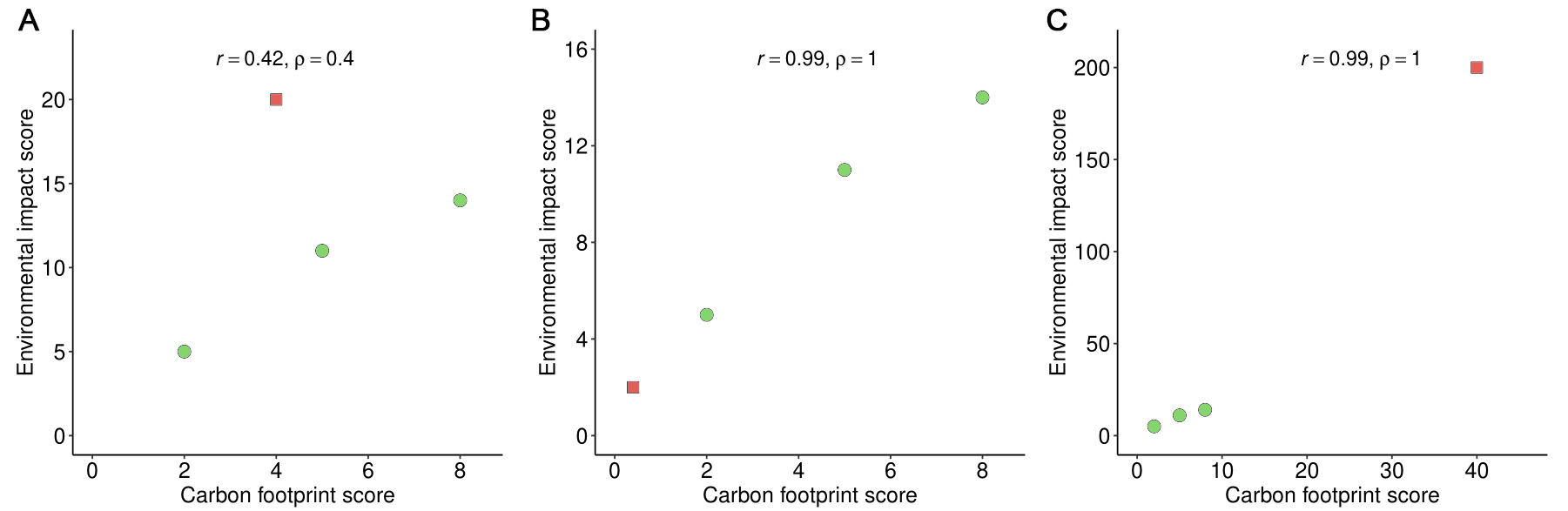
Figure 1. (A) Four data points yield a weak correlation; (B) Rescaling the red square data point by a factor of 0.1 produces a strong correlation; (C) Rescaling the same data point by a factor of 10 also results in a strong correlation. The Pearson correlation coefficient is denoted r, and the Spearman rank correlation coefficient is denoted ρ.
Directional statistics
The issue described in the previous section can be addressed by analyzing the ratio between the two variables for each data point:
This ratio is insensitive to changes in scale. If the k-values across the sample are relatively uniform, x serves as a good proxy for y. Conversely, a wide variation in k-values indicates that x is a poor predictor of y. In the example of Figure 1, the k-values are 2.5, 1.75, 2.2, and 5, showing substantial variation, consistent with Figure 1A. This variation, however, is obscured in Figure 1B and C, and is not reflected in the correlation coefficients (r = 0.99, ρ = 1).
Using k-values to calculate averages or standard deviations is not recommended, because the division by x produces highly non-linear behavior when the slope is steep. A more robust approach is to convert the ratio into an angle using the inverse tangent function:
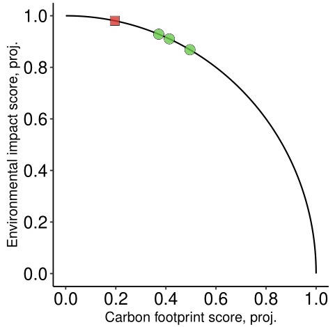
For the data points in Figure 1, the resulting angles are 1.19, 1.05, 1.14, and 1.37 radians. These angles can be visualized by projecting the points onto the unit circle, as illustrated in Figure 2.
These projected points can be analyzed using directional statistics. The average slope is computed as
and the corresponding mean resultant length is
In directional statistics ([16,17]), the circular variance V is a standard measure of dispersion, providing a robust indicator of the consistency of the slope across the sample:
The circular variance V ranges between 0 and 1. A value of V = 0 indicates that x is a perfect predictor of y, whereas V = 1 corresponds to a complete lack of predictive value. When the analysis is restricted to the first quadrant (i.e., assuming both x and y are non-negative), a uniformly dispersed set of data points yields an average angle
An additional issue concerns the treatment of observations across different quadrants. Consider a dataset consisting of two points, (2,3) and (-2,-3), which lie in the first and third quadrants, respectively. Intuitively, these points should cancel out, yielding a mean resultant length of zero. However, using the single-argument inverse tangent function (ATAN) yields identical angles, since
Prediction with directional statistics
The mean angle
yielding a predicted value
Traditionally, prediction error is quantified using the residual ei = yi -
To address these issues, we define the normalized residual fi as
This measure is scale-invariant and treats over- and underestimation symmetrically in relative terms. Although introduced in the context of directional statistics, the normalized residual can equally be applied to predictions obtained from conventional regression models.
Fallacies of predicting with regression
An instructive situation arises when the amount of product under analysis is rescaled. Suppose the CF of 1 kg of a product is x, and the corresponding value of another impact category is y. If we instead consider 1,000 kg of the same product, these values scale proportionally to 1000x 1000y. A consistent prediction method should therefore yield a predicted value
To assess this property, we examine the ratio between the prediction for 1,000 units and that for 1 unit. For linear regression, this ratio is
which is generally not equal to 1000, except in the special case where a = 0.
For logarithmic regression, the ratio becomes
which simplifies to 1000b, and thus equals 1000 only if b = 1.
For the circular method, the ratio is
which is exactly 1000 (provided
A second relevant case concerns vanishing product quantities. As x → 0, the true impact y also approaches zero. However, under linear regression,
These observations demonstrate that prediction of one impact indicator from another, specifically, predicting environmental impacts from CF, is structurally more consistent with directional statistics than with conventional regression approaches.
Data
We used the dataset of 3,953 products originally analyzed in [6], which includes values for the carbon footprint as well as a range of additional environmental impact categories (see Table 1 for an overview).
Summary statistics of the association between the carbon footprint (CF) and a range of environmental impact categories, based on a sample of 3,953 products
| Impact category | Pearson r (linear) | Pearson r (logarithmic) | Spearman ρ (linear and logarithmic) | Circular variance V |
| Ozone depletion | 0.99 | 0.96 | 0.75 | 0.016 |
| Ozone formation (vegetation) | 0.97 | 0.99 | 0.80 | 0.094 |
| Ozone formation (human) | 0.97 | 0.99 | 0.80 | 0.112 |
| Acidification | 0.96 | 0.98 | 0.79 | 0.140 |
| Terrestrial eutrophication | 0.94 | 0.98 | 0.75 | 0.093 |
| Aquatic eutrophication EP (N) | 0.95 | 0.98 | 0.72 | 0.089 |
| Aquatic eutrophication EP (P) | 0.84 | 0.95 | 0.73 | 0.200 |
| Ecotoxicity water chronic | 0.96 | 0.97 | 0.80 | 0.041 |
| Ecotoxicity water acute | 0.93 | 0.96 | 0.80 | 0.023 |
| Ecotoxicity soil chronic | 0.96 | 0.94 | 0.67 | 0.035 |
| Ecotoxicity freshwater | 0.92 | 0.96 | 0.76 | 0.164 |
| Human toxicity (non-carc) | 0.85 | 0.96 | 0.74 | 0.180 |
| Human toxicity (carc) | 0.9 | 0.97 | 0.78 | 0.176 |
| Respiratory ìnorganics | 0.98 | 0.97 | 0.75 | 0.141 |
| Land use | 0.10 | 0.96 | 0.63 | 0.056 |
| Resource depletion | 0.92 | 0.96 | 0.77 | 0.177 |
For each impact category, we computed the Pearson correlation coefficient (r) for both the original data and log-transformed data, the Spearman rank correlation coefficient (ρ), and the directional statistic, expressed as the circular variance (V).
To evaluate predictive performance, we selected a set of representative products spanning different categories:
• 1-pentanol, at plant (1 kg, region RER)
• aluminium, production mix, at plant (1 kg, region RER)
• barge tanker (1 piece, region RER)
• electricity mix (1 MJ, region DE)
• operation, average train (1 person-km, region DE)
• potatoes, at farm (1 kg, region US)
For each of these six products, the acidification impact was estimated using three prediction methods: linear regression, logarithmic regression, and directional statistics. The predicted values were then compared to the observed values using the normalized residual as a measure of prediction error.
RESULTS
Overall quality of fit
The main results are summarized in Table 1.
The results reveal several inconsistencies across metrics. For example, acidification exhibits strong correlation statistics, yet performs among the worst when evaluated using directional statistics. Conversely, land use shows a relatively low Pearson correlation coefficient but ranks among the best according to circular variance. It should be noted that the linear and logarithmic Pearson coefficients, as well as the non-parametric Spearman coefficient, are derived from methods that we have argued to be theoretically inappropriate for this research question. The discrepancies observed here therefore underscore that our critique is not merely theoretical but also has clear empirical implications.
To facilitate interpretation, selected results are visualized. Figure 3 presents the case of ozone depletion. On a linear scale [Figure 3A], a clear positive association is apparent, with higher values of x corresponding to higher values of y. On a logarithmic scale [Figure 3B], the association remains visible, although a number of data points deviate from the general pattern. The circular representation [Figure 3C] provides additional insight. While the first quadrant (positive x and y) is densely populated, the points are widely dispersed within this quadrant, without a clear concentration. The resulting circular variance is 0.02, indicating poor suitability as a proxy. In addition, the fourth quadrant contains a non-negligible number of observations: approximately 10% of products exhibit a negative CF while maintaining non-negative ozone depletion scores, further weakening predictive performance.
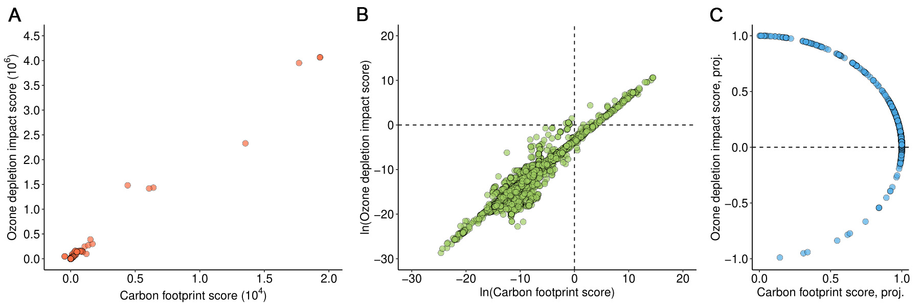
Figure 3. Scatterplots of the carbon footprint (horizontal axis) versus ozone depletion impact (vertical axis) for the product sample. Panel (A) shows both axes on a linear scale; panel (B) uses logarithmic scales; panel (C) presents the data projected onto the unit circle (“proj.”).
Although ozone depletion represents one of the better-performing impact categories, aquatic eutrophication [EP (P)] is among the worst. The corresponding results are shown in Figure 4.
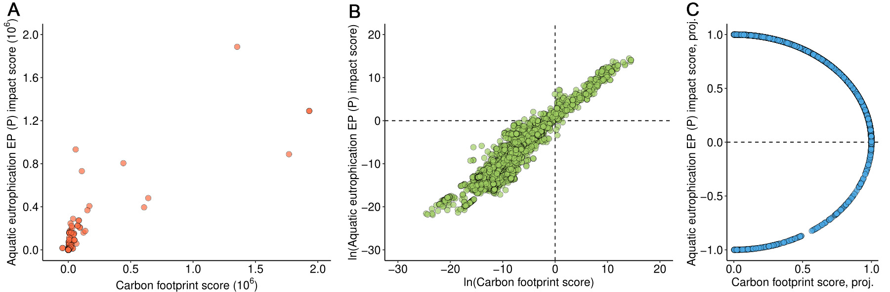
Figure 4. Scatterplots of the carbon footprint (horizontal axis) versus aquatic eutrophication EP (P) impact (vertical axis) for the product sample. Panel (A) shows both axes on a linear scale; panel (B) uses logarithmic scales; panel (C) presents the data projected onto the unit circle (“proj.”).
In the original analysis by [6], the Spearman correlation coefficient was used, yielding values “between 0.7 and 0.8 for all impact categories except land use”, which “suggests a good correlation between CF ... and the rest of the environmental impact scores”. [6] further reports that the Spearman correlation coefficients are associated with “P < 0.05”. This likely refers to a hypothesis test of the null hypothesis of no correlation (ρ = 0), which is rejected at the 95% confidence level. While this may appear compelling, such significance is largely driven by the large sample size. With n = 3,953, even a very weak correlation (e.g., ρ ≈ 0.03) will be deemed statistically significant. As a result, statistical significance in this context provides limited information about the practical strength or relevance of the association]. In contrast, the directional statistical analysis presented here leads to a markedly different conclusion. All circular variance values are 0.02 or higher, and the patterns observed in Figures 3C and 4C reveal substantial dispersion.
In a subsequent refinement, [6] qualifies its initial conclusions by noting that energy-related products exhibit lower correlations (“below 0.7”), whereas infrastructure-related products show higher correlations (“above 0.94 for all impact categories”). This prompted us to revisit the case of infrastructure products using directional statistics. The results are shown in Figure 5.
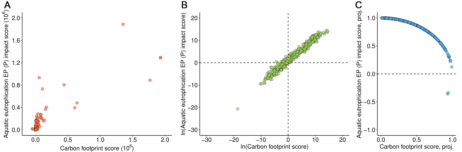
Figure 5. Scatterplots of the carbon footprint (horizontal axis) versus aquatic eutrophication EP (P) impact (vertical axis) for 488 infrastructure-related products. Panel (A) shows both axes on a linear scale; panel (B) uses logarithmic scales; panel (C) presents the data projected onto the unit circle (“proj.”).
While the Spearman correlation remains high (0.96), the directional analysis provides a more nuanced perspective. Although most observations lie in the first quadrant, they remain widely dispersed within it, resulting in a circular variance of 0.05. This value exceeds the proposed threshold of 0.001 by a factor of 50, indicating poor predictive performance despite the high correlation coefficient.
Predicted values
Table 2 presents the acidification scores alongside their predicted values obtained using three methods: linear regression, logarithmic regression, and directional statistics, for six representative products (see Section 2.8 for details).
Acidification scores and corresponding predictions using three methods
| Product | True score | Linear prediction | Logarithmic prediction | Circular prediction |
| i | yi | | | |
| 1-pentanol | 5.19 · 10-4 | 8.76 · 102 | 9.11 · 10-4 | 5.73 · 10-4 |
| Aluminium | 1.70 · 10-3 | 8.76 · 102 | 1.73 · 10-3 | 1.01 · 10-3 |
| Barge tanker | 2.18 · 102 | 1.02 · 103 | 2.20 · 102 | 1.16 · 102 |
| Electricity | 1.07 · 10-5 | 8.76 · 102 | 3.46 · 10-5 | 2.10 · 10-5 |
| Train transport | 7.59 · 10-6 | 8.76 · 102 | 1.32 · 10-6 | 8.00 · 10-6 |
| Potatoes | 5.47 · 10-5 | 8.76 · 102 | NA | -2.12 · 10-5 |
Table 3 reports the corresponding normalized (relative) residuals for these predictions.
Normalized residuals for the acidification impact of selected products, based on three prediction methods
| Product | Linear residual | Logarithmic residual | Circular residual |
| i | fi (%) | fi (%) | fi (%) |
| 1-pentanol | -1.7 · 108 | -75 | -3 |
| Aluminium | -5.1 · 107 | -1 | 41 |
| Barge tanker | -366 | -1 | 47 |
| Electricity | -8.1 · 109 | -223 | -96 |
| Train transport | -1.1 · 1010 | -72 | -5 |
| Potatoes | -1.6 · 109 | NA | 139 |
Across these illustrative cases, linear regression performs poorly. The logarithmic and circular approaches yield comparatively better results, although their relative performance varies by product. For instance, for pentanol, directional statistics overestimates the acidification impact by only 3%, whereas for aluminium, the logarithmic regression provides a near-perfect estimate. However, for electricity, all three methods produce substantial errors, with deviations of a factor of two or more.
Potatoes provide an additional instructive example. Due to their negative CF, logarithmic regression cannot be applied. Moreover, the circular method produces an estimate with the incorrect sign (negative instead of positive). This highlights a broader issue: products with negative CF values (often arising from carbon fixation) pose challenges for prediction. In this case, the negative CF likely reflects only the production phase; a full cradle-to-grave assessment would likely yield a positive value. Such cases may therefore need to be excluded from predictive analyses.
It is important to emphasize that Tables 2 and 3 are not intended to determine which method performs best. Rather, our objective is to demonstrate that all three approaches exhibit limited predictive accuracy. The key distinction lies in interpretation: while linear and logarithmic regression produce high goodness-of-fit metrics (with R2 exceeding 0.95), these metrics give a misleading impression of predictive quality. In contrast, circular variance provides a more realistic assessment by reflecting the underlying dispersion.
Figure 6 presents scatterplots of predicted versus observed acidification values for all 3,953 products. The dashed line represents perfect prediction.
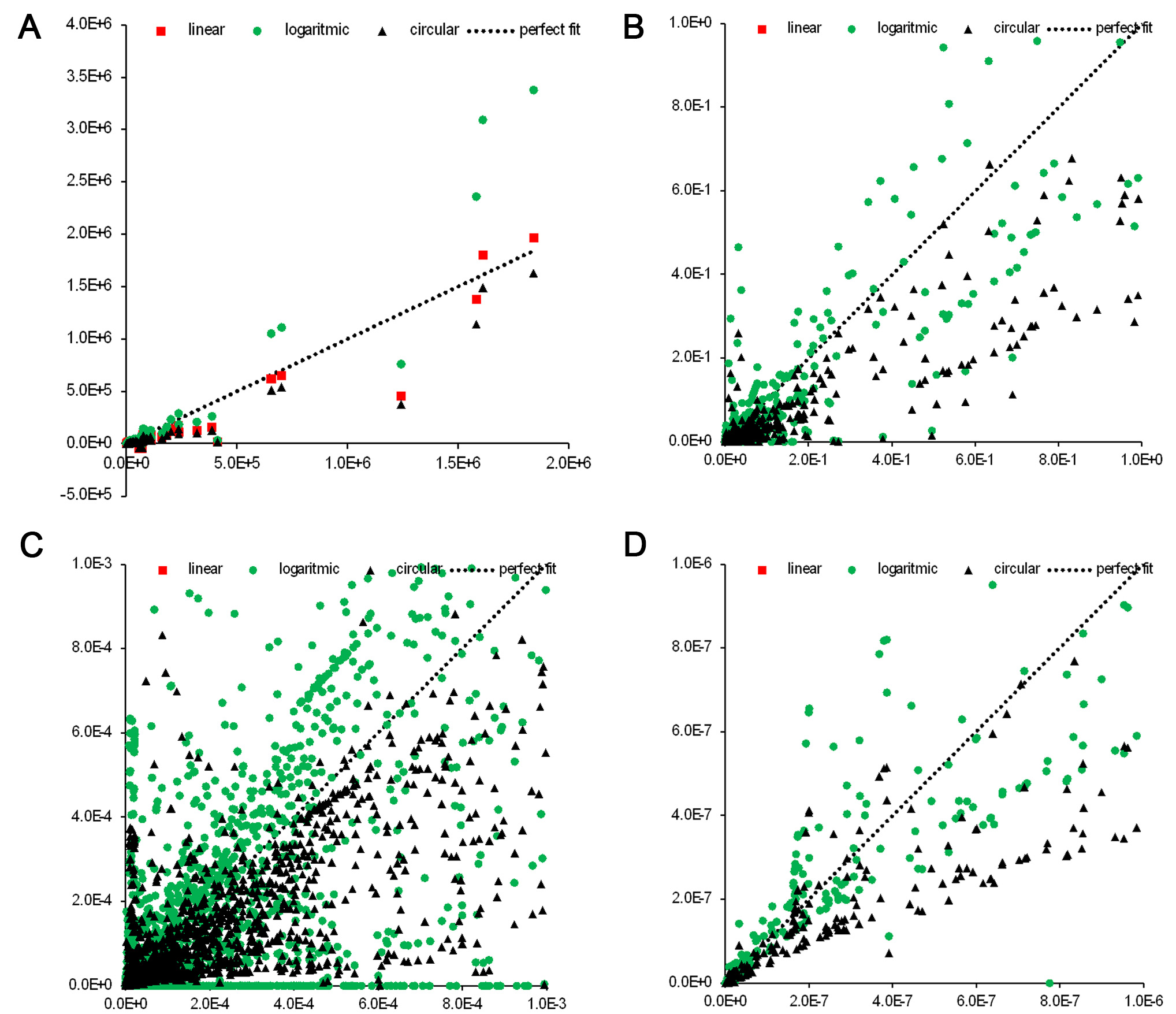
Figure 6. Scatterplots of true (horizontal axis) versus predicted (vertical axis) acidification impacts using three methods. Panel (A) shows the full dataset; panels (B-D) provide zoomed views of regions with smaller values.
Because the true acidification values span approximately 18 orders of magnitude, Figure 6A compresses much of the detail, necessitating the zoomed representations in Figure 6B-D.
Figure 7A shows the distribution of normalized residuals for acidification predictions. From a predictive perspective, the most relevant interval is f
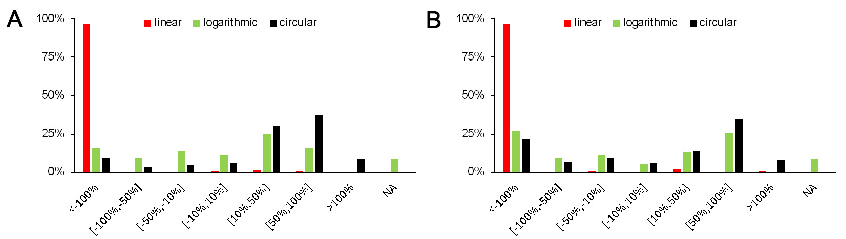
Figure 7. Histograms of normalized residuals for the full sample using three prediction methods: (A) acidification; (B) freshwater ecotoxicity.
Similar patterns are observed for other impact categories. Figure 7B, which presents results for freshwater ecotoxicity, exhibits the same general structure: extremely poor performance for linear regression and comparatively weak, but broadly similar, performance for the logarithmic and circular methods.
DISCUSSION
The CF is a valuable indicator for assessing the climate impact of products, which is particularly relevant given that climate change is widely regarded as a top priority in environmental sustainability. However, CF is not suitable as a proxy for other environmental impact categories. Indeed, the correspondence between CF and other indicators may be even weaker than our already conservative estimates suggest. Many impact categories exhibit substantial regional variability. For example, sulphur oxide emissions have markedly different effects in forested areas compared to marine environments. In addition, these indicators are subject to greater uncertainty, both in terms of parameterization and modeling, particularly for impact categories such as toxicity and resource depletion[6].
A comprehensive environmental assessment therefore requires a multi-indicator approach, in which CF is complemented by dedicated metrics for ozone depletion, toxicity, resource depletion, land use, and other relevant impacts. One example of such an approach is the multidimensional environmental footprint framework adopted by the European Union[21]. More broadly, sustainability policies should account for trade-offs across environmental impact categories and extend beyond the environmental domain to include other dimensions such as economic, social, and governance considerations.
We also reaffirm our conclusion that correlation analysis is not an appropriate analytical tool for assessing whether CF can serve as a proxy for overall environmental impact, or more generally, whether one indicator can reliably predict another. The problem at hand, using CF to predict other impact categories, is more appropriately framed as an analysis of directional relationships, for which directional statistics provides a well-established methodological framework.
Our analysis employs both conventional metrics (r and ρ for overall fit, and e for individual residuals) and newly proposed measures (V and f, respectively). Importantly, none of these metrics is intrinsically dependent on sample size. This contrasts with commonly used statistics such as p-values from hypothesis testing (as in[4,5], and[11]), confidence intervals of regression coefficients (as in[10]), or F-statistics for regression models (as in[9]). These measures tend to indicate increasing significance with larger sample sizes, as standard errors decrease proportionally to
Our argument for moving beyond the conventional regression framework is grounded in its sensitivity to arbitrary choices of units and scaling of product quantities. Directional statistics offers a more consistent approach in this respect. Nevertheless, this method is not without limitations. First, it remains largely unfamiliar to practitioners in the CF and LCA communities. Second, it is not readily implemented in widely used software tools such as Excel. Third, it requires the adoption of heuristic threshold values (e.g., for V) to determine acceptable predictive performance. Despite these limitations, we contend that the theoretical advantages of the directional approach outweigh its practical drawbacks.
CONCLUSION
The results presented in Table 1 may initially suggest a moderate to strong correlation between CF and several other impact categories. For most categories, the Pearson correlation coefficient exceeds 0.90 in both the linear and logarithmic specifications. In contrast, the circular variance yields consistently less optimistic results, with values of 0.02 or higher, well above the rule-of-thumb threshold of 0.001 adopted in this study.
A closer examination of predictive performance, however, reveals substantial limitations across all three methods. We argue that reliance on the conventional residual, yi -
Based on these findings, we conclude that conventional metrics, such as linear or logarithmic Pearson correlation coefficients (r), rank correlation (ρ), and coefficients of determination (R2), can provide a misleading characterization of the relationship between impact categories. In contrast, circular variance offers a more reliable and appropriately cautious indicator of their association.
Overall, our analysis indicates that CF is a poor predictor across all sixteen impact categories considered. Estimating environmental impacts on the basis of CF alone is therefore likely to introduce substantial uncertainty, regardless of whether linear regression, logarithmic regression, or directional statistics are applied. An important advantage of the circular approach is that it avoids overstating predictive performance and thus provides a more realistic assessment of its limitations.
This conclusion remains robust when the analysis is restricted to specific product subgroups. We demonstrate this for infrastructure-related products, which were previously reported in[6] to exhibit comparatively strong correlations.
DECLARATIONS
Acknowledgment
Assistance from Jingcheng Yang for creating several of the figures is appreciated.
Author’s contributions
Made substantial contributions to conception and design of the study and performed data analysis and interpretation, wrote the initial manuscript: Heijungs, R.
Improved the manuscript for better exposition of message: Yang, Y.; Laurent, A.
Checked validity of methods and results, Conceived high-quality graphical presentations: Yang, Y.
Performed data acquisition: Laurent, A.
Availability of data and materials
Excel files with the data to generate the results are available as Supplementary Materials.
AI and AI-assisted tools statement
During the preparation of this manuscript, the AI tool ChatGPT (version GPT-5.3, released 2026-03-03) was used solely for improving its readability and language in the manuscript. The tool did not influence the study design, data collection, analysis, interpretation, or the scientific content of the work. All authors take full responsibility for the accuracy, integrity, and final content of the manuscript.
Financial support and sponsorship
None.
Conflicts of interest
Heijungs, R. and Yang, Y. are Associate Editors of this journal. They were not involved in any steps of editorial processing, notably including reviewers’ selection, manuscript handling and decision making. Laurent, A. declares that there are no conflicts of interest.
Ethical approval and consent to participate
Not applicable.
Consent for publication
Not applicable.
Copyright
© The Author(s) 2026.
Supplementary Materials
REFERENCES
1. ISO. ISO 14067:2018. Greenhouse gases-carbon footprint of products-requirements and guidelines for quantification. International Organization for Standardization, 2018. https://www.iso.org/standard/71206.html (accessed 2026-04-08).
2. Finkbeiner, M. Carbon footprinting - opportunities and threats. Int. J. Life. Cycle. Assess. 2009, 14, 91-4.
3. Yang, Y.; Bae, J.; Kim, J.; Suh, S. Replacing gasoline with corn ethanol results in significant environmental problem-shifting. Environ. Sci. Technol. 2012, 46, 3671-8.
4. Röös, E.; Sundberg, C.; Tidåker, P.; Strid, I.; Hansson, P. Can carbon footprint serve as an indicator of the environmental impact of meat production? Ecol. Indic. 2013, 24, 573-81.
5. Kalbar, P. P.; Birkved, M.; Karmakar, S.; Nygaard, S. E.; Hauschild, M. Can carbon footprint serve as proxy of the environmental burden from urban consumption patterns? Ecol. Indic. 2017, 74, 109-18.
6. Laurent, A.; Olsen, S. I.; Hauschild, M. Z. Limitations of carbon footprint as indicator of environmental sustainability. Environ. Sci. Technol. 2012, 46, 4100-8.
7. Huijbregts, M. A.; Rombouts, L. J.; Hellweg, S.; et al. Is cumulative fossil energy demand a useful indicator for the environmental performance of products? Environ. Sci. Technol. 2006, 40, 641-8.
8. Bösch, M. E.; Hellweg, S.; Huijbregts, M. A. J.; Frischknecht, R. Applying cumulative exergy demand (CExD) indicators to the ecoinvent database. Int. J. Life. Cycle. Assess. 2006, 12, 181-90.
9. Pak, J.; O, N.; Ro, J.; Ri, P.; Ri, T. Correlation analysis of life cycle impact assessment methods and their impact categories in the food sector: representativeness and predictability of impact indicators. Int. J. Life. Cycle. Assess. 2023, 28, 1302-15.
10. Laurenti, R.; Demirer Demir, D.; Finnveden, G. Analyzing the relationship between product waste footprints and environmental damage - a life cycle analysis of 1,400+ products. Sci. Total. Environ. 2023, 859, 160405.
11. Pak, S.; O, N.; Ri, R.; Ro, J.; Ri, P. Applicability of carbon footprint as indicator for environmental performance of food products. Int. J. Environ. Res. 2023, 18, 5.
12. Amer, E. A. A. A.; Meyad, E. M. A.; Meyad, A. M.; Mohsin, A. K. M. The impact of natural resources on environmental degradation: a review of ecological footprint and CO2 emissions as indicators. Front. Environ. Sci. 2024, 12, 1368125.
13. Erhart, S.; Erhart, K. Environmental ranking of European industrial facilities by toxicity and global warming potentials. Sci. Rep. 2023, 13, 1772.
14. Steinmann, Z. J. N.; Schipper, A. M.; Hauck, M.; Giljum, S.; Wernet, G.; Huijbregts, M. A. J. Resource footprints are good proxies of environmental damage. Environ. Sci. Technol. 2017, 51, 6360-6.
15. Heijungs, R.; Dekker, E. Meta-comparisons: how to compare methods for LCA? Int. J. Life. Cycle. Assess. 2022, 27, 993-1015.
18. Cohen, J.; Cohen, P. Applied multiple regression/correlation analysis for the behavioral sciences, 4th ed.; Lawrence Erlbaum Associates, 1983.
19. Neter, J.; Wasserman, W.; Kutner, M. H. Applied linear statistical models: regression, analysis of variance, and experimental designs, 2th ed.; IRWIN, Chicago, 1985. https://archive.org/details/appliedlinearsta00nete/page/n3/mode/2up (accessed 2026-04-14).
20. Heijungs, R. Probability, statistics and life cycle assessment: guidance for dealing with uncertainty and sensitivity. Springer, Cham, 2024.
21. Damiani, M.; Ferrara, N.; Ardente, F. Understanding product environmental footprint and organisation environmental footprint methods. European Union, Luxembourg, 2022. https://publications.jrc.ec.europa.eu/repository/handle/JRC129907 (accessed 2026-04-14).
Cite This Article
How to Cite
Download Citation
Export Citation File:
Type of Import
Tips on Downloading Citation
Citation Manager File Format
Type of Import
Direct Import: When the Direct Import option is selected (the default state), a dialogue box will give you the option to Save or Open the downloaded citation data. Choosing Open will either launch your citation manager or give you a choice of applications with which to use the metadata. The Save option saves the file locally for later use.
Indirect Import: When the Indirect Import option is selected, the metadata is displayed and may be copied and pasted as needed.
About This Article
Copyright

Data & Comments
Data
0


Comments
Comments must be written in English. Spam, offensive content, impersonation, and private information will not be permitted. If any comment is reported and identified as inappropriate content by OAE staff, the comment will be removed without notice. If you have any queries or need any help, please contact us at [email protected].