

Does income growth primarily affect ecological footprint or renewable energy? New evidence from India in the context of the Kuznets hypothesis
 0
0 
Abstract
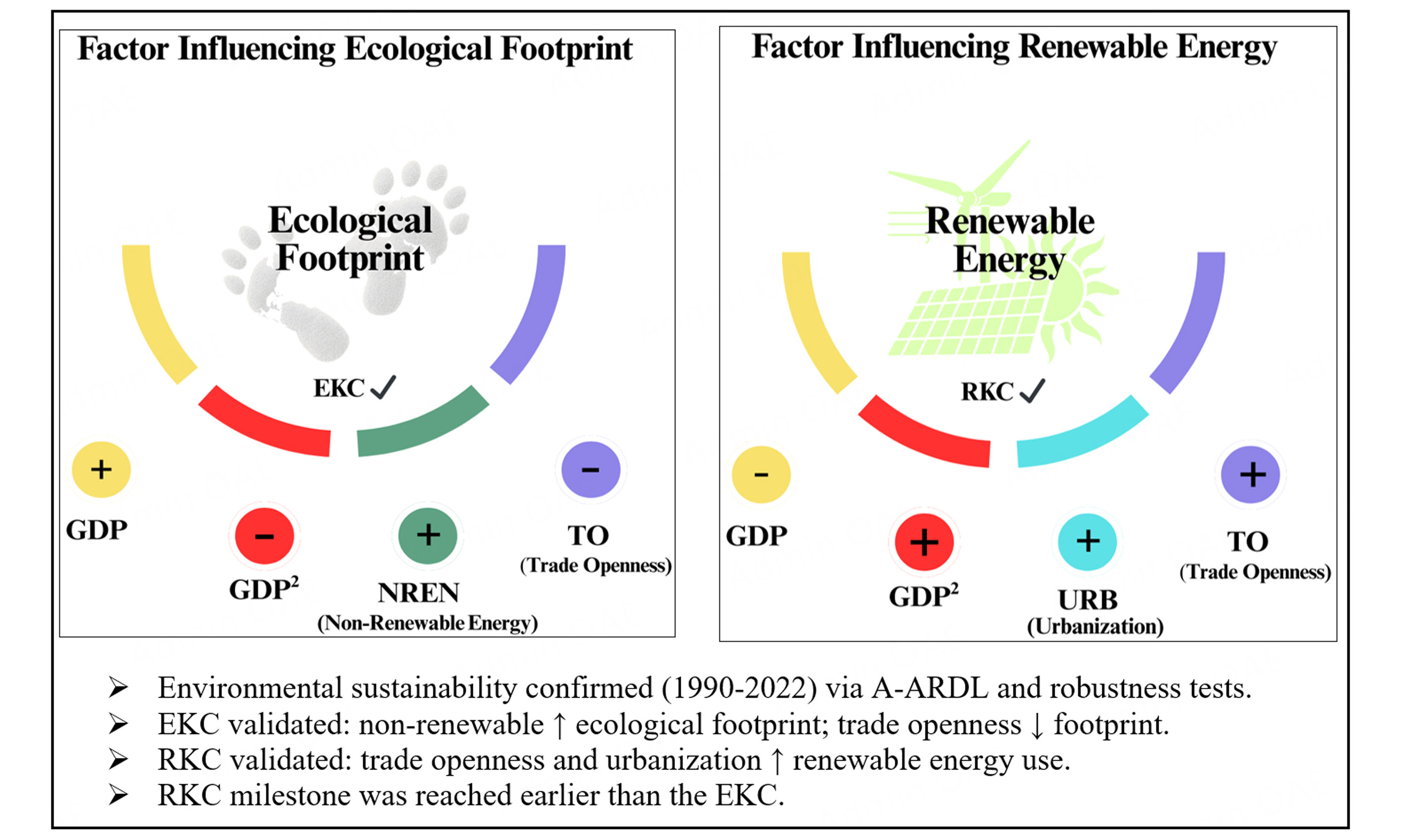
This study investigates the dynamics of environmental sustainability in India, one of the world's major polluters, by examining the validity of the Environmental Kuznets Curve (EKC) and the Renewable Energy Kuznets Curve (RKC) hypotheses for the period 1990-2022. Utilizing an Augmented Autoregressive Distributed Lag (A-ARDL) model, supported by Fully Modified Ordinary Least Square (FMOLS) and Canonical Cointegration Regression (CCR) robustness estimators, the research uniquely determines which of the two Kuznets turning points occurs first. The findings provide strong evidence that the RKC turning point precedes the EKC turning point. This indicates that the shift toward renewable energy adoption begins before the peak of environmental degradation is reached. This result offers critical insights by shedding light on the relationship between economic development and environmental sustainability, suggesting that strategic prioritization of renewable energy can serve as a proactive mechanism to accelerate environmental improvement in a rapidly growing economy such as India.
Keywords
INTRODUCTION
The interplay between economic growth, energy consumption, and environmental sustainability has been a central and often contentious theme in economic discourse. Early perspectives, notably influenced by the "Limits to Growth" report, highlighted the potential unsustainability of growth processes reliant on non-renewable resources[1-3]. This established a foundational tension, with mainstream economists frequently noting the conflict between environmental protection and the energy demands of economic expansion[4-6], while others argued for the potential of technological development and substitution to mitigate negative environmental impacts[7]. The subsequent introduction of the sustainable development concept provided a more nuanced framework for analyzing this complex relationship.
A seminal contribution within this framework was the Environmental Kuznets Curve (EKC) hypothesis, first framed by Panayotou based on the foundational work of Grossman and Krueger[8,9]. The EKC posits an inverted U-shaped relationship, suggesting that environmental pollution initially increases with economic growth due to the scale effect, but eventually declines as economies undergo structural transformations and adopt cleaner technologies, driven by the structural and technological effects[9].
More recently, the theoretical landscape has been enriched by the introduction of the Renewable Energy Kuznets Curve (RKC) hypothesis, proposed by Yao et al.[10] as a complementary perspective. The RKC describes a U-shaped relationship between per capita income and renewable energy consumption (REN). According to this hypothesis, REN initially decreases as developing economies prioritize inexpensive fossil fuels to power their growth. However, after reaching a certain income threshold - supported by strong financing infrastructure and welfare gains[3,11] - rising environmental awareness and technological progress lead to an increase in renewable energy adoption. A critical theoretical proposition is that the income level corresponding to the RKC's turning point should be lower than that of the EKC's peak. This suggests that a successful transition toward renewable energy is a prerequisite for achieving long-term environmental improvement, causing the RKC to "turn" before the EKC[10].
Determining which of the turning points occurs first is not merely an academic exercise; it holds profound significance for national policy design. This presents a crucial window of opportunity for policymakers to implement targeted policies, such as renewable infrastructure investments and green incentives, to "flatten" the EKC and accelerate the path to sustainability. This question is especially pertinent for a country such as India, the world's third-largest polluter, which is simultaneously navigating the pressures of rapid economic development.
Despite a vast body of literature on the validity of the EKC in the Indian context, studies investigating the RKC hypothesis - and critically, its temporal relationship with the EKC - are non-existent. This study aims to fill this significant gap in the literature by empirically investigating which turning point occurs first in the Indian economy. To achieve this, we develop two distinct models to test the EKC and RKC hypotheses using data from 1990 to 2022. By calculating and comparing the turning points of both curves through contemporary and robust econometric methods, this research provides the first empirical evidence on this matter for India. The findings are intended to offer novel and actionable insights for India's energy and environmental policy, providing strategic guidance on prioritizing developmental goals while fostering a sustainable future. The remainder of this study is organized as follows. In the Section "LITERATURE REVIEW", the literature on EKC and RKC hypotheses is discussed in detail, and the relationships of other variables used in the models are examined in depth. In the Section "DATA, MODEL CONSTRUCTION AND METHODOLOGY", the data set and models used in the study are introduced and the empirical methodology is given. In the Section "EMPIRICAL FINDINGS", the study findings are summarized. In the Section "DISCUSSION", the results obtained from the study are evaluated. In the Sections "CONCLUSION" and "DECLARATIONS", the findings are discussed and policy recommendations are presented.
LITERATURE REVIEW
In this section, the theoretical foundations of the study - the Environmental Kuznets Curve (EKC) and Renewable Energy Kuznets Curve (RKC) hypotheses - are discussed in depth within the framework of empirical findings from the relevant literature. First, we focus on EKC-based studies examining the effects of trade openness (TO) and non-renewable energy consumption (NREN) on the ecological footprint. Second, we review literature on the more recent RKC hypothesis, which explores the relationships among variables such as urbanization, TO, and REN. Finally, the interaction between these two hypotheses is discussed, and the research gap addressed by the present study is identified.
Environmental Kuznets curve (EKC) hypothesis and its determinants
Many studies have been conducted on EKC over the last thirty years. They have related per capita income with pollution variables such as CO2, ecological footprint (EF), and carbon footprint[10,12]. It can be said that the studies on EKC generally address four main issues. These can be summarized as income, financial development, technological development, and environmental regulations[12,13]. However, most recently, the Paris Climate Agreement, toward the implementation of environmental policies among countries, has brought growth processes based on renewable energy sources to the fore. Renewable energy is a key component linked to economic growth, social concerns, and environmental sustainability[13]. Despite this finding, the share of renewable energy in total energy consumption in the world is still around 10%, although it varies from country to country[14]. In recent years, more comprehensive variables such as the EF have been included in the analysis as an environmental indicator. Research on the determinants of the ecological footprint has focused particularly on the effects of variables such as TO and NREN.
The role of TO as a determinant presents contradictory findings in the literature. Some studies argue that trade exacerbates environmental degradation. For instance, Adebayo et al.[15], in their analysis of MINT (Mexico, Indonesia, Nigeria, Turkey) countries, found that TO positively affects the ecological footprint in the short and medium term in Mexico and Indonesia, and across all terms in Turkey and Nigeria. Similarly, Abdullahi et al.[16] for the Economic Community of West African States (ECOWAS) countries, Zhou et al.[17] for Belt and Road Initiative (BRI) countries, Zahid et al.[18] for BRICS countries, and Van Hek et al.[19] for 10 Newly Industrialized Countries (NICs) concluded that international trade increases the EF. In contrast, another group suggests that trade can improve environmental quality by facilitating the diffusion of cleaner technologies. Alqaralleh[20] states that a positive TO shock reduces environmental degradation in ASEAN countries, while Dam et al.[21] for E7 countries and Cutcu et al.[22] for the USA have provided evidence that international trade reduces the EF in the long run. Gao et al.[23] state that the EKC is not merely an empirical phenomenon but can be shaped by policy objectives. For example, Cao et al.[24], in their study on China's minority regions, propose a policy of "flattening the EKC" through industrial and green technological innovation to achieve sustainable development goals. Green finance also plays a critical role in this transformation. Indeed, Zhang et al.[25] empirically demonstrate that China's Pilot Zone for Green Finance (PZGFRI) policy has significantly increased green innovation through capital and research and development (R&D) support. This demonstrates that targeted financial policies can accelerate environmental improvement by triggering technological innovation.
In addition to TO, another significant determinant of the ecological footprint is NREN. One of the most important sub-components of the ecological footprint is the carbon footprint, and its primary source is non-renewable energy. Therefore, there is a strong consensus in the literature that NREN increases the EF. In a study specific to India, Roy[26] analyzed the 1990-2016 period using the Autoregressive Distributed Lag (ARDL) technique and found that NREN has a positive long-run effect on the EF. This finding is supported by studies on other countries and regions. Adekoya et al.[27] showed that NREN increases the EF in both 14 net oil-exporting and 14 net oil-importing countries. Idroes et al.[28] for Indonesia, Destek and Sinha[29] for 24 OECD countries, Dogan et al.[30] for South Asian countries, Kongkuah[31] for BRI countries, and Pata[32] for the USA have all reported the same effect.
Renewable energy Kuznets curve (RKC) hypothesis and its determinants
The RKC hypothesis, developed by Yao et al.[10] as an alternative to the EKC hypothesis, proposes a U-shaped relationship between income growth and REN. This hypothesis, contrary to the EKC, posits that REN decreases in the initial stages of economic development but begins to increase after a certain income threshold is passed. Many studies in the literature have focused on the mitigating effect of REN on CO2 emissions, but have not made any inferences about how the widespread adoption of REN would affect the turning point or the economic rationale behind it[10]. While the economy is under the "scale effect", per capita GDP increases, but REN decreases because the energy required during the rapid growth process is primarily sourced from fossil fuels.
As the RKC hypothesis is relatively new, the literature remains in its developmental stages.
The literature has also examined the effects of variables such as urbanization and TO on REN. Urbanization, defined as the migration of rural populations to cities, creates problems related to access to clean air and water, stemming from NREN[25,33,34]. The impact of urbanization on renewable energy, however, is ambiguous. Some studies have found a positive relationship. For instance, Khan et al.[35] showed that in 48 BRI countries, urbanization reduces carbon emissions and that REN also has a reducing effect on carbon emissions. Chen[36], for the Chinese economy, and Kusiyah et al.[37], for 23 industrialized countries, identified a positive interaction between urbanization and REN. On the other hand, some studies have reported a negative relationship. Yin and Qamruzzaman[38] for Bay of Bengal Initiative for Multi-Sectoral Technical and Economic Cooperation (BIMSTEC) countries and Simeon et al.[39] for Emerging Seven (E7) countries showed that urbanization adversely affects renewable energy use. Raihan[40], however, found that for Bangladesh, urbanization increases energy consumption that leads to low carbon emissions.
The effects of TO on REN also feature prominently in the literature. A comprehensive analysis by Wang and Zang[42], covering 186 countries, revealed that free trade positively affects REN in high and upper-middle-income countries but negatively in low-middle-income countries, while Zeren and Akkuş[43] found that increases in energy consumption reduce TO in Bloomberg's Top Emerging Countries. Han et al.[44] concluded that in the Chinese economy, TO partially increases REN but invariably increases NREN. Similarly, Khan et al.[45] found that TO facilitates the transition to renewable energy in developed countries but has a negative impact in developing countries. In contrast, other studies focused on specific country groups have generally identified a positive relationship. Alam and Murad[46], for OECD countries, Murshed[47], for South Asian countries, Jóźwik et al.[48], for the top 15 countries in REN, and Zhongwei and Liu[49], for the Group of Twenty (G20), all concluded that TO increases REN.
Literature gap
India is the third-largest polluting country, after China and the USA. Despite numerous national and international measures, it has recently become the world leader in the rate of increase in environmental pollution. Meanwhile, India is among the fastest-growing economies. The natural consequence of these two factors is increased energy consumption, which has been the subject of many studies. There exists a substantial body of literature on the validity of the EKC hypothesis. However, the RKC hypothesis, which argues the opposite of the inverted-U hypothesis put forward by the EKC hypothesis, is quite new. Moreover, there is no study on India where the EKC and RKC hypotheses are used together and addressed within the framework of robustness testing. This study is primarily motivated by the question of which occurs first in India as income rises: environmental degradation or the increase in REN. The answer to this question, which is thought to make a significant contribution to the literature, addresses both the validity of the EKC and RKC hypotheses and the priority of the environmental consequences of income. Moreover, the study provides a theoretical contribution to the relevant literature by using advanced time series techniques and robustness tests, and also performs an empirical comparison. It is evaluated that the study will contribute to the relevant field and fill the gap in the literature within the framework of the factors in question.
DATA, MODEL CONSTRUCTION AND METHODOLOGY
In this section, the dataset is first introduced, followed by its basic features. The next section presents information about the established models, and the methodology used in the study is then described.
Data
Two different models are established in the study. Information on the variables used in the models is given in Table 1, providing data for the 1990-2022 sample period for India.
Information on the variables used
| Symbol | Category | Variables | Description and measurement | Source |
| EF | Dependent variable | Ecological Footprint | Ecological Footprint vs Biocapacity (gha per person) | Global Footprint Network (2025) |
| REN | Dependent variable | Renewable energy | Quadrillion Btu | EIA (2025) |
| GDP | Independent variable | Income | GDP per capita (constant 2015 USD) | World Bank (2025) |
| GDP2 | Independent variable | Income Squared | GDP per capita (constant 2015 USD) | World Bank (2025) |
| NREN | Independent variable | Fossil energy consumption | Quadrillion Btu | EIA (2025) |
| TO | Independent variable | Trade openness | The ratio of total exports and imports to GDP | World Bank (2025) |
| URB | Independent variable | Urbanization | Urbanization (% of total population) | World Bank (2025) |
Table 1 provides information on all the data to be used in two different models. In this context, the EF and REN variables will be used as dependent variables. These variables were obtained from the Global Footprint Network[50] and the US Energy Information Administration (EIA)[51], respectively. To utilize the quadratic form, the GDP and GDP2 variables will be used in the empirical models. These variables were obtained from the World Bank[52]. The variables designated as TO and urbanization (URB) were also obtained from the World Bank and included in the model as ratio variables. Descriptive statistics for the data are provided in Table 2.
Descriptive statistics
| Stat. | EF | REN | GDP | GDP2 | NREN | TO | URB |
| Mean | -0.16 | 0.28 | 6.93 | 48.17 | 2.74 | 3.52 | 3.39 |
| Median | -0.21 | 0.28 | 6.91 | 47.83 | 2.70 | 3.69 | 3.39 |
| Max. | 0.08 | 1.32 | 7.64 | 58.42 | 3.24 | 4.02 | 3.58 |
| Min. | -0.38 | -0.34 | 6.28 | 39.39 | 2.25 | 2.74 | 3.24 |
| Std. Dev. | 0.16 | 0.52 | 0.44 | 6.15 | 0.32 | 0.39 | 0.10 |
| Skew. | 0.08 | 0.45 | 0.10 | 0.16 | 0.07 | -0.44 | 0.21 |
| Kurt. | 1.48 | 1.91 | 1.68 | 1.69 | 1.59 | 1.83 | 1.80 |
| J-B | 3.22 (0.20) | 2.75 (0.25) | 2.46 (0.29) | 2.50 (0.29) | 2.76 (0.25) | 2.97 (0.23) | 2.23 (0.33) |
Descriptive statistics of EF, REN, GDP, GDP2, NREN, TO and URB variables for India are reported in Table 2. It was observed that all variables for India exhibited normal distribution at 1% significance level in the period 1990-2022.
Model construction
This section contains information about the model established. In the study, two models are established to measure the EKC and RKC hypotheses. The model for the EKC hypothesis was established in (1), and the model for the RKC hypothesis in (2). In model (1), NREN and TO variables were used in addition to EF, GDP, and GDP2. Although non-renewable energy use in the Indian economy has recently declined, it remains high. In this context, NREN is included in model (1) to determine its impact on EF, an indicator of environmental degradation. Furthermore, in the globalization era, TO has increased globally. This trend is lower in India. Understanding the impact of TO on environmental degradation is considered important for Indian economic policies. In this context, TO was added to model (1). In model (2), the focus is on the relationship between REN and GDP and GDP2. Because of the high correlation between NREN and REN, the NREN variable was not included in the model. Rapidly increasing urbanization in India can also lead to environmental consequences. In this context, the relationship between renewable energy and urbanization can become important. Therefore, the TO variable was added to model (2) to form an empirical model. In both models, the natural logarithm of the variables was taken. Mishra et al.[53] and Mishra et al.[54] suggested that consistent and reliable findings were achieved by taking the natural logarithmic transformations of the variables. Therefore, it is stated that the models lead to more consistent and robust results. The relevant models are expressed as
where t indicates the sample period of 1990-2022. In both models, the constant terms are indicated as β10 and β20, respectively. In model (1), where the EKC hypothesis will be tested, β11, β12, β13, and β14 indicate the elasticity coefficients of GDP, GDP2, NREN, and TO, respectively. In model (2), where the RKC hypothesis will be tested, β21, β22, β23, and β24 indicate the elasticity coefficients of GDP, GDP2, TO, and URB, respectively. Finally, ε1t and ε2t symbolize the error term of models (1) and (2), respectively. Figure 1 shows the graphs of the variables used in the models.
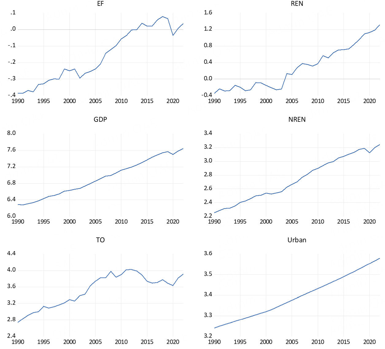
Figure 1. Time path graphs of variables.
Methodology
This section of the study focuses on the econometric method used in the analysis. For this purpose, first, the Augmented Dickey Fuller (ADF) and Phillips-Perron (PP) unit root tests and the Fourier ADF unit root test are introduced, and then the A-ARDL cointegration technique is discussed. In the following section, Fully Modified Ordinary Least Square (FMOLS), Dynamic Ordinary Least Square (DOLS), and Canonical Cointegration Regression (CCR) methods that provide long-term cointegration coefficients are explained. Finally, the Fourier Bootstrap Toda-Yamamoto (FBTY) Causality technique is presented to investigate the short-term causality interaction between variables. A summary of the methodology used is given in Figure 2.
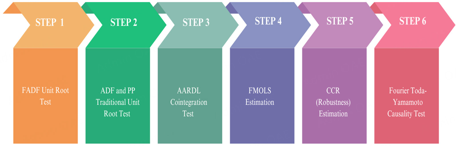
Figure 2. Econometric framework.
Unit root tests
In the analysis, the ADF unit root test and PP unit root test are used for the unit root research of the variables examined[55,56]. The PP unit root test has a significant advantage over the ADF unit root test. The PP test provides robust results in the cases of serial correlation in the considered series, time-sensitive heteroscedasticity, and time-dependent regime change in the sample period[57]. It is considered important to account for structural breaks in the investigation of the unit root process. In this context, Christopoulos and León-Ledesma[58] developed a new Fourier-based unit root test that simultaneously considers the nonlinear fitting process and structural breaks. The new Fourier-based unit root test includes structural breaks by considering a trigonometric function that allows smooth temporal mean changes, in addition to the linear fitting process modeled by smooth transition functions. The main advantage of this test is that it does not consider the factors causing the structural break as external[58].
yt, a stochastic process, is defined as follows:
where δ(t) is the time-varying deterministic component and υt ~ N(0, σ). Christopolous and
where, k is the frequency number of the Fourier Function, t is the trend term, T is the sample size and
In this case, the Fourier-based ADF unit root test for the yt series, considered a stochastic process, is performed using the following steps. In the first step, the optimal frequency number is determined to minimize the error terms obtained from Equation (6) estimated with Ordinary Least Square (OLS).
After estimating this Equation, the error term is obtained as
In the second stage, the Fourier-ADF test is applied to the error term obtained in the first stage. For this, Equation (8) is estimated and the relevant hypothesis tests are established.
where μt is the noisy error term. The null hypothesis (H0) for the unit root test is H0:β1 = 0 and the alternative hypothesis (HA) is HA:β1 ≠ 0. If the H0 testing the existence of a unit root is rejected using the critical values calculated by Christopolous and Leon-Ledesma[58], the third stage is passed. In the third stage, if the H0 expressing the existence of a unit root is rejected in the second stage, the coefficients of the trigonometric function in Equation (8) are tested. For this purpose, the H0 to be established is H0:δ1 = δ2 = 0 and the HA is
A-ARDL cointegration
McNown et al.[63] and Pesaran et al.[64] developed the Augmented Autoregressive Distributed Lag (A-ARDL) bounds test approach based on the ARDL bounds test model, which was introduced to the literature by Pesaran et al.[64] and used by many researchers in the last twenty years. The A-ARDL model, similarly to the ARDL model, yields successful results in small samples and offers the opportunity to obtain short- and long-term dynamics. Another advantage of the ARDL model over traditional cointegration tests is that it allows the independent variables to be I(0) or I(1), provided that the dependent variable is I(1). The superiority of the A-ARDL technique over the ARDL technique is that it includes the condition that the dependent variable is also I(0)[63]. The A-ARDL model developed by McNown et al.[63] stated that the FOV (test expressing the coefficients of the first lags of the dependent variable and the independent variables) and tDV (first lag of the dependent variable) tests presented for cointegration in the ARDL model developed by Pesaran et al.[64] may give incorrect cointegration results, and therefore, researchers using the ARDL model may suggest incorrect economic policies. Accordingly, two types of degenerate situations may occur when conducting cointegration research in the ARDL model by Pesaran et al.[64]. The first of these is the situation where the test statistic of the lagged value of the dependent variable is insignificant, and the second is the situation where the lagged values of the independent variables are insignificant as a whole. It is argued that in the event of degenerate situations, the error term gap between the dependent and independent variables will not be closed, and therefore, cointegration inference cannot be made[65].
The significant result of the FOV test indicates that the lagged levels of the dependent variable and the independent variables are integrated. However, the significant result of the FOV test may indicate that only the lagged state of the dependent variable is significant or only the lagged states of the independent variables are significant together. Accordingly, if only tDV is significant, the ARDL equation becomes the ADF regression equation, and in this case, the dependent variable becomes I(0).
McNown et al.[63] proposed an additional robustness test based on the significance of the lagged independent variables as a whole (FIV) instead of the assumption that the dependent variable is I(1). The main advantage of the additional test is that it relaxes the condition that the dependent variable is I(1) to exclude the degenerate case.
In order to make a cointegration inference in the A-ARDL model, the FOV and tDV tests suggested by
Mcnown et al.[63] proposed a critical value calculation method based on the bootstrap process for the FIV test, which they proposed to test the joint significance of the lagged states of the independent variables. However, since this method was problematic in terms of application, Sam et al.[65] created the critical value table by proving the basic theorems and making the necessary calculations.
The A-ARDL model can be expressed by
The H0 of cointegration is tested through
(i) FOV test for lagged levels of all variables: H0:byy = byx,x = 0 and HA:byy = byx,x ≠ 0.
(ii) tDV test for the lagged level of the dependent variable: H0:byy = 0 and HA:byy ≠ 0.
(iii) FIV test for lagged levels of independent variables: H0:byx,x = 0 and HA:byx,x ≠ 0.
Accordingly, if FOV and tDV are significant but FIV is insignificant, there is a degeneration based on the lagged levels of the independent variables. The statistical insignificance of the lagged levels of the independent variables transforms the ARDL equation into the DF equation. In this case, the significance of the FOV test is due to the tDV test. Therefore, in this case, the dependent variable is I(0). Despite this, there is no cointegration. On the other hand, if FOV and FIV are significant but tDV is insignificant, there is a degeneration based on the lagged levels of the dependent variable. Therefore, the linear combinations of the variables used in the model do not move together in the long run. The cointegration interaction is obtained only when all three tests mentioned above reject H0 at the same time.
FMOLS and CCR estimators
The techniques commonly used in the literature to test the robustness of the estimation results obtained from the A-ARDL model are: FMOLS and CCR. Long-term coefficients can be obtained using these cointegration techniques.
FMOLS, developed by Phillips and Hansen[66], offers a semi-parametric correction technique to eliminate the problems arising from the endogeneity problem between the variables examined in the model. Thus, the FMOLS estimator is obtained by eliminating the deviation and endogeneity problems in the OLS estimator. The FMOLS estimator eliminates the autocorrelation and endogeneity problems that occur in the OLS estimator, allowing more consistent results to be obtained in small samples.
Park[67] proposed the CCR model for the coefficient estimates of the variables included in the cointegration model. CCR is closely related to FMOLS and, unlike FMOLS, it simultaneously corrects the variables used in the model. However, FMOLS performs the correction process in series, one by one. Using this method, Park demonstrated that efficient and unbiased estimators such as FMOLS can be achieved[67].
Fourier bootstrap Toda-Yamamoto causality
Nazlioglu et al.[68] proposed a new causality test formed by modeling gradual structural breaks with the Fourier function. This test is obtained by expanding the Toda-Yamamoto test with the trigonometric function. Enders and Jones[69] stated that if structural breaks are neglected, the established Vector AutoRegressive (VAR) model will be underdefined and therefore incorrect hypothesis test results may occur. Based on this, Nazlioglu et al.[68] added the Fourier function to the Toda-Yamamoto causality test including soft structural breaks. Accordingly, the FBTY causality test can be established as
where the constant term ϕ(t) shows the possible structural changes that occur over time, and et is the white noise error term. To show the structural changes in an unknown date, in an unknown number, and in an unknown form as a gradual process, the single-frequency Fourier Toda-Yamamoto approach can be modeled as follows:
where k is the optimal frequency number, t is the time trend, T is the number of observations, λ1 and λ2 are the parameters measuring the displacement and number of frequencies. Here, the H0 that there is no causality between the variables is H0:δ1 = δ2 = … = δp = 0. The optimal frequency number and lag length are determined by the Akaike information criterion.
EMPIRICAL FINDINGS
This section presents empirical test results for the validity of the EKC and RKC hypotheses specified with models (1) and (2). First, the FADF unit root test findings are reported. The results of the constant and constant-and-trend model tests for all variables used in both models are given in Table 3.
Fourier ADF test findings
| Model with a constant | Freq. | FADF stat. | F(k) | Min. RSS | Crit. val. (10%; 5%; 1%) | |
| FADF test | F test | |||||
| EF | 1 | -2.00 (0) | 42.89 | 0.21 | -3.52; -3.85; -4.43 | 4.13; 4.93; 6.73 |
| REN | 1 | -0.92 (0) | 29.11 | 2.91 | ||
| GDP | 1 | -0.67 (1) | 28.46 | 2.16 | ||
| GDP2 | 1 | -0.60 (1) | 28.45 | 418.42 | ||
| NREN | 1 | -1.19 (0) | 32.00 | 1.03 | ||
| TO | 1 | -1.40 (0) | 52.30 | 1.09 | ||
| URB | 1 | 0.19 (1) | 25.03 | 0.13 | ||
| Model with a constant and a linear trend | Freq. | FADF stat. | F(k) | Min. RSS | Crit. val. (10%; 5%; 1%) | |
| FADF test | F test | |||||
| EF | 2x | -3.79 (0) | 14.59 | 0.030 | -4.15; -4.46; -5.11 | 4.16; 4.97; 6.87 |
| REN | 1 | -3.23 (0) | 20.79 | 0.27 | ||
| GDP | 1 | -3.88 (0) | 18.73 | 0.02 | ||
| GDP2 | 1 | -4.26 (1) | 29.62 | 3.84 | ||
| NREN | 1 | -3.19 (0) | 16.65 | 0.02 | ||
| TO | 1 | -2.64 (0) | 54.38 | 0.27 | ||
| URB | 1 | -0.38 (0) | 125.77 | 0.00 | ||
According to the fixed model results in Table 3, it was observed that the FADF test statistics of all variables were smaller than the critical values calculated by Christopoulos and León-Ledesma[58]. This situation shows that the H0 showing the existence of a unit root could not be rejected. Therefore, the FADF unit root results according to the fixed model showed that all variables had a unit root at the level. According to the fixed and trend model results, it was seen that the EF variable was stationary at a significance level of 10%. The GDP2 variable was stationary at a significance level of 5%. It was concluded that the other variables had a unit root process at the level in the fixed and trend model. To report the obtained results, it should be examined whether the F test was significant or not. It was observed that all F test statistics obtained in the fixed and fixed and trend models of all variables were larger than the critical values presented by
As a result of FADF findings, it was found that EF and GDP2 variables were stationary or unit rooted in fixed and fixed and trend models, while other variables were unit rooted at the level. ADF and PP unit root tests were used to determine the level of stationarity. Table 4 shows the results of traditional unit root tests.
ADF and PP unit root test results
| Variables | ADF | PP | |||
| Level | First difference | Level | First difference | ||
| Constant | EF | -0.81 (0.80) | -5.92*** (0.00) | -0.78 (0.81) | -5.94*** (0.00) |
| REN | 0.74 (0.99) | -5.73*** (0.00) | 1.81 (0.99) | -5.75*** (0.00) | |
| GDP | 0.60 (0.99) | -5.70*** (0.00) | 0.75 (0.99) | -6.17*** (0.00) | |
| GDP2 | 0.93 (0.99) | -5.60*** (0.00) | 1.26 (0.99) | -5.91*** (0.00) | |
| NREN | -0.08 (0.94) | -5.75*** (0.00) | -0.08 (0.94) | -5.75*** (0.00) | |
| TO | -1.91 (0.32) | -4.83*** (0.00) | -1.89 (0.33) | -4.83*** (0.00) | |
| URB | -1.10 (0.70) | -5.96*** (0.00) | -1.14 (0.69) | -5.96*** (0.00) | |
| Constant and trend | EF | -1.94 (0.61) | -5.86*** (0.00) | -1.94 (0.61) | -5.89*** (0.00) |
| REN | -1.87 (0.64) | -6.12*** (0.00) | -1.69 (0.73) | -9.53*** (0.00) | |
| GDP | -3.26* (0.09) | -5.60*** (0.00) | -3.29* (0.08) | -6.05*** (0.00) | |
| GDP2 | -3.07 (0.13) | -5.59*** (0.00) | -3.08 (0.13) | -6.15*** (0.00) | |
| NREN | -2.00 (0.58) | -5.66*** (0.00) | -2.05 (0.55) | -5.66*** (0.00) | |
| TO | -1.32 (0.86) | -4.95*** (0.00) | -1.40 (0.84) | -4.96*** (0.00) | |
| URB | -1.44 (0.83) | -6.01*** (0.00) | -1.47 (0.82) | -6.02*** (0.00) | |
According to ADF and PP findings in the fixed and trend model in Table 4, it was seen that the GDP variable was I(0) at a 10% significance level. All other variables were stationary in the first difference. In other words, all other variables exhibited the I(1) feature. Therefore, it was understood that the variables were not I(2). As a result of FADF, ADF, and PP unit root tests, it was seen that all variables were I(1) or
A-ARDL cointegration test results
| Model-1 | k | Test statistics | I(1) critical values | |||
| 1% | 5% | 10% | ||||
| A-ARDL(1,1,1,1,1) | 4 | FOV 4.98* | 7.172 | 5.304 | 4.512 | |
| tDV -4.33* | -4.96 | -4.36 | -4.04 | |||
| FIV 3.79* | 6.69 | 4.61 | 3.74 | |||
| Diagnostic tests | Test statistics | Probability values | ||||
| Breusch-Godfrey | 1.96 | 0.18 | ||||
| White | 31.59 | 0.44 | ||||
| Ramsey RESET | 2.57 | 0.13 | ||||
| Jarque-Bera | 0.44 | 0.80 | ||||
| CUSUM | Stable | |||||
| CUSUMQ | Stable | |||||
| Model-2 | k | Test statistics | I(1) critical values | |||
| 1% | 5% | 10% | ||||
| A-ARDL(1,2,1,1,1) | 4 | FOV 4.82869* | 7.17 | 5.30 | 4.51 | |
| tDV -4.65815** | -4.96 | -4.36 | -4.04 | |||
| FIV 3.86720* | 6.69 | 4.61 | 3.74 | |||
| Diagnostic tests | Test statistics | Probability values | ||||
| Breusch-Godfrey | 2.00 | 0.16 | ||||
| White | 33.19 | 0.36 | ||||
| Ramsey RESET | 1.24 | 0.28 | ||||
| Jarque-Bera | 0.14 | 0.93 | ||||
| CUSUM | Stable | |||||
| CUSUMQ | Stable | |||||
Table 5 shows the fixed and trend A-ARDL results of the two models used in the study. As seen in the table, there are three different test statistics in this method. The H0 in all relevant tests indicates that there is no cointegration. According to the A-ARDL method, the H0 of the three test statistics must be rejected to reach the conclusion that there is a cointegration interaction. The test statistics in question are FOV, tDV, and FIV. The relevant test statistics are compared with the critical values produced by Narayan[71], Pesaran et al.[64], and Sam et al.[65], respectively. If there is a test statistic above the upper limit value of I(1), then the existence of cointegration is reached. According to the results of Model-1 and Model-2 in Table 5, it has been determined that all three test statistics are greater than the relevant critical values. This situation has revealed the existence of a cointegration interaction in both models according to the A-ARDL method. In addition to these results, the diagnostic tests of the models need to be examined. According to these tests, there is no autocorrelation problem, constant variance is valid, there is no modeling error, and the validity of the normal distribution has been achieved. Therefore, it has been understood that the A-ARDL findings can be used.
After proving the existence of the long-term relationship, estimator tests are used to determine the long-term elasticity coefficients. In this context, the FMOLS[66] results are given first. Then, the CCR[56] estimator is used as a robustness test. Table 6 shows the Model-1 results in which the EKC hypothesis is tested.
Model-1 FMOLS and CCR (robustness) results
| Variables | FMOLS (dependent variable:EF) | |||
| Coeff. | Std. error | t-statistic | P-value | |
| GDP | 2.11*** | 0.54 | 3.89 | 0.00 |
| GDP2 | -0.14*** | 0.04 | -3.91 | 0.00 |
| NREN | 1.08*** | 0.15 | 7.30 | 0.00 |
| TO | -0.05* | 0.03 | -1.75 | 0.09 |
| C | -10.34*** | 1.98 | -5.21 | 0.00 |
| T | -0.02*** | 0.00 | -5.12 | 0.00 |
| Variables | CCR (robustness) | |||
| Coeff. | Std. error | t-statistic | P-value | |
| GDP | 2.17*** | 0.64 | 3.40 | 0.00 |
| GDP2 | -0.14*** | 0.04 | -3.37 | 0.00 |
| NREN | 1.09*** | 0.15 | 7.26 | 0.00 |
| TO | -0.05 | 0.03 | -1.54 | 0.13 |
| C | -10.61*** | 2.32 | -4.58 | 0.00 |
| T | -0.02*** | 0.00 | -5.41 | 0.00 |
Table 6 shows the results of FMOLS and CCR (robustness) estimators. Accordingly, a 1% increase in GDP, GDP2, NREN, and TO causes a 2.11% increase, a 0.14% decrease, a 1.08% increase, and a 0.05% decrease in EF, respectively. While the effects in question are valid at a 10% significance level in TO, they are valid at a 1% significance level in other variables. On the other hand, it is meaningful to use the fixed and trend model results in FMOLS estimation. As a matter of fact, it was obtained that the C and T terms were statistically significant. As a result, the Model-1 results testing the EKC model revealed that the EKC hypothesis was valid. The coefficient that constitutes the main focus of the study is to obtain the degree of the turning point calculated as
The CCR estimator in Table 6 is used as a robustness test. According to the CCR results, a 1% increase in GDP, GDP2, NREN, and TO causes a 2.17% increase, a 0.14% decrease, a 1.09% increase, and a 0.05% decrease in EF, respectively. The effects in question are also statistically insignificant for the TO variable. The other variables are significant at the 1% significance level. On the other hand, similar to the FMOLS results, the C and Trend variables are also significant. Similar to the FMOLS results, the CCR estimator has also strengthened the results and proven the existence of the EKC hypothesis. The turning point is obtained as
Table 7 shows the results of Model-2 established to test the RKC hypothesis.
Model-2 FMOLS and CCR (robustness) results
| Variables | FMOLS (dependent variable:REN) | |||
| Coeff. | Std. ERROR | t-statistic | P-value | |
| GDP | -14.15*** | 2.66 | -5.31 | 0.00 |
| GDP2 | 1.02*** | 0.20 | 5.13 | 0.00 |
| TO | 0.46*** | 0.13 | 3.46 | 0.00 |
| URB | 3.42 | 2.05 | 1.67 | 0.11 |
| C | 36.01*** | 11.85 | 3.04 | 0.00 |
| T | -0.12* | 0.07 | -1.72 | 0.09 |
| Variables | CCR (robustness) | |||
| Coeff. | Std. error | t-statistic | P-value | |
| GDP | -14.67*** | 3.04 | -4.83 | 0.00 |
| GDP2 | 1.05*** | 0.23 | 4.66 | 0.00 |
| TO | 0.48*** | 0.14 | 3.29 | 0.00 |
| URB | 3.48 | 2.29 | 1.52 | 0.14 |
| C | 37.63*** | 13.35 | 2.82 | 0.00 |
| T | -0.13* | 0.074 | -1.83 | 0.08 |
Table 7 shows the coefficient estimation results for testing the RKC hypothesis. According to the FMOLS results, a 1% increase in GDP, GDP2, NREN, and TO causes a 14.15% decrease, a 1.02% increase, a 0.46% decrease, and a 3.42% increase in REN, respectively. These effects occur at a 1% significance level in GDP, GDP2, and TO. The URB estimate is statistically insignificant. In addition, it is concluded that the C and T terms are also significant in the estimate. As a result, the FMOLS test results show the validity of the RKC hypothesis. According to FMOLS, the Model-2 turning point is obtained as
The CCR robustness test estimates in Table 7 show that a 1% increase in GDP, GDP2, NREN, and TO causes a 14.67% decrease, 1.05% increase, 0.48% decrease, and 3.48% increase in REN, respectively. These effects occur at a 1% significance level in GDP, GDP2, and TO. The URB estimate is statistically insignificant. In addition, it is concluded that the C and T terms are also significant in the estimate. As a result, the Model-2 results testing the RKC model have shown that the RKC hypothesis is valid. According to the CCR estimate, the turning point in the Model-2 results is obtained as
Finally, the study focuses on short-term relationships. Understanding whether there is a causal interaction between EF and REN variables and other variables in terms of both environmental degradation and environmental quality can provide important predictions. In this context, the FBTY causality test proposed by Nazlioglu et al.[68] was used. The relevant results are presented in Table 8.
Fourier Bootstrap Toda-Yamamoto causality test findings
| Causality | Wald stat. | k+dmax | Crit. val. (1%; 5%; 10%) |
| GDP → EF | 245.04*** (3) | 2 | 137.68; 105.49; 92.30 |
| GDP2 → EF | 254.40*** (3) | 2 | 98.18; 77.10; 67.54 |
| NREN → EF | 172.64 (3) | 3 | 966.83; 710.70; 595.16 |
| TO → EF | 175.48*** (2) | 2 | 61.63; 45.06; 37.69 |
| GDP → REN | 193.57*** (3) | 2 | 63.83; 47.18; 40.07 |
| GDP2 → REN | 201.45*** (3) | 2 | 67.05; 49.37; 42.36 |
| TO → REN | 106.74*** (3) | 2 | 37.94; 23.95; 18.76 |
| URB → REN | 208.64*** (1) | 3 | 48.57; 36.36; 31.17 |
In Table 8, the existence of causality interaction of GDP, GDP2, NREN, TO, and URB variables toward EF and REN was investigated. According to FBTY results, GDP, GDP2, and TO variables are the cause of the EF variable at 1% significance level. On the other hand, GDP, GDP2, TO, and URB variables are the cause of the REN variable at 1% significance level. These results obtained for FBTY short-term causality interaction showed that long-term relationships were supported.
DISCUSSION
Discussion of findings and policy implications
The empirical results of this study offer significant insights into the environmental development trajectory of the Indian economy. The primary finding - that the RKC turning point (at approximately $1,048 per capita) precedes the EKC turning point (at approximately $1,729 per capita) - empirically confirms the theoretical proposition of Yao et al.[10] for a major developing economy. This outcome aligns with the findings of Pata et al.[13] for the US, suggesting that the initial shift toward renewable energy adoption is a critical precursor to achieving a reduction in the overall ecological footprint. The implication for India is that the foundation for environmental improvement is laid before the country reaches its peak pollution level, creating a crucial policy window to accelerate this transition.
The finding that the RKC turning point occurs earlier also reveals a challenging dynamic: while renewable energy use begins to increase, overall environmental pollution continues to rise until a much higher income level is achieved. In other words, the positive environmental effects of renewable energy adoption are felt with a significant delay. This lag underscores the persistent impact of NREN, which, as our results confirm, remains a primary driver of the ecological footprint in the long run. The absence of a short-term causal relationship from non-renewable energy to the ecological footprint in our FBTY test results further strengthens this point, suggesting that environmental degradation is a cumulative, long-term process rather than a short-term shock.
Regarding the control variables, the dual role of TO is noteworthy. Our findings indicate that TO not only contributes to a reduction in the ecological footprint in the long term but also strongly promotes REN. This suggests that for India, greater integration into the global economy can be compatible with, and even supportive of, its environmental sustainability goals. Conversely, the statistical insignificance of urbanization on REN in Model-2 implies that India's rapid urbanization has not yet translated into a structured demand for renewable energy, pointing to a potential area for future policy intervention.
These results suggest that greater integration of emerging market economies such as India into the global economy can be compatible with environmental sustainability goals. Emerging economies, including other developing countries, can increase renewable energy use through TO, technology transfer, environmentally friendly investments, and the development of clean energy infrastructure. However, it is noteworthy that rapid urbanization in many emerging market economies has no agreed-upon impact on REN. This suggests that urbanization does not automatically create environmental benefits; on the contrary, without policy guidance, it can reinforce fossil fuel dependence. Therefore, in economies structurally similar to India, directing urbanization processes to stimulate demand for renewable energy emerges as a critical policy area for the future.
Limitations
While this study provides novel insights, it is subject to certain limitations. The analysis is based on a single-country model, and the findings may not be generalizable without further cross-country research. The data period, though extensive, may not fully capture all recent structural transformations and policy shifts in the Indian economy. Furthermore, the reliance on a quadratic functional form for the hypotheses means that the exact turning points could differ with alternative model specifications or variable definitions. Acknowledging these limitations, future research could extend this analysis to other major developing economies, such as those in Central and Eastern Europe or Asia. Employing panel data techniques in such studies could yield more generalizable policy inferences regarding the temporal relationship between the EKC and RKC, thereby contributing further to the understanding of sustainable development pathways globally.
CONCLUSION
This study embarked on an investigation into the environmental sustainability trajectory of the Indian economy, framed within the theoretical context of the EKC and the RKC hypotheses. Utilizing contemporary econometric methods, including the A-ARDL cointegration test and robust FMOLS/CCR estimators for the period 1990-2022, the research sought to answer a critical and previously unaddressed question for India: which of the two developmental turning points - the peak of environmental degradation or the initial rise in renewable energy adoption - occurs first? The empirical results yielded a clear and consistent answer: the validity of both an inverted U-shaped EKC and a U-shaped RKC was confirmed, with the turning point for the RKC (in the range of $1,033-$1,075) occurring significantly earlier than the turning point for the EKC (in the range of $1,863-$2,321). This central finding robustly demonstrates that in India's development path, the structural shift toward REN begins before the ecological footprint reaches its peak.
It is known that the Indian economy, with its increasing weight in global markets, also causes high pollution on a global scale. There have been significant increases in the national income per capita in the Indian economy since the 1990s. While GDP per capita (constant 2,015 US$) was at $538 in 1990, it exceeded $2,000 and reached $2,086 in 2022. When the 2022 data are taken as a basis, calculating the turning points of the EKC and RKC hypotheses in dollars brings important policy implications. The fact that India’s current income level has surpassed the thresholds for both turning points provides a strong mandate for proactive and dual-pronged policy action.
The findings suggest three key policies for emerging market economies similar to India, aligned with their environmental sustainability goals. In this context, first, the development of green financing mechanisms, particularly in energy-intensive sectors, is crucial to accelerate the transition to the declining phase of the EKC. This requires the availability of financial instruments that encourage the adoption of green technologies and emission controls. Furthermore, given that many emerging market economies are in the EKC growth phase, the policy focus should be on maintaining and strengthening this momentum. In this context, regulations that reduce the capital cost of renewable energy investments (increasing public-private partnerships, expanding green bonds) are crucial. Third, increasing urbanization poses a risk that increasing energy demand in these countries will reinforce their dependence on non-renewable energy. Therefore, the existence of a regulatory framework that mandates the integration of renewable energy infrastructure in newly urbanized regions is crucial. In this context, the implementation of energy efficiency standards will be crucial for preserving environmental gains.
DECLARATIONS
Authors’ contributions
Model construction and derivation, writing-original draft preparation, validation, writing-review, editing & supervision: Özbek, S.
Writing-original draft preparation, validation, writing-review, editing & supervision: Ceylan, R.;
All authors have read and approved the final manuscript.
Availability of data and materials
The datasets used and/or analyzed in the current study are available from the corresponding author upon reasonable request.
Financial support and sponsorship
None.
Conflicts of interest
All authors declared that there are no conflicts of interest.
Ethics approval and consent to participate
Not applicable.
Consent for publication
Not applicable.
Copyright
© The Author(s) 2025.
REFERENCES
1. Acheampong, A. O.; Boateng, E.; Annor, C. B. Do corruption, income inequality and redistribution hasten transition towards (non)renewable energy economy? Struct. Chang. Econ. Dyn. 2024, 68, 329-54.
2. Feng, Y.; Yan, Y.; Shi, K.; Zhang, Z. Reducing carbon emission at the corporate level: Does artificial intelligence matter? Environ. Impact. Assess. Rev. 2025, 114, 107911.
4. Grossman, G. M.; Krueger, A. B. Economic growth and the environment. Q. J. Econ. 1995, 110, 353-77.
6. Aslanidis, N. Environmental kuznets curves for carbon emissions: a critical survey. SSRN. Electron. J. 2009.
8. Grossman, G. M.; Krueger, A. B. Environmental impacts of a North American free trade agreement. Cambridge, MA: National Bureau of Economic Research; 1991.
9. Panayotou, T. Empirical tests and policy analysis of environmental degradation at different stages of economic development. WEP; 1993. Available from: https://d1wqtxts1xzle7.cloudfront.net/79436985/93B09_31_engl-libre.pdf?1642973134=&response-content-disposition=inline%3B+filename%3DEmpirical_tests_and_policy_analysis_of_e.pdf&Expires=1761335891&Signature=QDLEFQiEZk-hmVFAlrA5mKVGAXCtkm7s8QVYRWSTLxi7Obh9WhxNkMB0imort2nvXc36QbleIUB0hB6mkq8cdl9L47snqaJTXn0G-VLBm145JZLn5HnEpe0W1cPn-m-19cLXydyWYZP0uAiylfASQLkvkx2iJyn2741Sungv1xtY9aLzIYiLs~L-6ep8aG2agbIFOu3VBzXdHz-oPauPZ~-yzdt1C4hv8dSWp~jxFds4LC~G8JlZYSSuvGsCFFtTs0ZdfnPJQ8DU2HGwDusbSUOzOrkslAiiMIXOGMUyEg1N5CJhdy7Honpz6Mx7zjktt78iHMF4TsH678BtlZnrOQ__&Key-Pair-Id=APKAJLOHF5GGSLRBV4ZA [Last accessed on 28 Oct 2025].
10. Yao, S.; Zhang, S.; Zhang, X. Renewable energy, carbon emission and economic growth: a revised environmental Kuznets Curve perspective. J. Clean. Prod. 2019, 235, 1338-52.
11. Oliveira, H.; Moutinho, V. Renewable energy, economic growth and economic development nexus: a bibliometric analysis. Energies 2021, 14, 4578.
12. Nabaweesi, J.; Kigongo, T. K.; Buyinza, F.; Adaramola, M. S.; Namagembe, S.; Nkote, I. N. Investigating the modern renewable energy-environmental Kuznets curve (REKC) hypothesis for East Africa Community (EAC) countries. Technol. Sustain. 2024, 3, 76-95.
13. Pata, U. K.; Bulut, U.; Balsalobre-Lorente, D.; Chovancová, J. Does income growth affect renewable energy or carbon emissions first? A Fourier-based analysis for renewable and fossil energies. Energy. Strategy. Rev. 2025, 57, 101615.
14. bp. The Statistical Review of World Energy analyses data on world energy markets from the prior year. The Review has been providing timely, comprehensive and objective data to the energy community since 1952. Available from: https://www.bp.com/content/dam/bp/business-sites/en/global/corporate/pdfs/energy-economics/statistical-review/bp-stats-review-2022-full-report.pdf [Last accessed on 25 Oct 2025].
15. Adebayo, T. S.; Sevinç, H.; Sevinç, D. E.; Ojekemi, O. S.; Kirikkaleli, D. A wavelet-based model of trade openness with ecological footprint in the MINT economies. Energy. Environ. 2024, 35, 2178-97.
16. Abdullahi, N. M.; Ibrahim, A. A.; Zhang, Q.; Huo, X. Dynamic linkages between financial development, economic growth, urbanization, trade openness, and ecological footprint: an empirical account of ECOWAS countries. Environ. Dev. Sustain. 2025, 27, 25103-30.
17. Zhou, D.; Kongkuah, M.; Twum, A. K.; Adam, I. Assessing the impact of international trade on ecological footprint in Belt and Road Initiative countries. Heliyon 2024, 10, e26459.
18. Zahid, K.; Ali, Q.; Iqbal, Z.; Saghir, S.; Khan, M. T. I. Dynamics between economic activities, eco-friendly energy and ecological footprints: a fresh evidence from BRICS countries. Kybernetes 2025, 54, 1643-59.
19. Hek S, Can M, Brusselaers J. The impact of non-green trade openness on environmental degradation in newly industrialized countries. Ekon. J. Econ. 2024, 2, 66-81.
20. Alqaralleh, H. On the factors influencing the ecological footprint: using an asymmetric quantile regression approach. Manag. Environ. Qual. Int. J. 2024, 35, 220-47.
21. Dam, M. M.; Kaya, F.; Bekun, F. V. How does technological innovation affect the ecological footprint? Evidence from E-7 countries in the background of the SDGs. J. Clean. Prod. 2024, 443, 141020.
22. Cutcu, I.; Eren, M. V.; Cil, D.; Karis, C.; Kocak, S. What is the long-run relationship between military expenditures, foreign trade and ecological footprint? Evidence from method of Maki cointegration test. Environ. Dev. Sustain. 2025, 27, 19889-919.
23. Gao, X.; Zhang, G.; Zhang, Z.; Wei, Y.; Liu, D.; Chen, Y. How does new energy demonstration city pilot policy affect carbon dioxide emissions? Evidence from a quasi-natural experiment in China. Environ. Res. 2024, 244, 117912.
24. Cao, W.; Zhang, Z.; Feng, Y. The nexus of environmental protection and economic growth in northern minority areas of China under the background of sustainable climate policies. Sustainability 2025, 17, 7178.
25. Zhang, Z.; Zhao, M.; Zhang, X.; Huang, Z.; Feng, Y. What is the causal relationship among geopolitical risk, financial development, and energy transition? Evidence from 25 OECD countries. Int. Rev. Financ. Anal. 2025, 104, 104288.
26. Roy, A. The impact of foreign direct investment, renewable and non-renewable energy consumption, and natural resources on ecological footprint: an Indian perspective. Int. J. Energy. Sect. Manag. 2024, 18, 141-61.
27. Adekoya, O. B.; Oliyide, J. A.; Fasanya, I. O. Renewable and non-renewable energy consumption - Ecological footprint nexus in net-oil exporting and net-oil importing countries: policy implications for a sustainable environment. Renew. Energy. 2022, 189, 524-34.
28. Idroes, G. M.; Hardi, I.; Rahman, M. H.; Afjal, M.; Noviandy, T. R.; Idroes, R. The dynamic impact of non-renewable and renewable energy on carbon dioxide emissions and ecological footprint in Indonesia. Carbon. Res. 2024, 3, 117.
29. Destek, M. A.; Sinha, A. Renewable, non-renewable energy consumption, economic growth, trade openness and ecological footprint: evidence from organisation for economic Co-operation and development countries. J. Clean. Prod. 2020, 242, 118537.
30. Dogan, E.; Majeed, M. T.; Luni, T. Revisiting the nexus of ecological footprint, unemployment, and renewable and non-renewable energy for South Asian economies: evidence from novel research methods. Renew. Energy. 2022, 194, 1060-70.
31. Kongkuah, M. Impact of Belt and Road countries’ renewable and non-renewable energy consumption on ecological footprint. Environ. Dev. Sustain. 2024, 26, 8709-34.
32. Pata, U. K. Renewable and non-renewable energy consumption, economic complexity, CO2 emissions, and ecological footprint in the USA: testing the EKC hypothesis with a structural break. Environ. Sci. Pollut. Res. Int. 2021, 28, 846-61.
33. Wang, Q.; Hu, S.; Ge, Y.; Li, R. Impact of eco-innovation and financial efficiency on renewable energy - evidence from OECD countries. Renew. Energy. 2023, 217, 119232.
34. Zhang, C.; Yao, Y.; Zhou, H. External technology dependence and manufacturing TFP: evidence from China. Res. Int. Bus. Finance. 2023, 64, 101885.
35. Khan, S.; Yuan, H.; Yahong, W.; Ahmad, F. Environmental implications of technology-driven energy deficit and urbanization: insights from the environmental Kuznets and pollution hypothesis. Environ. Technol. Innov. 2024, 34, 103554.
36. Chen, S. Renewable energy technology innovation and urbanization: insights from China. Sustain. Cities. Soc. 2024, 102, 105241.
37. Kusiyah, K.; Mushtaq, M.; Ahmed, S.; Abbas, A.; Fahlevi, M. Impact of urbanization on environmental eminence: moderating role of renewable energy. Int. J. Energy. Econ. Policy. 2024, 14, 244-57.
38. Yin, C.; Qamruzzaman, M. Empowering renewable energy consumption through public-private investment, urbanization, and globalization: Evidence from CS-ARDL and NARDL. Heliyon 2024, 10, e26455.
39. Simeon, E. O.; Hongxing, Y.; Sampene, A. K. The role of green finance and renewable energy in shaping zero-carbon transition: evidence from the E7 economies. Int. J. Environ. Sci. Technol. 2024, 21, 7077-98.
40. Raihan, A. Green energy and technological innovation towards a low-carbon economy in bangladesh. Green. Low-Carbon. Econ. 2025, 3, 171-81.
41. Xing, H.; Husain, S.; Simionescu, M.; Ghosh, S.; Zhao, X. Role of green innovation technologies and urbanization growth for energy demand: contextual evidence from G7 countries. Gondwana. Res. 2024, 129, 220-38.
42. Wang, Q.; Zhang, F. Free trade and renewable energy: a cross-income levels empirical investigation using two trade openness measures. Renew. Energy. 2021, 168, 1027-39.
43. Zeren, F.; Akkuş, H. T. The relationship between renewable energy consumption and trade openness: new evidence from emerging economies. Renew. Energy. 2020, 147, 322-9.
44. Han, J.; Zeeshan, M.; Ullah, I.; Rehman, A.; Afridi, F. E. A. Trade openness and urbanization impact on renewable and non-renewable energy consumption in China. Environ. Sci. Pollut. Res. Int. 2022, 29, 41653-68.
45. Khan, H.; Weili, L.; Khan, I.; Khamphengxay, S.; Kazak, J. Renewable energy consumption, trade openness, and environmental degradation: a panel data analysis of developing and developed countries. Math. Probl. Eng. 2021, 2021, 1-13.
46. Alam, M. M.; Murad, M. W. The impacts of economic growth, trade openness and technological progress on renewable energy use in organization for economic co-operation and development countries. Renew. Energy. 2020, 145, 382-90.
47. Murshed, M. Does improvement in trade openness facilitate renewable energy transition? Evidence from selected South Asian economies. South. Asia. Econ. J. 2018, 19, 151-70.
48. Jóźwik, B.; Sarigül, S. S.; Topcu, B. A.; Çetin, M.; Doğan, M. Trade openness, economic growth, capital, and financial globalization: unveiling their impact on renewable energy consumption. Energies 2025, 18, 1244.
49. Zhongwei, H.; Liu, Y. The role of eco-innovations, trade openness, and human capital in sustainable renewable energy consumption: evidence using CS-ARDL approach. Renew. Energy. 2022, 201, 131-40.
50. Global Footprint Network. Available from: https://www.footprintnetwork.org/ [Last accessed on 25 Oct 2025].
51. EIA. Available from: https://www.eia.gov/opendata/ [Last accessed on 25 Oct 2025].
52. World Development Indicators. Available from: https://databank.worldbank.org/source/world-development-indicators [Last accessed on 25 Oct 2025].
53. Mishra, S.; Sharif, A.; Khuntia, S.; Meo, M. S.; Rehman Khan, S. A. Does oil prices impede Islamic stock indices? Fresh insights from wavelet-based quantile-on-quantile approach. Resour. Policy. 2019, 62, 292-304.
54. Mishra, S.; Sinha, A.; Sharif, A.; Suki, N. M. Dynamic linkages between tourism, transportation, growth and carbon emission in the USA: evidence from partial and multiple wavelet coherence. Curr. Issues. Tour. 2020, 23, 2733-55.
55. Dickey, D. A.; Fuller, W. A. Likelihood ratio statistics for autoregressive time series with a unit root. Econometrica 1981, 49, 1057.
56. Phillips, P. C. B.; Perron, P. Testing for a unit root in time series regression. Biometrika 1988, 75, 335-46.
57. Telatar, E.; Kazdagli, H. Re-examine the long-run purchasing power parity hypothesis for a high inflation country: the case of Turkey 1980-93. Appl. Econ. Lett. 1998, 5, 51-3.
58. Christopoulos, D. K.; León-Ledesma, M. A. Smooth breaks and non-linear mean reversion: post-bretton woods real exchange rates. J. Int. Money. Finance. 2010, 29, 1076-93.
59. Becker, R.; Enders, W.; Hurn, S. A general test for time dependence in parameters. J. Appl. Econom. 2004, 19, 899-906.
60. Becker, R.; Enders, W.; Lee, J. A stationarity test in the presence of an unknown number of smooth breaks. J. Time. Ser. Anal. 2006, 27, 381-409.
61. Lee, J.; Enders, W. Testing for a unit-root with a nonlinear Fourier function. 2004; pp. 1-47. Available from: https://ideas.repec.org/p/ecm/feam04/457.html [Last accessed on 28 Oct 2025].
62. Ludlow, J.; Enders, W. Estimating non-linear ARMA models using Fourier coefficients. Int. J. Forecast. 2000, 16, 333-47.
63. Mcnown, R.; Sam, C. Y.; Goh, S. K. Bootstrapping the autoregressive distributed lag test for cointegration. Appl. Econ. 2018, 50, 1509-21.
64. Pesaran, M. H.; Shin, Y.; Smith, R. J. Bounds testing approaches to the analysis of level relationships. J. Appl. Econom. 2001, 16, 289-326.
65. Sam, C. Y.; Mcnown, R.; Goh, S. K. An augmented autoregressive distributed lag bounds test for cointegration. Econ. Model. 2019, 80, 130-41.
66. Phillips, P. C. B.; Hansen, B. E. Statistical inference in instrumental variables regression with i(1) processes. Rev. Econ. Stud. 1990, 57, 99.
68. Nazlioglu, S.; Gormus, N. A.; Soytas, U. Oil prices and real estate investment trusts (REITs): gradual-shift causality and volatility transmission analysis. Energy. Econ. 2016, 60, 168-75.
69. Enders, W.; Jones, P. Grain prices, oil prices, and multiple smooth breaks in a VAR. Stud. Nonlinear. Dyn. Econom. 2016, 20, 399-419.
70. Hepsağ, A. Critical values for FADF and FKSS unit root tests (model with a constant and a linear trend); 2021. Available from: https://www.researchgate.net/publication/352750116_Critical_Values_for_FADF_and_FKSS_Unit_Root_Tests_Model_with_a_constant_and_a_linear_trend [Last accessed on 25 Oct 2025].
Cite This Article
How to Cite
Download Citation
Export Citation File:
Type of Import
Tips on Downloading Citation
Citation Manager File Format
Type of Import
Direct Import: When the Direct Import option is selected (the default state), a dialogue box will give you the option to Save or Open the downloaded citation data. Choosing Open will either launch your citation manager or give you a choice of applications with which to use the metadata. The Save option saves the file locally for later use.
Indirect Import: When the Indirect Import option is selected, the metadata is displayed and may be copied and pasted as needed.
About This Article
Special Topic
Copyright

Data & Comments
Data
0


Comments
Comments must be written in English. Spam, offensive content, impersonation, and private information will not be permitted. If any comment is reported and identified as inappropriate content by OAE staff, the comment will be removed without notice. If you have any queries or need any help, please contact us at [email protected].