

A risk-aware improved grey wolf optimizer algorithm for multi-UAV task allocation in spatially constrained environments
 0

Graphical Abstract
Abstract
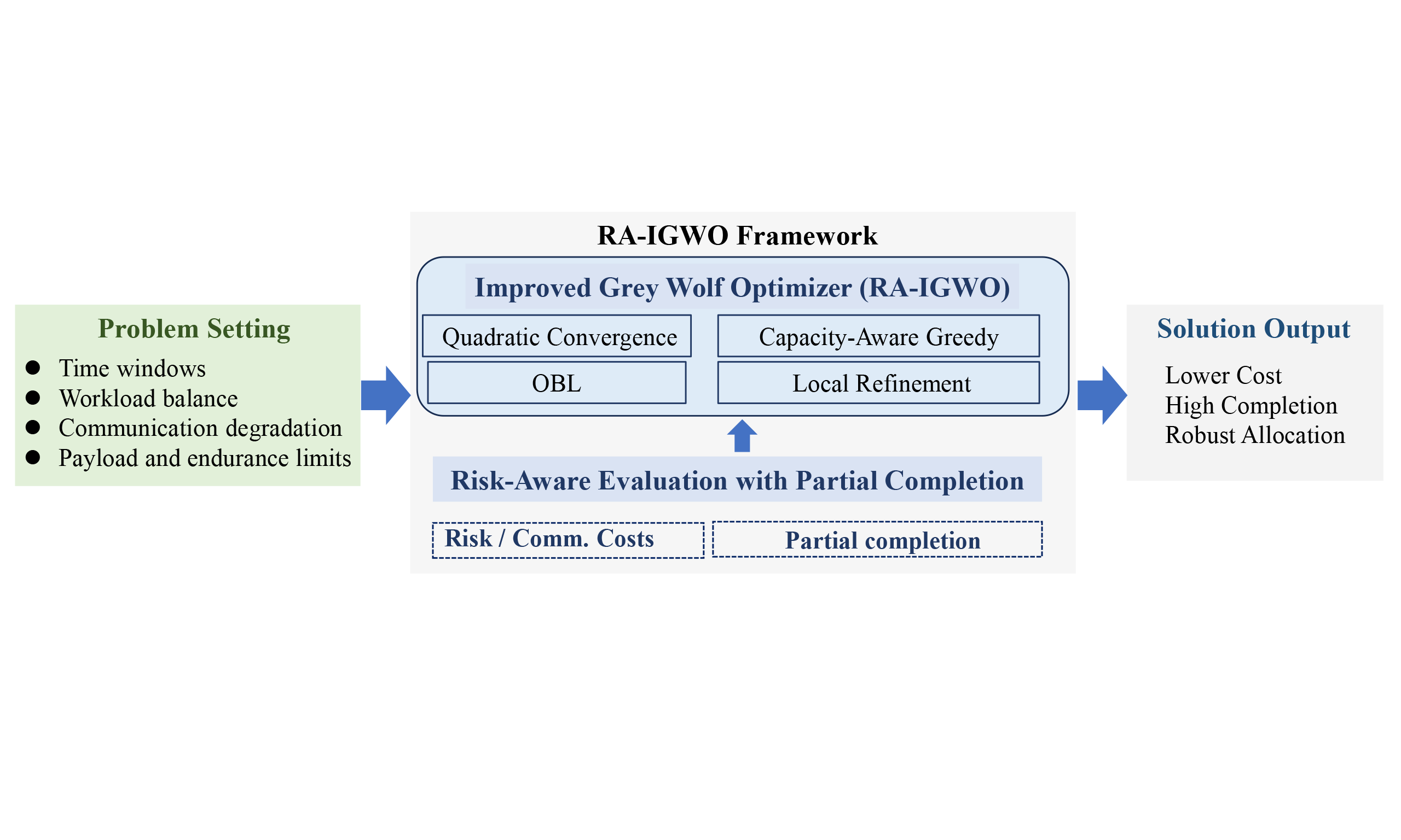
This paper investigates risk-aware task allocation for heterogeneous multi-UAV systems under coupled communication, time-window, workload, spatial-risk, payload, and endurance constraints. Existing formulations may exclude useful traversable routes or underestimate executable service by treating hazardous regions as hard barriers or using all-or-nothing feasibility evaluation. To address these limitations, a risk-aware improved Grey Wolf Optimizer (RA-IGWO) is developed within a partial-completion framework. Risk-prone and communication-degraded regions are modeled as traversable soft-cost areas, while physical obstacles are explicitly penalized and additionally examined under hard-obstacle enforcement. RA-IGWO integrates capacity-aware initialization, opposition-based learning, decoded-space local refinement, and accept-only-improved population updates. The quadratic schedule is retained only as an exploration policy rather than an independently beneficial component. All algorithms are evaluated under the same global number of fitness evaluations budget, with every candidate evaluation counted toward that budget. Experiments on independently generated instances show that RA-IGWO achieves lower objective values than five population-based baselines and remains competitive with a recent discrete adaptive large neighborhood search benchmark method. Robustness analyses show that the conclusions are not tied to a single decoder, obstacle treatment, or objective setting.
Keywords


 Download PDF
1. INTRODUCTION
Unmanned aerial vehicle (UAV) swarms are increasingly used in large-scale reconnaissance, medical-supply delivery, environmental monitoring, and post-disaster response [1,2]. Compared with homogeneous fleets, heterogeneous UAV fleets combine different cruise speeds, payload capacities, and endurance limits, thereby supporting broader coverage and diverse payload requirements. These advantages depend on a central decision problem: allocating spatially distributed tasks to available UAVs while satisfying physical and operational constraints. Multi-UAV task allocation (MUTA) is NP-hard, and its solution complexity grows rapidly with the numbers of tasks and UAVs [3,4].
Existing MUTA methods can be broadly grouped into three paradigms. Centralized exact methods, including mixed-integer programming formulations, can provide optimal solutions for small instances, but their computational burden increases rapidly with problem size and limits their use in time-sensitive missions. The consensus-based bundle algorithm is representative of decentralized market and consensus methods. During bundle construction, agents select tasks independently according to local marginal gains; during consensus, conflicts are resolved through asynchronous exchange of winner lists and timestamps without a central computing node [5,6]. Recent extensions have considered heterogeneous swarms with task-coupling constraints [7,8] and dynamic reallocation under emergent task changes [8]. Although these methods are scalable and robust, their solution quality depends strongly on bidding and scoring rules, and degraded communication can reduce coordination quality.
Swarm intelligence and evolutionary metaheuristics provide another approach to task allocation, including genetic algorithms[9,10], particle swarm optimization (PSO)[11], differential evolution[12], ant colony optimization (ACO)[13], and artificial bee colony (ABC) optimization[14]. These methods do not require gradient information and can accommodate mixed discrete and continuous structures through suitable encoding and decoding. Recent examples include multi-objective ACO for heterogeneous UAV task allocation[15] and reinforcement-learning-enhanced ABC for cooperative unmanned-helicopter scheduling[16]. The no-free-lunch theorem implies that no metaheuristic dominates across all problem classes[17], motivating algorithms that exploit the structure of a particular task domain. Recent studies have increasingly considered the coupling of UAV decision-making with communication, energy, and low-altitude obstacle constraints. For example, secure aerial communication in low-altitude intelligent networks with mixed obstacles has been investigated in[18], while joint task allocation and power optimization has been formulated as an overlapping coalition-formation problem in[19]. Furthermore, adaptive operator selection using a dueling deep Q-network has been studied in evolutionary optimization[20]. These studies advance communication optimization, decision frameworks, or adaptive operator selection, but do not explicitly address the coupled effects of risk exposure, capacity-limited execution, and many-to-one decoded allocation structures in risk-aware MUTA.
The Grey Wolf Optimizer (GWO)[21] has received substantial attention because of its simple control structure and multi-leader search mechanism. Its compact formulation facilitates hybridization[22] and has supported applications in multi-robot search and exploration[23]. However, standard GWO may converge prematurely in rugged and strongly constrained search spaces. Therefore, several GWO variants have been developed to improve convergence and population diversity in complex engineering optimization problems[24,25,26]. In MUTA, this challenge is intensified by discrete decoding boundaries and the interaction among capacity-related service loss, route exposure, and task-omission penalties. Existing variants introduce mechanisms such as Lévy flight perturbation[27], chaotic initialization[25,28], opposition-based learning (OBL)[29,30], dimension-learning-based hunting[24], PSO-GWO hybridization[31,32], and GWO–symbiotic organisms search hybridization for UAV path planning[33]. Most of these improvements target general continuous optimization and primarily modify search operators or population diversity. Risk-aware MUTA additionally requires mechanisms that account for discrete decoding, capacity-limited service, and allocation-level interactions.
Many existing MUTA studies adopt an all-or-nothing feasibility rule, under which a route is considered infeasible once its payload or endurance limit is exceeded. This treatment can over-penalize marginal violations because tasks completed before the first violation may remain physically executable. The present study instead evaluates the feasible prefix of each decoded route. A second methodological issue concerns computational fairness. Metaheuristics with embedded local search or auxiliary candidate generation may consume more fitness evaluations than conventional population updates. Comparisons based only on an equal number of generations can therefore provide such methods with a larger effective evaluation budget. To avoid this bias, all algorithms terminate under the same global number of fitness evaluation (NFE) budget.
The above analysis reveals three coupled difficulties in risk-aware MUTA. First, continuous metaheuristic updates can become ineffective after many-to-one integer decoding. Second, payload- and endurance-limited execution makes solution quality depend not only on task ownership but also on how partial service is evaluated. Third, risk and communication exposure must be balanced against task completion. These characteristics motivate an integrated design in which global exploration, structured initialization, decoded-space refinement, and risk-aware partial-completion evaluation address different but interacting aspects of the same allocation problem.
Based on the above analysis, this paper develops risk-aware improved Grey Wolf Optimizer (RA-IGWO) for risk-aware MUTA in complex environments. The framework is designed around the structure of the decoded allocation landscape rather than as a general-purpose collection of search operators. The main contributions are summarized as follows:
1. A risk-aware execution model is formulated in which risk-prone and weak-communication zones are treated as traversable soft-cost regions. Physical obstacles are explicitly distinguished and validated under both finite-penalty and hard-constraint settings. A partial-completion rule evaluates the executable prefix of each decoded UAV route under payload and endurance limits.
2. RA-IGWO is designed for the many-to-one decoded assignment landscape by combining capacity-aware greedy seeding and OBL with allocation-level load-aware local refinement and accept-only-improved population updates. Local refinement acts directly on discrete task ownership and can cross plateaus that remain unchanged under small continuous perturbations. The quadratic schedule is treated as a tested exploration policy.
3. A budget-consistent benchmarking protocol is established in which every candidate evaluation generated by population updates, OBL, or local refinement consumes one evaluation from the same global NFE budget. Then the comparisons are examined using paired multi-instance statistics and robustness analyses.
2. SYSTEM MODEL AND OPTIMIZATION FORMULATION
2.1 Mission model and assignment representation
Consider a heterogeneous fleet
The environment contains three types of circular zones. A zone
The formulation is based on five assumptions. First, each flight route is a straight segment traversed at constant speed
Principal notation
| Symbol | Meaning |
| Set of UAVs and its cardinality | |
| Set of tasks and its cardinality | |
| Position of the base and of task | |
| Reward, payload demand, and latest service time of task | |
| Speed, payload capacity, and endurance of UAV | |
| Risk-prone, weak-communication, and obstacle zones | |
| Assignment vector; UAV assigned to task | |
| Continuous search vector and per-coordinate bounds | |
| Tasks assigned to UAV | |
| Pairwise Euclidean distance matrix | |
| Risk-overlap matrix and obstacle-intersection matrix | |
| Cumulative outbound service distance of UAV | |
| Arrival time at served task | |
| Scalarized objective to be minimized | |
| Fitness-evaluation counter and evaluation budget | |
| Population size | |
| GWO convergence factor | |
| Center and radius of zone | |
| Payload-based capacity ceiling on completion rate in Eq. (12) |
The decision variable is an assignment vector
where
Motivated by threat-perception-based UAV path planning, candidate paths are evaluated using predefined exposure and feasibility costs[36]. Several geometric quantities that depend only on the static environment can therefore be precomputed. The augmented node set is
To calculate the elementwise values of
Aggregating over zones gives
Weak communication represents degradation in link reliability rather than a direct physical hazard. Its overlap coefficient is therefore set to one half of the unit coefficient assigned to the risk-zone term. The quantity
Constructing
2.2 Partial-completion service, risk-aware objective, and fitness evaluation
For an allocation vector
For the decoder-sensitivity analysis, the alternative risk-aware ordering selects the next task according to
where
Given the visiting order
If either condition is violated, the UAV terminates its service, and all subsequent tasks in
Compared with an all-or-nothing feasibility rule, prefix evaluation preserves credit for tasks completed before the first payload or endurance violation. Under an all-or-nothing rule, a small downstream violation can invalidate an entire assigned route even when several preceding tasks remain physically executable. Therefore, the present model scores the feasible prefix
The overall objective function jointly accounts for travel efficiency, environmental exposure, time-window violations, workload balance, and task reward. For each flight segment served within the feasible prefix
where
Equations (2)-(3) and (5)-(10) are derived in this study from segment-circle geometry and the stated mission assumptions. Equation (1) follows the cited round-and-clip encoding practice.
Following the standard principle of decomposing multiple criteria into a scalar optimization objective[37], the objective to be minimized is
The fixed weights are
In the experimental scenarios, it may not be possible to achieve 100% completion when the total task demand exceeds the total payload capacity of the UAV swarm. Therefore, a payload-only upper bound on the number of serviceable tasks is obtained by selecting tasks in ascending order of demand:
where
Algorithm 1 summarizes the fitness evaluation. Each call to the objective function increments the global counter
| Algorithm 1 Evaluate |
| 1: |
| 2: |
| 3: for each UAV |
| 4: |
| 5: |
| 6: for |
| 7: |
| 8: if |
| 9: |
| 10: |
| 11: |
| 12: |
| 13: else |
| 14: break ▷stop the UAV; remaining tasks in |
| 15: end if |
| 16: end for |
| 17: |
| 18: end for |
| 19: |
| 20: return |
3. RA-IGWO for Risk-Aware UAV Task Allocation
The decoded task-allocation problem produces a rugged fitness landscape in which objective values are jointly affected by payload violations, task omissions, route exposure, and workload imbalance. Continuous GWO updates do not always change the decoded assignment, which can promote stagnation on the many-to-one decoding plateaus. The implemented optimizer uses a quadratic convergence schedule, capacity-aware greedy initialization, OBL, allocation-level load-aware local refinement, and accept-only-improved population updates. All candidate fitness evaluations generated by population updates, OBL, and local refinement are counted against the same global budget
3.1 Standard GWO update and quadratic convergence schedule
In standard GWO[21], the population is ranked by fitness, and the three best agents are denoted by
where
Since each component of
In standard GWO,
while retaining the three-leader update in Eq. (13). For
3.2 Capacity-aware greedy initialization, OBL, and local refinement
The remaining components are designed around the decoded assignment structure. During initialization,
OBL[29] is used to expand the sampling area of the continuous search space. The opposite solution of a proxy
After evaluating the opposite candidates at initialization, the best
The alpha wolf is further refined by first-improvement search in the decoded integer space. The search samples three neighborhood types: load-aware transfer, reassignment, and two-task swapping. The load-aware transfer moves a task from the most capacity-constrained UAV to a UAV with larger remaining capacity to reduce service loss caused by payload limits, while the other operations maintain neighborhood diversity. Each sampled local-refinement candidate is evaluated by Algorithm 1 and consumes one NFE regardless of whether it improves the incumbent solution. This rule prevents local search from receiving an uncounted evaluation advantage over non-memetic baselines.
3.3 Overall RA-IGWO procedure and evaluation-budget accounting
Algorithm 2 summarizes the complete optimizer. Greedy seeding, OBL refresh, GWO position updates, and assignment-level local refinement all follow the same NFE accounting rule. After local refinement, the alpha solution is written back to the population before the leaders are updated again; otherwise, the refined assignment could be lost during the next population ranking.
| Algorithm 2 RA-IGWO with embedded greedy seeding and local refinement |
| 1: Input: evaluation budget |
| 2: |
| 3: evaluate all agents by Algorithm 1; evaluate opposite agents by Eq. (15); retain the best |
| 4: while |
| 5: set |
| 6: if |
| 7: perform generalized OBL using current population bounds; evaluate opposite agents and retain the best |
| 8: end if |
| 9: update leaders; decode the current alpha wolf as |
| 10: refine ▷each evaluated local candidate consumes one NFE regardless of acceptance |
| 11: write the refined leader back to the population, |
| 12: end while |
| 13: return |
4. SIMULATION RESULTS AND ROBUSTNESS ANALYSIS
Experiments use Python 3.12.0 on an Intel Core i9-13900HX workstation with 16GB RAM and no algorithm-level parallelism. All plots and route visualizations are author-generated from the reported outputs using Python, NumPy, and Matplotlib.
RA-IGWO is compared with GA, PSO, GWO, I-GWO, HPSOGWO, and a discrete adaptive large neighborhood search benchmark (D-ALNS). Representative and hard-obstacle tests use
4.1 Experimental setup and fairness protocol
All methods follow one evaluation protocol. Table 2 lists all settings. Every RA-IGWO candidate produced by a GWO update, OBL refresh, or local refinement consumes one NFE; the final diagnostic call reports metrics only. Reference configurations are used for GA[9,10], PSO[38,39,11], GWO[21], I-GWO[24], HPSOGWO[31,32], and UAV multi-task ALNS[40]. D-ALNS adapts the latter framework to ownership-only decisions. Its random, worst-contribution, overload-oriented, and risk-oriented removal operators are paired with greedy, regret-2, and capacity-balanced repair, adaptive operator weights, and simulated-annealing acceptance. Each repaired assignment consumes one NFE. GWO uses
Algorithm and environment parameters
| Component | Parameter | Value | Parameter | Value |
| All methods | NFE budget | 4, 000 | Independent instances/seeds | 20/5 |
| Population methods | Pop size | 30 | Boundary handling | Clipping |
| GA | Crossover prob. | 0.80 | Mutation prob. | 0.10 |
| PSO | Inertia | 0.70 | Accel. | 1.5, 1.5 |
| HPSOGWO | Coeff. ( | 0.5, 0.5, 0.5, 0.5 | – | – |
| D-ALNS | Destroy fractions | 0.10, 0.20, 0.30 | Reaction/cooling | 0.20/0.999 |
| RA-IGWO | Jump rate | 0.30 | Greedy seed count | |
| Environment | Area side | 100 | Task position | |
| UAV speed | UAV payload | |||
| UAV range | Task demand | |||
| Task reward | Tasks with time windows | |||
| Deadline | Obstacle zones | 2 | ||
| Weak-comm. zones | 2 | Zone radius (risk/comm.) | ||
| Zone radius (obstacle) | – | – | ||
| Fitness weights | 1, 2, 3, 0.5, 1 | 80, 500 |
With
Runtime covers optimizer construction and search. Environment generation, geometric preprocessing, output, visualization, and the post-run diagnostic call are excluded, yielding implementation-level comparisons in a common environment.
Table 3 examines GA, PSO, and GWO parameters under the common population and NFE settings; it is a sensitivity analysis, not independent optimization. Mean fitness spans 2, 198.69-3, 500.42 for GA, 2, 019.49-2, 436.36 for PSO, and 2, 055.63-2, 414.42 for GWO, so the predeclared settings are treated as reproducible rather than optimal. The strongest observed configurations are then tested on 20 new environments with five paired seeds. I-GWO and HPSOGWO retain their reference implementations. In Table 4, RA-IGWO obtains mean fitness 1, 688.91
Parameter sensitivity of GA, PSO, and GWO on medium-scale instances under the shared 4000-NFE budget
| Algorithm | Parameter setting | Runs | Fitness mean | Completion |
| GA | 10 | 68.6% | ||
| GA | 10 | 68.4% | ||
| GA | 10 | 71.6% | ||
| GA | 10 | 74.4% | ||
| GA | 10 | 69.0% | ||
| PSO | 10 | 74.2% | ||
| PSO | 10 | 73.6% | ||
| PSO | 10 | 76.4% | ||
| PSO | 10 | 71.8% | ||
| PSO | 10 | 68.6% | ||
| GWO | 10 | 70.0% | ||
| GWO | 10 | 73.8% | ||
| GWO | 10 | 69.6% | ||
| GWO | 10 | 67.8% |
Confirmation using the strongest observed GA, PSO, and GWO settings on independent medium-scale instances
| Algorithm | Confirmation setting | Runs | Fitness mean | Completion | FDR |
| GA | 100 | 73.0% | |||
| PSO | 100 | 75.0% | |||
| GWO | 100 | 70.9% | |||
| I-GWO | Reference implementation | 100 | 68.4% | ||
| HPSOGWO | Reference implementation | 100 | 70.1% | ||
| RA-IGWO | Proposed configuration | 100 | 83.6% | – |
4.2 Representative main comparison
Table 5 gives one reproducible 4000-NFE run to illustrate distance, risk, completion, balance, and runtime jointly.
Representative single-run performance under a 4000-NFE budget
| Scenario | Algorithm | Fitness | Distance | Risk | #Tardy | Completion | Cap. | Balance | Time (s) |
| Small | GA | 1, 835.79 | 658.7 | 110.6 | 0 | 76.7% | 93.3% | 51.49 | 0.64 |
| Small | PSO | 1, 528.85 | 589.7 | 122.4 | 0 | 86.7% | 38.30 | 0.56 | |
| Small | GWO | 1, 152.92 | 534.4 | 43.2 | 0 | 73.3% | 36.83 | 0.62 | |
| Small | I-GWO | 1, 072.82 | 594.8 | 99.8 | 0 | 83.3% | 51.59 | 0.66 | |
| Small | HPSOGWO | 1, 374.89 | 533.6 | 109.2 | 0 | 70.0% | 59.27 | 0.67 | |
| Small | RA-IGWO | 893.03 | 569.1 | 108.8 | 0 | 90.0% | 38.72 | 0.65 | |
| Medium | GA | 2, 470.62 | 835.1 | 145.2 | 0 | 62.0% | 88.0% | 47.08 | 0.96 |
| Medium | PSO | 2, 801.34 | 971.4 | 127.2 | 0 | 80.0% | 40.81 | 0.89 | |
| Medium | GWO | 2, 065.81 | 914.6 | 119.6 | 0 | 72.0% | 28.78 | 0.94 | |
| Medium | I-GWO | 2, 844.55 | 608.9 | 95.0 | 0 | 46.0% | 43.73 | 0.99 | |
| Medium | HPSOGWO | 2, 582.86 | 722.2 | 166.4 | 0 | 58.0% | 54.18 | 0.99 | |
| Medium | RA-IGWO | 1, 987.10 | 780.4 | 73.6 | 0 | 80.0% | 31.20 | 0.95 | |
| Large | GA | 4, 549.23 | 1, 114.6 | 510.7 | 1 | 58.8% | 80.0% | 36.44 | 1.41 |
| Large | PSO | 3, 903.63 | 1, 038.3 | 370.1 | 0 | 62.5% | 30.18 | 1.40 | |
| Large | GWO | 4, 344.36 | 1, 164.5 | 427.0 | 2 | 60.0% | 39.10 | 1.39 | |
| Large | I-GWO | 5, 162.62 | 1, 155.8 | 562.8 | 0 | 58.8% | 18.36 | 1.49 | |
| Large | HPSOGWO | 4, 815.38 | 1, 032.7 | 535.2 | 0 | 53.8% | 42.17 | 1.48 | |
| Large | RA-IGWO | 3, 228.84 | 1, 053.0 | 357.7 | 0 | 72.5% | 27.51 | 1.46 |
RA-IGWO has the lowest fitness and highest or tied-highest completion in all three representative runs. Figure 1 visualizes the large-scale metric decomposition. Because one run is descriptive rather than inferential, robustness is assessed below using independent instances, confidence intervals, effect sizes, and sensitivity tests.
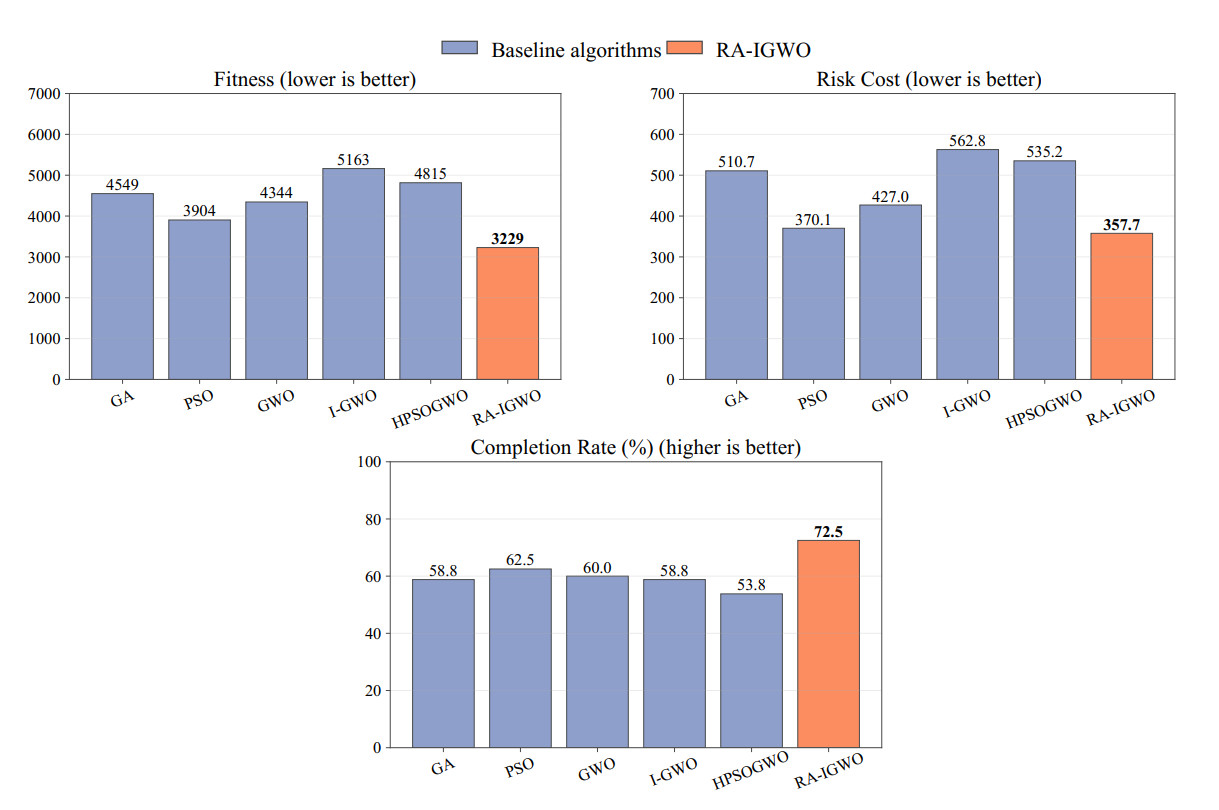
Figure 1. Large-scale representative metric comparison under the shared 4000-NFE budget. Blue bars denote baseline algorithms, and orange bars denote RA-IGWO. Bold value labels denote the best result in each panel, namely the lowest fitness and risk cost and the highest completion rate.
4.3 Convergence behavior
Figure 2 plots best-so-far fitness against NFE for all three representative scales. Capacity-aware seeding structures initial allocations, OBL broadens sampling, and the quadratic schedule prolongs the interval with
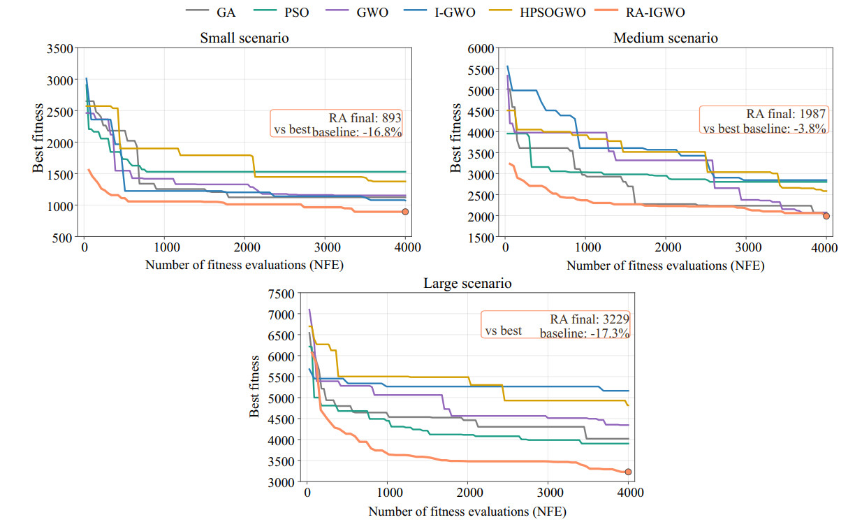
Figure 2. Convergence curves under the shared NFE budget for small, medium, and large-scale scenarios.
4.4 Obstacle-model validation
Because a finite penalty can permit crossings, Table 6 reports mean intersections over 20 environments and five seeds per method and instance. RA-IGWO ranks first in the medium and large cases and second in the small case. These results quantify penalized soft-obstacle behavior and must not be interpreted as strict avoidance.
Obstacle-intersection statistics under the default soft-obstacle formulation
| Scenario | GA | PSO | GWO | I-GWO | HPSOGWO | RA-IGWO |
| Small-20 | 0.32 | 0.37 | 0.31 | 0.26 | 0.34 | 0.29 |
| Medium-50 | 0.72 | 0.10 | 0.15 | 0.06 | 0.15 | 0.03 |
| Large-100 | 1.36 | 0.12 | 0.35 | 0.33 | 0.30 | 0.10 |
Table 7 enforces hard obstacles. A task
Hard-obstacle validation for the six population-based algorithms
| Scenario | Algorithm | Fitness mean | Completion | Crossings | Runtime (s) |
| Small | GA | 1, 192.60 | 72.6% | 0.00 | 0.686 |
| Small | PSO | 1, 022.73 | 79.1% | 0.00 | 0.646 |
| Small | GWO | 1, 023.95 | 77.9% | 0.00 | 0.721 |
| Small | I-GWO | 1, 036.32 | 78.0% | 0.00 | 0.754 |
| Small | HPSOGWO | 1, 048.90 | 77.7% | 0.00 | 0.741 |
| Small | RA-IGWO | 918.47 | 82.0% | 0.00 | 0.724 |
| Medium | GA | 2, 293.60 | 67.0% | 0.00 | 1.026 |
| Medium | PSO | 1, 806.23 | 77.8% | 0.00 | 0.998 |
| Medium | GWO | 2, 009.40 | 73.1% | 0.00 | 1.071 |
| Medium | I-GWO | 2, 103.02 | 71.5% | 0.00 | 1.099 |
| Medium | HPSOGWO | 2, 082.71 | 71.9% | 0.00 | 1.087 |
| Medium | RA-IGWO | 1, 559.83 | 83.2% | 0.00 | 1.090 |
| Large | GA | 4, 431.34 | 52.1% | 0.00 | 1.581 |
| Large | PSO | 3, 680.88 | 61.7% | 0.00 | 1.539 |
| Large | GWO | 4, 049.59 | 56.8% | 0.00 | 1.619 |
| Large | I-GWO | 4, 224.20 | 54.4% | 0.00 | 1.658 |
| Large | HPSOGWO | 4, 195.09 | 55.2% | 0.00 | 1.637 |
| Large | RA-IGWO | 3, 264.90 | 66.4% | 0.00 | 1.685 |
Table 8 varies
Cross-algorithm obstacle-penalty sensitivity on medium-scale instances
| PSO fitness | RA-IGWO fitness | RA completion | RA crossings | FDR | |
| 100 | 1, 921.20 | 1, 679.54 | 82.8% | 0.66 | |
| 250 | 2, 009.85 | 1, 716.62 | 82.4% | 0.35 | |
| 500 | 2, 059.88 | 1, 809.21 | 82.4% | 0.32 | 0.0003 |
| 1, 000 | 2, 249.11 | 1, 964.54 | 81.9% | 0.30 | |
| 2, 000 | 2, 520.28 | 2, 121.70 | 82.2% | 0.24 |
4.5 Decoder sensitivity
Table 9 applies four decoders to all six population methods over 20 medium-scale instances and five seeds. Risk-aware ordering reduces RA-IGWO fitness from 1, 766.47 to 1, 600.78 and eliminates obstacle crossings. For RA-IGWO, skip-and-continue increases completion from 84.8% to 85.3% under nearest-neighbor ordering and leaves completion unchanged at 85.3% under risk-aware ordering. For PSO, completion changes slightly from 78.1% to 78.0% and from 80.7% to 80.3%, respectively. The completion effect of skipping is small and method-dependent. PSO is the strongest population-based baseline for each decoder, while RA-IGWO retains lower fitness than all five population-based baselines under every decoder, with all 20 joint FDR-adjusted comparisons significant (
Cross-algorithm decoder sensitivity on medium-scale instances
| Decoder | PSO fitness | RA fitness | PSO comp. | RA comp. | RA crossings | FDR |
| NN-stop | 2, 124.53 | 1, 766.47 | 78.1% | 84.8% | 0.42 | |
| Risk-stop | 1, 830.91 | 1, 600.78 | 80.7% | 85.3% | 0.00 | |
| NN-skip | 2, 122.80 | 1, 757.47 | 78.0% | 85.3% | 0.36 | |
| Risk-skip | 1, 869.79 | 1, 597.60 | 80.3% | 85.3% | 0.00 |
4.6 Objective-scale, weight, and normalization sensitivity
Objective-scale robustness is examined through empirical term magnitudes, common weight profiles, and normalization. Across 2, 000 random medium-scale assignments, median absolute weighted contributions for distance, risk, delay, imbalance, reward, missed tasks, and obstacles are 1, 051.25, 727.50, 84.85, 19.82, 196.74, 1, 040.00, and 3, 000.00. The dominant missed-task and obstacle terms motivate the checks below. Because each profile defines a different scalar objective, raw fitness is compared within a common profile.
Table 10 reports objective-weight sensitivity. The three-profile comparison and separate five-level
Cross-algorithm objective-weight profiles on medium-scale instances
| Profile | PSO fitness | RA fitness | RA completion | RA risk | RA crossings | FDR |
| Completion-oriented | 1, 901.72 | 1, 658.34 | 84.0% | 203.70 | 0.54 | 0.0020 |
| Balanced | 2, 154.68 | 1, 874.05 | 82.9% | 141.57 | 0.53 | |
| Risk-oriented | 2, 904.99 | 2, 426.16 | 77.2% | 80.71 | 0.48 |
For normalized-objective testing, distance, risk, delay, balance, reward, missed-task, and obstacle terms are divided by scales
where tasks with infinite deadlines are excluded and contribute zero delay. If no finite deadline exists, the inner maximum is defined as zero, giving
All-algorithm comparison under the normalized objective
| Algorithm | Fitness mean | Completion | Crossings | Runtime (s) |
| GA | 75.2% | 0.82 | 1.191 | |
| PSO | 84.2% | 0.22 | 1.142 | |
| GWO | 79.2% | 0.35 | 1.230 | |
| I-GWO | 77.9% | 0.23 | 1.273 | |
| HPSOGWO | 78.7% | 0.23 | 1.262 | |
| D-ALNS | 86.2% | 0.14 | 4.316 | |
| RA-IGWO | 86.5% | 0.18 | 1.194 |
4.7 Multi-instance generalization and statistical evidence
Each Small-20, Medium-50, and Large-100 setting uses 20 independently generated instances and five seeds per method and instance. The environment is the statistical unit: seeds are averaged within an instance before paired inference. For each environment and seed index, the same integer seed is reset before every algorithm. Table 12 reports the strongest population comparator, D-ALNS, and RA-IGWO; Table 13 covers all seven methods with Benjamini-Hochberg correction jointly applied across 18 comparisons.
Multi-instance generalization summary
| Scenario | Algorithm | Fitness mean | Completion | Crossings | Runtime (s) |
| Small-20 | I-GWO | 790.56 | 88.8% | 0.26 | 0.735 |
| Small-20 | D-ALNS | 1, 042.09 | 98.2% | 1.02 | 1.839 |
| Small-20 | RA-IGWO | 709.30 | 94.4% | 0.29 | 0.671 |
| Medium-50 | PSO | 1, 970.25 | 76.6% | 0.10 | 1.202 |
| Medium-50 | D-ALNS | 1, 695.54 | 82.1% | 0.09 | 4.474 |
| Medium-50 | RA-IGWO | 1, 608.30 | 83.0% | 0.03 | 1.178 |
| Large-100 | PSO | 5, 092.63 | 53.7% | 0.12 | 2.097 |
| Large-100 | D-ALNS | 4, 642.23 | 55.0% | 0.00 | 11.233 |
| Large-100 | RA-IGWO | 4, 564.23 | 56.8% | 0.10 | 2.287 |
FDR-adjusted paired Wilcoxon evidence for RA-IGWO versus all baselines
| Scenario | Baseline | FDR | RA better | ||
| Small-20 | GA | 244.76 [203.58, 292.97] | 2.359 | 100% | |
| Small-20 | PSO | 119.34 [82.06, 164.96] | 1.218 | 100% | |
| Small-20 | GWO | 104.20 [86.11, 124.42] | 2.335 | 100% | |
| Small-20 | I-GWO | 81.26 [60.91, 102.37] | 1.678 | 100% | |
| Small-20 | HPSOGWO | 123.72 [103.50, 147.34] | 2.410 | 100% | |
| Small-20 | D-ALNS | 332.78 [188.08, 499.71] | 0.0010 | 0.902 | 70% |
| Medium-50 | GA | 1, 272.26 [1160.22, 1385.95] | 4.741 | 100% | |
| Medium-50 | PSO | 361.95 [311.67, 411.38] | 3.074 | 100% | |
| Medium-50 | GWO | 682.30 [604.85, 770.83] | 3.464 | 100% | |
| Medium-50 | I-GWO | 808.74 [738.66, 892.07] | 4.541 | 100% | |
| Medium-50 | HPSOGWO | 731.28 [652.85, 819.02] | 3.768 | 100% | |
| Medium-50 | D-ALNS | 87.23 [19.03, 178.47] | 0.0121 | 0.460 | 65% |
| Large-100 | GA | 1, 916.12 [1652.70, 2183.74] | 3.062 | 100% | |
| Large-100 | PSO | 528.40 [463.71, 595.78] | 3.420 | 100% | |
| Large-100 | GWO | 1, 098.73 [935.24, 1258.21] | 2.874 | 100% | |
| Large-100 | I-GWO | 1, 248.65 [1096.16, 1405.13] | 3.392 | 100% | |
| Large-100 | HPSOGWO | 1, 169.16 [1006.94, 1339.54] | 2.938 | 100% | |
| Large-100 | D-ALNS | 78.01 [ | 0.0113 | 0.462 | 75% |
Relative to D-ALNS, RA-IGWO reduces mean fitness by 332.78, 87.23, and 78.01 at the three scales, with significant FDR-adjusted signed-rank tests. However, for Large-100, the bootstrap CI
Table 14 shows scale-dependent hard-obstacle results: D-ALNS is significantly better for Small-30 and Medium-50, but RA-IGWO is better for Large-80. Under normalization they are statistically indistinguishable. Thus, RA-IGWO remains superior to the five population baselines under hard obstacles but not uniformly to the discrete baseline. Separate medium-scale D-ALNS sensitivity checks vary destroy fraction, reaction factor, and cooling rate, and none differs significantly from the predeclared configuration after FDR correction. Figure 3 displays all seven methods across the three multi-instance scales.
Matched robustness comparison with the discrete D-ALNS baseline
| Setting | D-ALNS fitness | RA-IGWO fitness | D-ALNS comp. | RA-IGWO comp. | FDR | |
| Hard, Small-30 | 82.7% | 82.0% | ||||
| Hard, Medium-50 | 83.6% | 83.2% | ||||
| Hard, Large-80 | 65.1% | 66.4% | 0.0064 | |||
| Normalized, Medium-50 | 86.2% | 86.5% | 0.4524 |
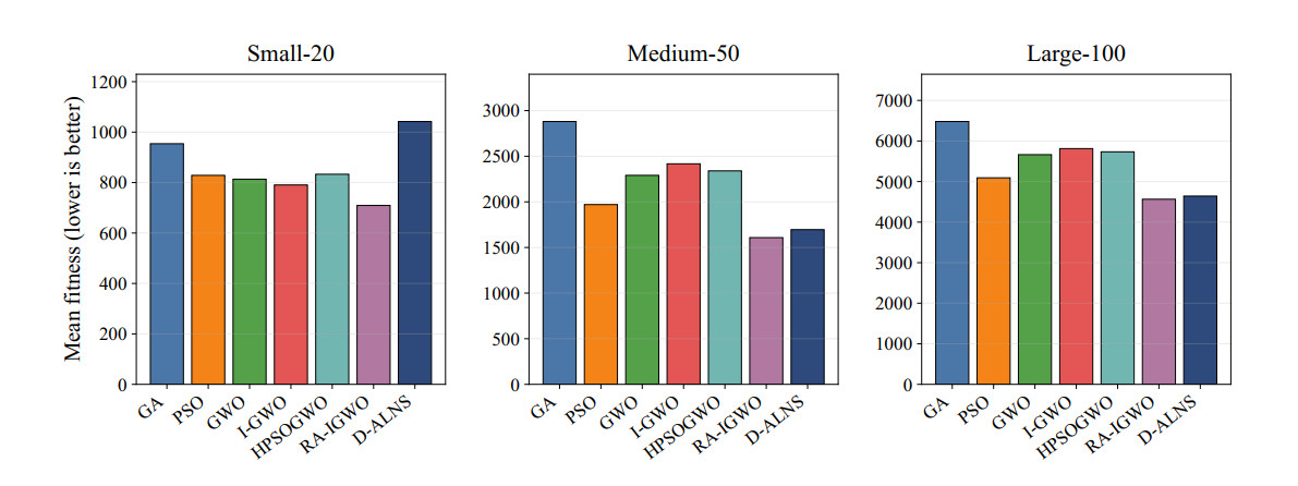
Figure 3. Mean fitness over independently generated spatial instances.
4.8 Component ablation
Table 15 uses 20 medium instances and isolates each component. Removing local refinement or accept-only updates raises fitness by 740.46 and 480.55, respectively, with FDR significance. Greedy initialization has mixed evidence:
Multi-instance leave-one-component-out and elitist-update ablation
| Variant | Fitness mean | FDR | Completion | |
| Full | – | – | 83.7% | |
| Without greedy | 0.0551 | 84.1% | ||
| Without OBL | 0.0826 | 84.2% | ||
| Without quadratic | 0.0399 | 84.0% | ||
| Without local | 740.46 [672.94, 804.84] | 69.7% | ||
| Without elitist update | 480.55 [387.45, 581.25] | 76.4% |
The interaction study likewise shows no quadratic-schedule gain: fitness changes from 2, 514.06 to 2, 539.65 without local refinement and from 1, 764.72 to 1, 780.56 with it. Accordingly, only local refinement and elitist acceptance receive clear support; greedy evidence is mixed and OBL is independently non-significant.
4.9 Return-to-base validation
Excluding return travel can overestimate endurance feasibility. Table 16 and Figure 4 therefore compare outbound-only and return-guaranteed evaluation for all six population methods. RA-IGWO has the lowest mean fitness and highest completion in both modes, preserving its population-baseline ranking under the more conservative endurance model.
Outbound-only and return-guaranteed endurance evaluation
| Mode | Algorithm | Fitness mean | Completion | Crossings |
| Outbound-only | GA | 3, 164.31 | 72.1% | 1.35 |
| Outbound-only | PSO | 2, 067.72 | 77.3% | 0.25 |
| Outbound-only | GWO | 2, 305.66 | 71.9% | 0.15 |
| Outbound-only | I-GWO | 2, 526.55 | 70.5% | 0.20 |
| Outbound-only | HPSOGWO | 2, 442.39 | 69.7% | 0.25 |
| Outbound-only | RA-IGWO | 1, 686.17 | 85.8% | 0.20 |
| Return-guaranteed | GA | 3, 048.62 | 72.1% | 1.00 |
| Return-guaranteed | PSO | 2, 078.84 | 78.1% | 0.30 |
| Return-guaranteed | GWO | 2, 435.93 | 72.3% | 0.35 |
| Return-guaranteed | I-GWO | 2, 570.15 | 68.7% | 0.25 |
| Return-guaranteed | HPSOGWO | 2, 363.09 | 70.4% | 0.25 |
| Return-guaranteed | RA-IGWO | 1, 659.22 | 85.9% | 0.15 |
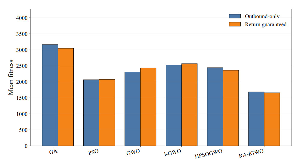
Figure 4. Effect of adding return-to-base feasibility to the endurance evaluation.
4.10 Visualization, practical relevance, and limitations
Figure 5 shows representative allocations and routes and should be read with the intersection statistics; under the soft model, crossings are penalized and reported rather than forbidden. The model addresses offline low-altitude allocation with mixed obstacles, communication degradation, and limited resources[18,19], focusing on risk-aware ownership, route-prefix feasibility, and unified-NFE evaluation rather than communication-centric power allocation.
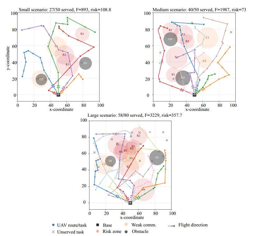
Figure 5. RA-IGWO task allocation and routes for the three scenarios. The black box marked "H" denotes the common home base (takeoff and landing pad).
Future work will consider dynamically changing maps, online replanning, adaptive learning of objective weights, and comprehensive automatic tuning under equal budgets.
5. CONCLUSIONS
This paper proposed RA-IGWO for risk-aware heterogeneous MUTA under coupled spatial, communication, payload, endurance, and time-window constraints. The framework combines partial-completion evaluation with decoded-space refinement and a unified fitness-evaluation budget. Multi-instance results show robust advantages over population-based baselines across decoder choices, obstacle treatments, and objective-weight settings, while comparisons with D-ALNS reveal scale- and constraint-dependent performance rather than universal superiority. Ablation results identify decoded-space local refinement and accept-only-improved updates as the main supported contributors; greedy initialization and OBL show weak or mixed independent effects, whereas the quadratic schedule is not supported as a performance-enhancing component. Future work will address adaptive scheduling, systematic parameter tuning, dynamic replanning, and adaptive multi-criteria weighting.
DECLARATIONS
Authors' contributions
Conceptualization, software, methodology, writing-original draft: Miao, X.
Validation, formal analysis, review and editing: Zhang, Z.
Data curation and visualization: Wang, Y.
Project administration, funding acquisition, review and editing: Li, B.
Availability of data and materials
The raw data supporting the conclusions of this article will be made available by the authors upon request.
AI and AI-assisted tools statement
Not applicable.
Financial support and sponsorship
This work was supported by the National Natural Science Foundation of China (62473249), Natural Science Foundation of Shanghai (23ZR1426600).
Conflicts of interest
All authors declared that there are no conflicts of interest.
Ethical approval and consent to participate
Not applicable.
Consent for publication
Not applicable.
Copyright
© The Author(s) 2026.
REFERENCES
1. Chung, S.; Paranjape, A. A.; Dames, P.; Shen, S.; Kumar, V. A survey on aerial swarm robotics. IEEE Trans. Robot. 2018, 34, 837-55.
2. Cao, Y.; Long, T.; Sun, J.; Wang, Z.; Xu, G. Comparison of distributed task allocation algorithms considering non-ideal communication factors for multi-UAV collaborative visit missions. IEEE Robot. Autom. Lett. 2025, 10, 1928-35.
3. Gerkey, B. P.; Matarić, M. J. A formal analysis and taxonomy of task allocation in multi-robot systems. Int. J. Robot. Res. 2004, 23, 939-54.
4. Chakraa, H.; Guérin, F.; Leclercq, E.; Lefebvre, D. Optimization techniques for multi-robot task allocation problems: review on the state-of-the-art. Robot Autom. Syst 2023, 168, 104492.
5. Choi, H. L.; Brunet, L.; How, J. P. Consensus-based decentralized auctions for robust task allocation. IEEE Trans. Robot. 2009, 25, 912-26.
6. Chen, J.; Qing, X.; Ye, F.; Xiao, K.; You, K.; Sun, Q. Consensus-based bundle algorithm with local replanning for heterogeneous multi-UAV system in the time-sensitive and dynamic environment. J. Supercomput. 2022, 78, 1712-40.
7. Ye, F.; Chen, J.; Sun, Q.; Tian, Y.; Jiang, T. Decentralized task allocation for heterogeneous multi-UAV system with task coupling constraints. J. Supercomput. 2021, 77, 111-32.
8. Tang, J.; Chen, X.; Zhu, X.; Zhu, F. Dynamic reallocation model of multiple unmanned aerial vehicle tasks in emergent adjustment scenarios. IEEE Trans. Aerosp. Electron. Syst. 2023, 59, 1139-55.
9. Holland, J. H. Adaptation in natural and artificial systems: an introductory analysis with applications to biology, control, and artificial intelligence. Cambridge, MA: MIT Press; 1992.
10. Tang, J.; Liu, D.; Wang, Q.; Li, J.; Sun, J. Probabilistic chain-enhanced parallel genetic algorithm for UAV reconnaissance task assignment. Drones 2024, 8, 213.
11. Phung, M. D.; Ha, Q. P. Motion-encoded particle swarm optimization for moving target search using UAVs. Appl. Soft Comput. 2020, 97, 106705.
12. Das, S.; Suganthan, P. N. Differential evolution: a survey of the state-of-the-art. IEEE Trans. Evol. Comput. 2011, 15, 4-31.
13. Dorigo, M.; Maniezzo, V.; Colorni, A. Ant system: optimization by a colony of cooperating agents. IEEE Trans. Syst. Man Cybern. B 1996, 26, 29-41.
14. Karaboga, D.; Basturk, B. A powerful and efficient algorithm for numerical function optimization: artificial bee colony (ABC) algorithm. J. Glob. Optim. 2007, 39, 459-71.
15. Chen, L.; Liu, W.; Zhong, J. An efficient multi-objective ant colony optimization for task allocation of heterogeneous unmanned aerial vehicles. J. Comput. Sci. 2022, 58, 101545.
16. Han, Z.; Chen, M.; Shao, S.; Zhu, H.; Wu, Q. Cooperative multi-task assignment of unmanned autonomous helicopters based on hybrid enhanced learning ABC algorithm. IEEE Trans. Intell. Veh. 2024, 9, 526-40.
17. Wolpert, D. H.; Macready, W. G. No free lunch theorems for optimization. IEEE Trans. Evol. Comput. 1997, 1, 67-82.
18. He, Y.; Huang, F.; Liang, Y.; et al. Sum secrecy rate enhancement in low-altitude intelligent networks with mixed obstacles. IEEE Internet Things J. 2026, 13, 29969-81.
19. Qin, Y.; Wang, Z.; Zhang, H. Joint task allocation and power optimization in multi-UAV Systems: an overlapping coalition formation game approach. IEEE Trans. Veh. Technol. 2026, 75, 1480-91.
20. Yin, S.; Xiang, Z. Adaptive operator selection with dueling deep Q-network for evolutionary multi-objective optimization. Neurocomputing 2024, 581, 127491.
21. Mirjalili, S.; Mirjalili, S. M.; Lewis, A. Grey wolf optimizer. Adv. Eng. Softw. 2014, 69, 46-61.
22. Faris, H.; Aljarah, I.; Al-Betar, M. A.; Mirjalili, S. Grey wolf optimizer: a review of recent variants and applications. Neural Comput. Applic. 2018, 30, 413-35.
23. Tang, H.; Sun, W.; Lin, A.; Xue, M.; Zhang, X. A GWO-based multi-robot cooperation method for target searching in unknown environments. Expert Syst. Appl. 2021, 186, 115795.
24. Nadimi-Shahraki, M. H.; Taghian, S.; Mirjalili, S. An improved grey wolf optimizer for solving engineering problems. Expert Syst. Appl. 2021, 166, 113917.
25. Hou, Y.; Gao, H.; Wang, Z.; Du, C. Improved Grey wolf optimization algorithm and application. Sensors 2022, 22, 3810.
26. Qiu, Y.; Yang, X.; Chen, S. An improved gray wolf optimization algorithm solving to functional optimization and engineering design problems. Sci. Rep. 2024, 14, 14190.
27. Heidari, A. A.; Pahlavani, P. An efficient modified grey wolf optimizer with lévy flight for optimization tasks. Appl. Soft Comput. 2017, 60, 115-34.
28. Saxena, A.; Kumar, R.; Das, S.
29. Tizhoosh, H. R. Opposition-based learning: a new scheme for machine intelligence. In Proceedings of the International Conference on Computational Intelligence for Modelling, Control and Automation and International Conference on Intelligent Agents, Web Technologies and Internet Commerce. IEEE; 2005. pp. 695-701.
30. Dhargupta, S.; Ghosh, M.; Mirjalili, S.; Sarkar, R. Selective opposition based grey wolf optimization. Expert Syst. Appl. 2020, 151, 113389.
31. Singh, N.; Singh, S. B. Hybrid Algorithm of particle swarm optimization and grey wolf optimizer for improving convergence performance. J. Appl. Math. 2017, 2017, 2030489.
32. Zhang, X.; Lin, Q.; Mao, W.; Liu, S.; Dou, Z.; Liu, G. Hybrid particle swarm and grey wolf optimizer and its application to clustering optimization. Appl. Soft Comput. 2021, 101, 107061.
33. Qu, C.; Gai, W.; Zhang, J.; Zhong, M. A novel hybrid grey wolf optimizer algorithm for unmanned aerial vehicle (UAV) path planning. Knowl. Based Syst. 2020, 194, 105530.
34. Martin, J. A.; Ouwerkerk, J. N.; Lamping, A. P.; Cohen, K. Comparison of battery modeling regression methods for application to unmanned aerial vehicles. Complex Eng. Syst. 2022, 2, 5.
35. Liu, J.; Wang, Y.; Xin, B.; Wang, L. A biobjective perspective for mixed-integer programming. IEEE Trans. Syst. Man. Cybern. Syst. 2022, 52, 2374-85.
36. Fu, Y.; Ding, M.; Zhou, C. Phase angle-encoded and quantum-behaved particle swarm optimization applied to three-dimensional route planning for UAV. IEEE Trans. Syst. Man Cybern. A 2012, 42, 511-26.
37. Zhang, Q.; Li, H. MOEA/D: a multiobjective evolutionary algorithm based on decomposition. IEEE Trans. Evol. Comput. 2007, 11, 712-31.
38. Kennedy, J.; Eberhart, R. Particle swarm optimization. In Proceedings of ICNN'95-International Conference on Neural Networks. IEEE; 1995. pp. 1942-48.
39. Clerc, M.; Kennedy, J. The Particle swarm-explosion, stability, and convergence in a multidimensional complex space. IEEE Trans. Evol. Comput. 2002, 6, 58-73.
Cite This Article
 Open Access
How to Cite
Miao, X.; Zhang, Z.; Wang, Y.; Li, B. A risk-aware improved grey wolf optimizer algorithm for multi-UAV task allocation in spatially constrained environments. Complex Eng. Syst. 2026, 6, 17. https://dx.doi.org/10.20517/ces.2026.22
Download Citation
If you have the appropriate software installed, you can download article citation data to the citation manager of your choice. Simply select your manager software from the list below and click on download.
Export Citation File
Type of Import
Tips on Downloading Citation
Citation Manager File Format
Type of Import
Direct Import: When the Direct Import option is selected (the default state), a dialogue box will give you the option to Save or Open the downloaded citation data. Choosing Open will either launch your citation manager or give you a choice of applications with which to use the metadata. The Save option saves the file locally for later use.
Indirect Import: When the Indirect Import option is selected, the metadata is displayed and may be copied and pasted as needed.
About This Article
Copyright

Data & Comments
Data
0











Comments
Comments must be written in English. Spam, offensive content, impersonation, and private information will not be permitted. If any comment is reported and identified as inappropriate content by OAE staff, the comment will be removed without notice. If you have any queries or need any help, please contact us at [email protected].