

An enhanced optimal velocity model for car-following with connected and autonomous vehicles
 0
0 Abstract
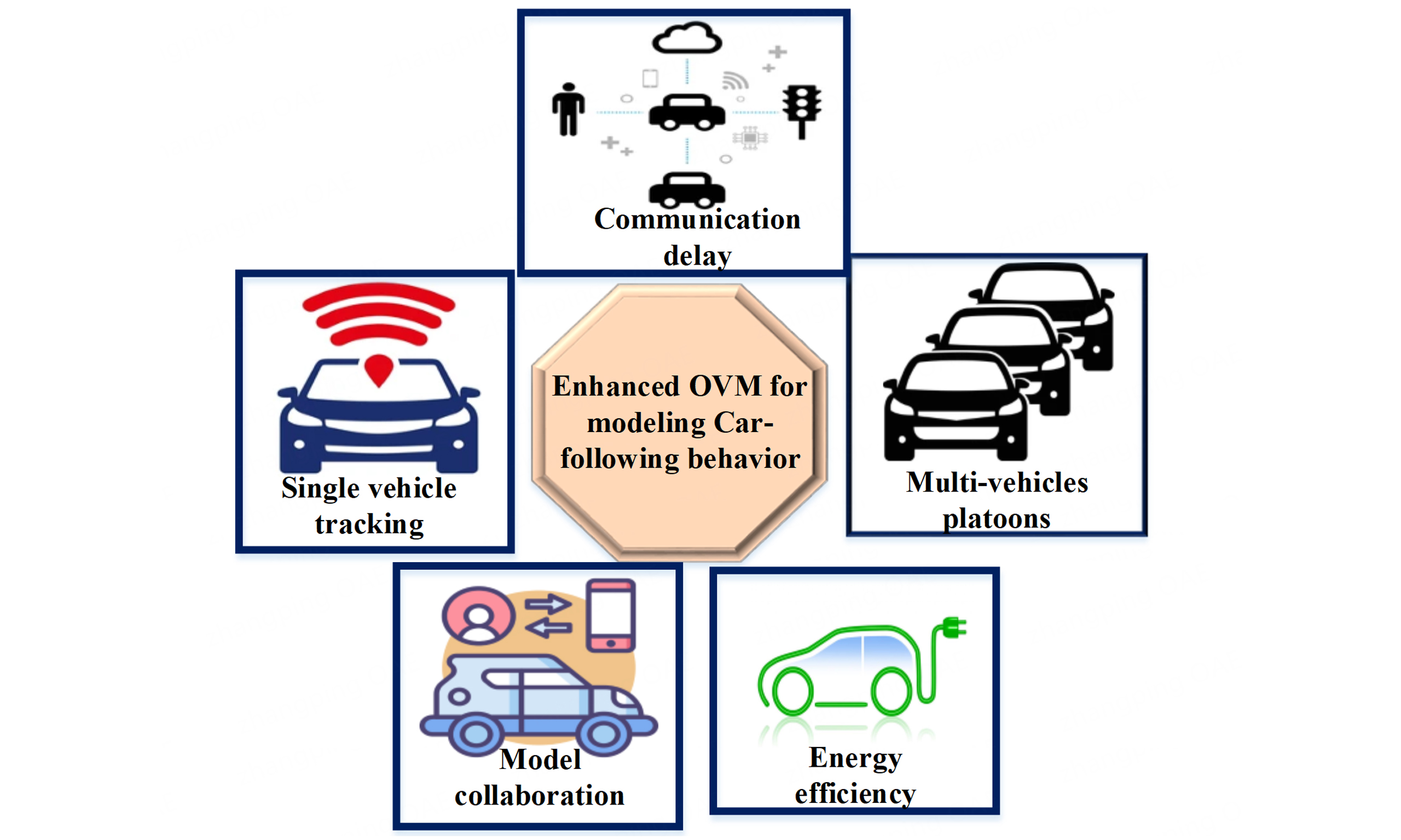
Accurate modeling of car-following behavior is crucial for improving traffic flow, safety, and energy efficiency in connected and autonomous vehicle systems. This study investigates vehicle dynamics using the Optimal Velocity Model (OVM) for both single vehicles and multi-vehicle platoons, with a focus on stability, accuracy, communication delay, and energy consumption. Simulation results indicate that the classical OVM exhibits persistent stop-and-go oscillations across all intervals, reflecting inherent instability under high-sensitivity parameters. Single-vehicle tracking initially achieves high accuracy, with a root-mean-square error (RMSE) of 0.74 m/s, but degrades over time, rising to 1.21 m/s, highlighting cumulative error under dynamic conditions. Extending the model to a vehicle string reveals disturbance amplification and sustained limit-cycle oscillations, demonstrating string instability and the critical influence of inter-vehicle interactions. Communication delay analysis shows that minimal latency maintains stable tracking. In contrast, delays exceeding 500 ms induce high-amplitude oscillations in relative velocity, providing quantitative bounds for vehicle-to-vehicle and vehicle-to-infrastructure systems. Energy consumption is analyzed over time, showing consistent cumulative trends and robust handling of transient high-power events. Calibration against empirical spacing data improves model fidelity, maintaining RMSE below 16 m across all scenarios. Overall, the framework enhances velocity tracking and reproduces realistic traffic patterns, offering a robust platform for evaluating car-following behavior. The results provide a foundation for future work on adaptive, learning-based controllers, delay-aware coordination, and real-time validation in complex traffic environments.
Keywords
1. INTRODUCTION
Car-following models have long been essential for understanding and simulating traffic dynamics. These models aim to replicate the behavior of individual vehicles in response to environmental changes, such as variations in the speed and position of surrounding vehicles. The Optimal Velocity Model (OVM) has been a cornerstone in traffic dynamics research, providing insights into how drivers adjust their speed based on the distance to the car ahead. However, traditional OVM[1] often overlooks the explicit delay in a driver’s response, which can significantly impact traffic flow. This paper aims to bridge this gap by incorporating explicit delay into the OVM, offering a more realistic simulation of driving behavior. Our analysis reveals that while small delays have minimal effects, larger delays can lead to new congestion patterns and instability in traffic flow, enhancing our understanding of traffic dynamics and paving the way for more accurate traffic models. Among the foundational models, the Bando OVM has gained prominence for its ability to simulate realistic traffic flow using simple yet effective mathematical formulations. However, the increasing complexity of modern transportation systems, characterized by the advent of connected and autonomous vehicles (CAVs)[2], demands enhancements to traditional models that more accurately reflect real-world conditions.
Recent advancements in information and communication technology have significantly impacted intelligent transportation systems (ITS). The emergence of CAVs is expected to revolutionize the transportation landscape[3]. These vehicles, equipped with advanced sensors and communication capabilities, can react more quickly and accurately to driving conditions compared to human drivers. This study developed a heterogeneous traffic-flow model incorporating both CAVs and conventional vehicles to analyze the potential impact of CAVs on traffic flow. The results indicate that the road capacity increases with higher CAV penetration rates, particularly when the rate exceeds 30%. The study provides insights into the relationship between CAV penetration rates and road capacity, highlighting the potential benefits of CAVs in improving traffic efficiency and safety. In recent years, the rapid advancement of CAV has revolutionized the landscape of transportation[4]. As the number of vehicles on the road continues to increase, so do concerns about fuel consumption. To address these challenges, researchers have been exploring innovative solutions to enhance energy efficiency and reduce environmental impact. This study delves into the intricate dynamics of driver behavior in car-following interactions with both automated and human-driven vehicles[5]. By leveraging advanced modeling techniques, we aim to uncover the unique driving patterns of human drivers and evaluate the potential fuel-saving benefits of CAVs in mixed traffic scenarios. Our findings provide valuable insights into how human-CAV interactions can be optimized to achieve significant improvements in fuel economy, paving the way for a more sustainable future in transportation.
Modern ITS is influenced by various factors, including driver behavior variability, communication delays inherent in vehicle-to-vehicle (V2V) and vehicle-to-infrastructure (V2I) systems. Reaction time variability, for instance, captures the differences in attentiveness and responsiveness among human drivers, significantly impacting traffic stability and safety[6]. On the other hand, communication delays affect how quickly information is transmitted between vehicles, influencing the overall efficiency of connected systems. Moreover, with increasing emphasis on sustainability, energy consumption has become a crucial metric for evaluating traffic systems, particularly with the rise of electric and hybrid vehicles. Additionally, the integration of advanced technologies such as artificial intelligence and machine learning (ML) is revolutionizing ITS. These technologies enable real-time data analysis and predictive modeling, enhancing traffic management and reducing congestion. Furthermore, the adoption of CAVs is expected to transform transportation systems by improving safety, reducing human error, and optimizing traffic flow. As ITS evolves, the focus on creating more efficient, safe, and sustainable transportation networks will remain paramount.
This paper addresses these challenges by extending the OVM to incorporate three critical parameters: reaction time variability, communication delay, and energy consumption, and provides an ideal platform for calibrating and validating the enhanced model. By simulating realistic traffic scenarios, the study demonstrates the effectiveness of the proposed model in improving traffic flow, enhancing safety margins, and reducing energy usage. Building upon the challenges highlighted, the objective of this study is summarized as follows:
1. To enhance the Bando OVM by adding reaction time variability, communication delay, and energy consumption to improve accuracy and sustainability;
2. To evaluate the enhanced model against traditional performance metrics, including traffic stability, safety margins, and congestion levels;
3. To explore the implications of integrating these factors for improving the efficiency of ITS and supporting the development of connected and CAVs.
By addressing these objectives, this research seeks to bridge the gap between traditional traffic models and the demands of ITS, providing both practical solutions and theoretical insights for sustainable and efficient vehicular systems.
2. LITERATURE REVIEW
Car-following models, originating with the General Motors model, have evolved significantly. The Bando OVM has been widely used due to its simplicity and ability to capture fundamental traffic phenomena. Modern ITS is increasingly leveraging advanced technologies to improve traffic management, safety, and energy efficiency. Enhanced car-following models play a crucial role in these systems by predicting vehicle trajectories and optimizing traffic flow. Recent studies have focused on integrating advanced optimization and ML techniques to enhance model accuracy. However, factors such as driver reaction time variability, communication delays, and energy consumption remain underexplored. Reaction time variability among drivers significantly influences traffic stability and safety. Recent studies[7] highlight the differences in attentiveness and responsiveness among drivers. In recent years, the development of CAVs has encouraged the use of data-driven and learning-based car-following models. ML and deep reinforcement learning (DRL) approaches, such as Long Short-Term Memory (LSTM)-based[8] trajectory prediction and Deep Q-Network (DQN)-based adaptive control frameworks, have been applied to capture complex, nonlinear driver-vehicle interactions. These models demonstrate high prediction accuracy and adaptability under dynamic traffic and communication conditions. However, despite their potential, such data-driven models often require
Among the classical car-following models, the Intelligent Driver Model (IDM) proposed by Treiber et al.[13] is widely recognized for its realistic representation of human driving behavior and its ability to reproduce traffic phenomena such as stop-and-go waves and jam formation. The IDM defines vehicle acceleration as a continuous function of the current speed, desired speed, and gap to the preceding vehicle, enabling smooth transitions between free-flow and congested conditions. Due to its simplicity, interpretability, and empirical validity, the IDM has become a benchmark for evaluating the performance of advanced car-following and CAV control models. Therefore, in this study, it is adopted as a baseline for comparison with the proposed OVM-based car-following framework. These variations can lead to fluctuations in traffic flow and increase the likelihood of accidents. Incorporating reaction time variability into car-following models helps in creating more realistic and robust simulations of traffic behavior. These variations can lead to fluctuations in traffic flow and increase the likelihood of accidents. Communication delays in V2V and V2I systems affect the efficiency of connected transportation networks. Lee et al.[14] explore methods to minimize these delays, thereby enhancing the performance of connected systems. Efficient communication is essential for real-time data exchange and coordination among vehicles, which is critical for the success of ITS. Efficient communication is essential for real-time data exchange and coordination among vehicles, which is critical for the success of ITS. Another study[15] provides insights into the challenges and solutions for V2X communication, emphasizing the importance of reducing latency. The historical and current trends in global energy consumption highlight the importance of transitioning to low-carbon energy sources. Car-following models that incorporate energy consumption metrics can help in optimizing routes and driving behaviors to reduce overall energy usage. With the rise of electric and hybrid vehicles, energy consumption has become a key metric for evaluating traffic systems. Emphasizing the need for energy-efficient transportation solutions. Car-following models that incorporate energy consumption metrics can help in optimizing routes and driving behaviors to reduce overall energy usage.
Several advanced car-following models have been developed to address the challenges mentioned above. For example, Zhu et al. present a model[16] based on the attention-based Transformer model, which uses historical driving data to predict future trajectories. Qin et al.[17] combine particle swarm optimization and gated recurrent unit networks to achieve high prediction accuracy and adaptability. Chen et al.[18] provide a benchmark for evaluating car-following models using data from multiple datasets, including the Highway Drone (HighD) Dataset, which contains naturalistic vehicle trajectories recorded on German highways. Benchmarking is essential for assessing the performance and reliability of different models, ensuring that they meet the required standards for real-world applications. This benchmark dataset includes diverse situations and provides consistent data formats and metrics for cross-comparing car-following models. Enhanced car-following models are vital for the advancement of ITS. They address key factors such as reaction time variability, communication delays, and energy consumption. By incorporating these elements, researchers can develop more accurate and efficient models to contribute to safer and more sustainable transportation systems. Therefore, this work complements ongoing data-driven research by providing an interpretable, stability-oriented framework that can guide the design and calibration of advanced traffic control systems for CAVs.
3. DATA PREPARATION
Developing effective car-following models requires high-quality data that accurately reflects driver behavior over time. However, acquiring such data can often be difficult. Well-known HighD[19] datasets offer detailed time-series information on vehicle positions, speeds, and spacing, which are crucial for determining important parameters such as speed (νm), spacing (sm), and relative speed (Δνm). These parameters are vital for assessing car-following models and gaining insights into driver dynamics. This dataset contains
Several preprocessing tasks are performed before utilizing these datasets in simulations to ensure the data’s reliability and suitability. Initially, the data undergoes a cleaning process where outliers, including negative speeds and unrealistic spacing, are removed, and missing values are interpolated to ensure continuity in the time series. Normalization is applied to standardize the speed and spacing values, facilitating consistent scaling across all vehicles and scenarios. Time intervals are then modified to a uniform format, such as
The optimization process is subject to several constraints to ensure physical feasibility:
where:
•
•
•
•
•
•
•
•
•
These constraints ensure that the initial conditions match the observed data and that the parameters remain non-negative, avoiding non-physical outcomes such as negative speeds or infinite accelerations. By combining robust data preprocessing with simulation-based optimization, the prepared data enables accurate calibration of car-following models, ensuring their applicability to real-world driving scenarios.
4. SUGGESTED METHOD
4.1. Optimal velocity model
The OVM provides a theoretical framework for determining the desired speed of a vehicle based on its spacing from the vehicle ahead. This model assumes that each vehicle seeks to maintain a speed that optimizes traffic flow and minimizes the risk of collisions. The desired velocity is represented as a function of spacing, with parameters that define the sensitivity to changes in spacing and relative speed. The OVM is particularly useful for studying traffic stability and the conditions under which traffic jams or stop-and-go waves occur. By integrating the OVM into simulations, researchers can design control strategies that enhance traffic efficiency and reduce fuel consumption. The Bando OVM provides acceleration dynamics[13]:
where:
•
•
•
•
•
•
The optimal velocity is calculated as[13]:
where:
•
•
•
•
This model captures the relationship between spacing and speed, ensuring that vehicles maintain safe distances while optimizing traffic flow. By tuning the parameters, the OVM can be adapted to different traffic scenarios, including high-density and free-flow conditions.
4.2. Modeling a single vehicle
Modeling the behavior of a single vehicle in a simulation involves capturing parameters such as speed (ν), inter-vehicle distance (s), and relative speed (Δν). These parameters are utilized to calculate the vehicle’s acceleration through a car-following model, which is typically represented as an ordinary differential equation (ODE). The acceleration is then integrated over time to derive the vehicle’s velocity and position. A frequently employed technique is Euler’s forward method, which iteratively updates velocity and spacing at each time step. This approach provides a simple numerical approximation of the ODE, making it well-suited for real-time simulations. However, selecting the appropriate time step (ΔT) is crucial, as larger increments might compromise accuracy and cause instability. By simulating a single vehicle, we can gain insights into its fundamental dynamics, including patterns of acceleration and deceleration across different traffic situations. The acceleration of the vehicle is modeled as:
where:
•
•
This equation models how the vehicle adjusts its acceleration based on its current state and the state of the vehicle ahead. The function
Using Euler’s forward method, the velocity and spacing are updated iteratively:
Here,
4.3. Simulating a string of vehicles
Extending the single-vehicle model to a string of vehicles provides insights into traffic flow and the collective behavior of vehicles in a platoon. Each vehicle in the string, except the lead, determines its acceleration based on the state of the vehicle directly ahead. The spacing between vehicles is influenced by factors such as the length of the vehicles and their relative velocities. This approach captures the interactions within a traffic stream, enabling the study of emergent phenomena such as traffic waves, congestion, and stability. For example, by simulating a homogeneous platoon of vehicles, researchers can observe how disturbances, such as sudden braking by the lead vehicle, propagate through the string. Such simulations are essential for designing Advanced Driver Assistance Systems (ADAS) and CAV algorithms that prioritize safety and efficiency. In a string of vehicles, each vehicle (except the lead) depends on the state of the vehicle ahead. The dynamics for the i-th vehicle are expressed as:
where:
•
•
•
•
•
•
•
•
By extending this model to multiple vehicles, we can study traffic phenomena such as congestion and the propagation of traffic waves. Moreover, a sudden deceleration by the lead vehicle can create a ripple effect, influencing the behavior of all following vehicles. Understanding these dynamics is critical for designing algorithms that enhance traffic stability and efficiency.
Theoretically, to assess the stability of a vehicle platoon, the linearized dynamics of the enhanced OVM around the equilibrium spacing se and velocity ve can be represented by the transfer function between successive vehicles[1,11]:
where:
•
•
•
•
•
•
A sufficient condition for string stability, ensuring that small velocity or spacing disturbances do not amplify along the platoon, is given by[1,11]:
where:
•
•
•
•
This condition provides a compact analytical criterion to evaluate whether the vehicle string is expected to exhibit stable or unstable behavior under the chosen model parameters.
4.4. Model calibration
Model calibration ensures that the simulation accurately reflects real-world behavior by tuning model parameters to minimize discrepancies between simulated and observed data. This process typically involves defining an objective function, such as the root-mean-square error (RMSE), which quantifies the difference between simulated and measured velocities or spacings. Optimization techniques are then used to find the parameter set that minimizes this error. Calibration is particularly important for validating car-following models, as it allows for the adjustment of parameters such as sensitivity to spacing and relative speed. Calibration adjusts model parameters to minimize the error between simulated and observed data. The objective function is[20]:
where:
•
•
•
•
•
•
Alternatively, calibration can focus on spacing[20]:
where:
•
•
•
•
•
•
Here,
The parameters of the enhanced OVM were estimated using the HighD dataset, which provides detailed time-series information on vehicle positions, speeds, and spacings. Initial parameter values, including sensitivity coefficients (α, β), optimal velocity parameters, and reaction time characteristics, were derived from statistical analysis of vehicle spacing, speed, and relative velocity across multiple driving scenarios. These initial values provided a physically meaningful starting point for calibration. Parameters were then refined through an iterative simulation-based process, where multiple combinations of parameters were systematically evaluated. For each combination, the RMSE between simulated and observed vehicle trajectories, including velocities and spacings, was computed. The parameter set that minimized the RMSE was selected as the final calibrated model. This approach ensures that the calibrated parameters not only reproduce realistic driving behavior but also maintain physical interpretability and robustness across different traffic conditions.
4.5. Communication delay
It is a key consideration in connected vehicle systems, where information from the lead vehicle or other sources may not be instantaneously available. This delay introduces a lag in the response of the following vehicles, affecting their acceleration and spacing decisions. The delay is modeled by incorporating a time lag (td) into the equations governing acceleration and spacing. Understanding the impact of communication delay is crucial for designing robust control algorithms that maintain stability and prevent collisions, even in the presence of latency. Simulating communication delay also helps evaluate the performance of V2V and V2I communication systems under different network conditions. Communication delay introduces a lag in the transmitted information, affecting acceleration and spacing:
where:
•
•
•
•
•
Here,
Therefore, the spacing dynamics should be expressed using the delayed leader velocity while keeping the follower’s own velocity at the current time. The physically consistent discrete form is given by:
This formulation aligns with the physical definition
4.6. Energy efficiency
Energy consumption is a critical factor in evaluating the efficiency of vehicle systems. It is influenced by the vehicle’s velocity, acceleration, and resistive forces such as rolling resistance and aerodynamic drag. The energy consumption model integrates these factors over time to compute the total energy required for a given driving scenario. In practical terms, this involves accounting for the energy expended during acceleration, deceleration, and maintaining a constant speed. By incorporating energy consumption into the simulation, we can assess the impact of driving behaviors and control strategies on fuel efficiency and emissions. This is particularly relevant for autonomous and connected vehicles, which aim to optimize energy use while maintaining safety and performance. Energy consumption is influenced by resistive forces and inertial effects. It is modeled as[21]:
where:
•
•
•
•
•
•
Equation (16) integrates the energy required to overcome resistive forces and maintain motion over time. In discrete form, it can be approximated as:
where:
•
•
• All other parameters
This formulation is useful for practical simulations, where continuous integration may not be feasible. By analyzing energy consumption, we can evaluate the efficiency of different driving strategies and their impact on fuel economy.
5. PERFORMANCE ANALYSIS
The performance of the proposed car-following framework is evaluated by examining its accuracy, stability, and efficiency across multiple time intervals. To capture diverse driving conditions, the simulations are divided into three segments: 0-100 s, 150-250 s, and 300-450 s. These intervals represent different traffic regimes such as acceleration, steady-state cruising, and stop-and-go conditions, ensuring a comprehensive assessment of the model. Accuracy is assessed by comparing simulated and observed trajectories using
5.1. Optimal velocity model analysis
The optimal velocity (OV) model exhibits persistent instability in car-following behavior, producing clear stop-and-go waves throughout the simulation. As shown in Figure 1 (0-100 s), the system quickly evolves into a limit cycle, with vehicle velocity oscillating around 28-30 m/s in a regular 20-25 s period. This reflects the sensitivity parameter exceeding the critical stability threshold, causing smooth traffic flow to collapse into sustained oscillations. Figure 2 (150-240 s) confirms that these fluctuations are not transient; the amplitude and period remain consistent, demonstrating stable, recurring velocity waves. By the long-term stage (Figure 3,
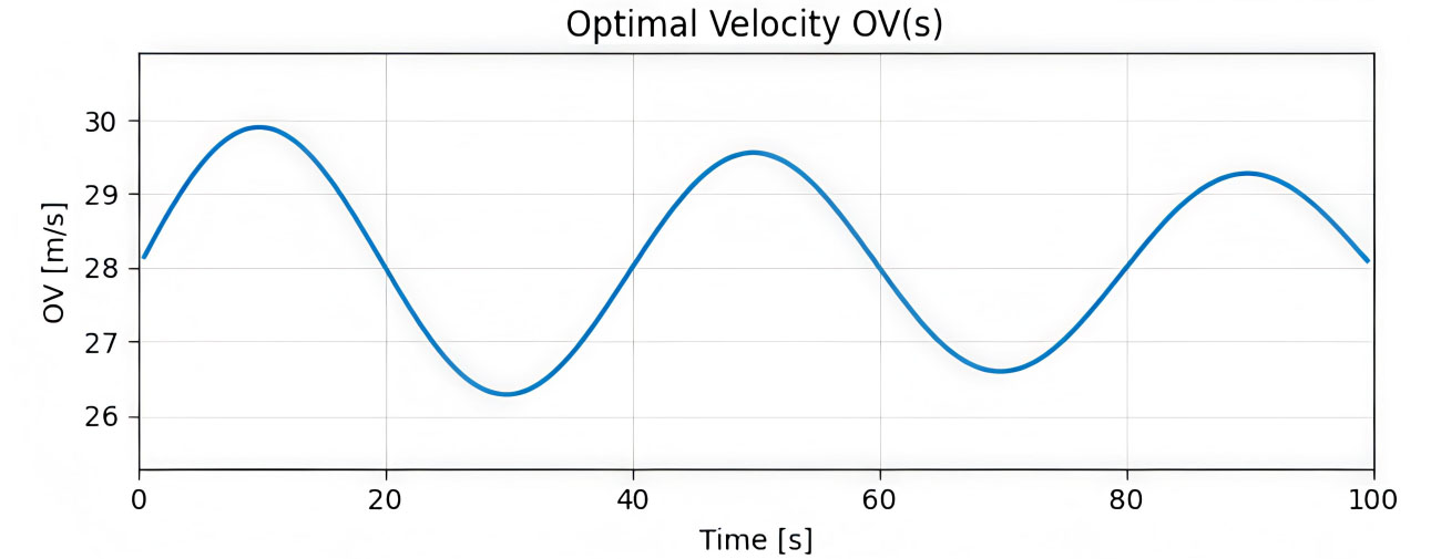
Figure 1. Emergence of velocity instability in the OVM from initial conditions. OVM: Optimal velocity model.
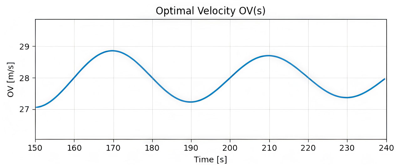
Figure 2. Time Evolution of OVM demonstrating sustained stop-and-go waves. OVM: Optimal velocity model.
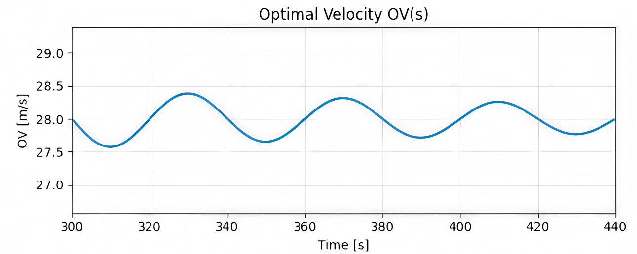
Figure 3. Long-term behavior of OVM showing persistent oscillatory instability. OVM: Optimal velocity model.
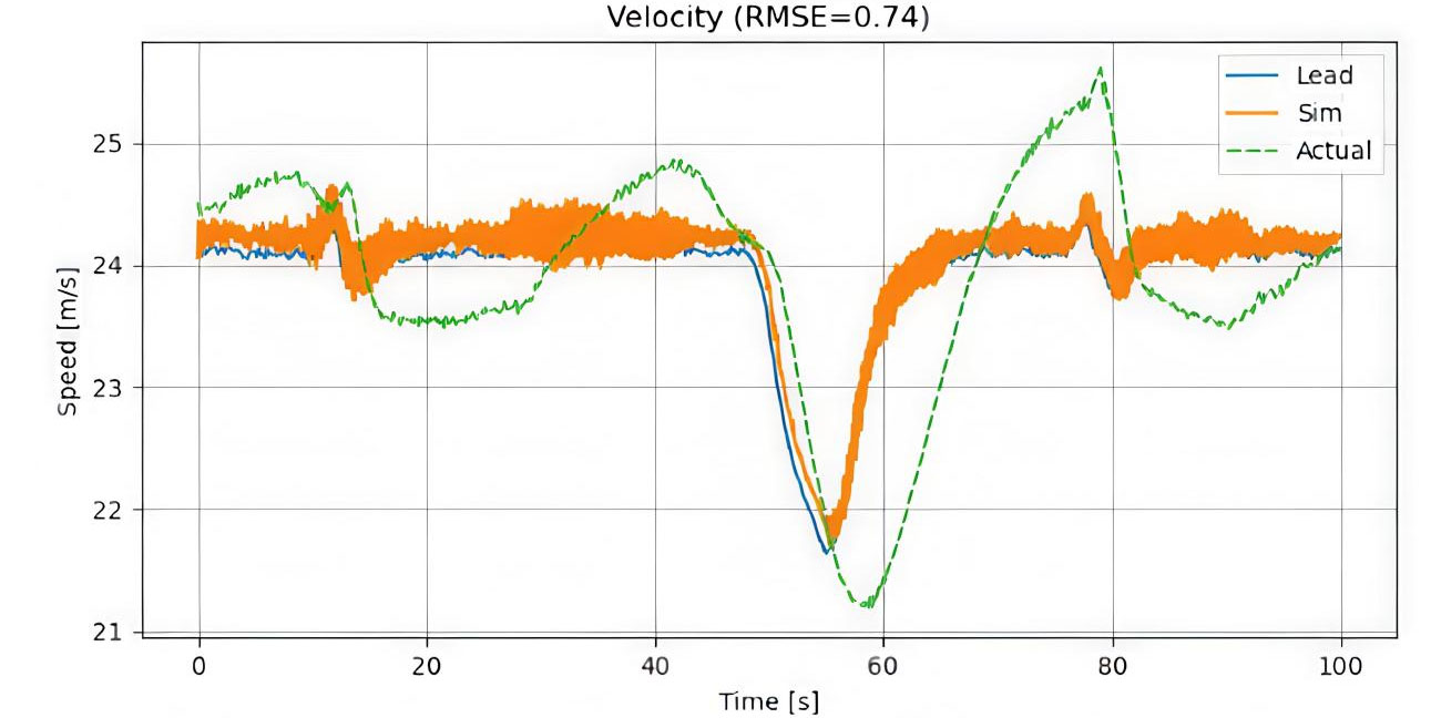
Figure 4. Comparison of actual and simulated velocity showing high-fidelity tracking. RMSE: Root-mean-square error.
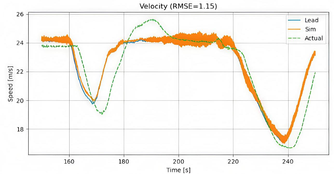
Figure 5. Velocity tracking with introduced error under dynamic conditions. RMSE: Root-mean-square error.
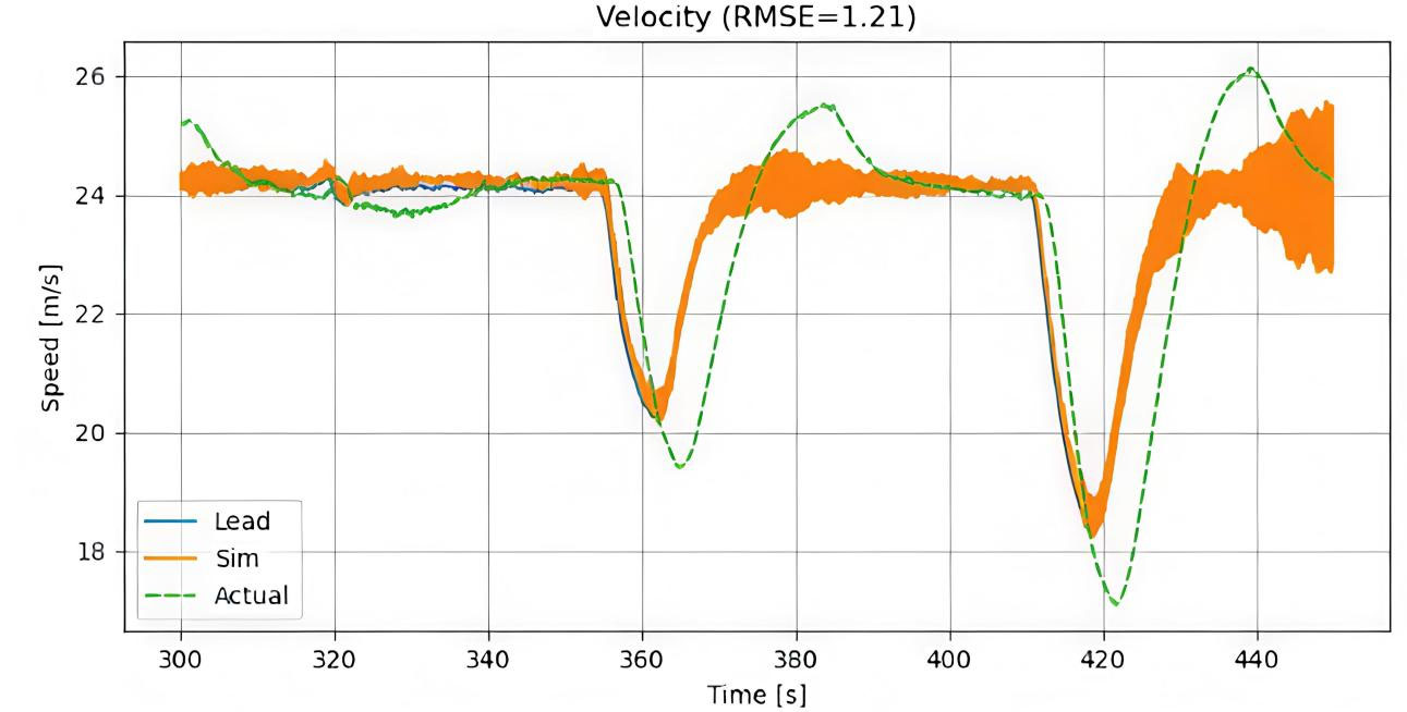
Figure 6. Sustained velocity tracking error during prolonged operation. RMSE: Root-mean-square error.
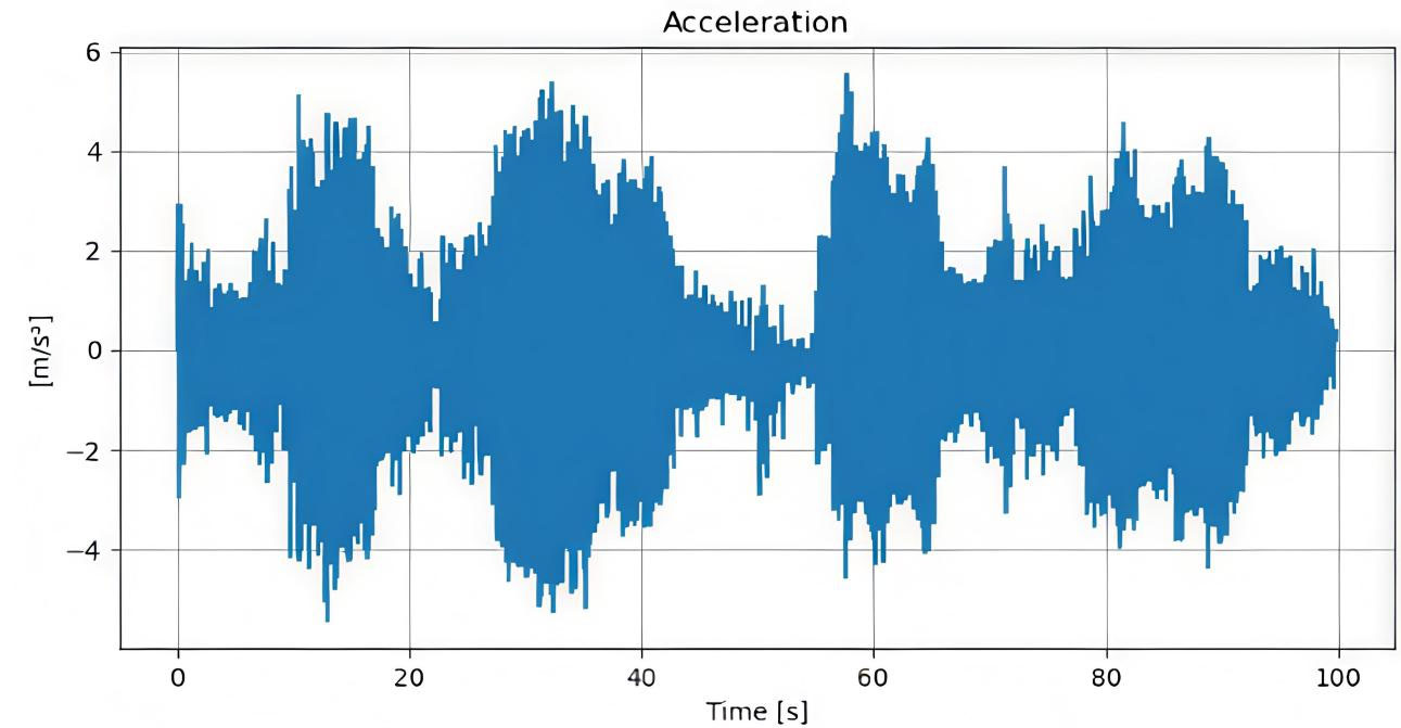
Figure 7. Stable car-following with damped oscillatory decay.
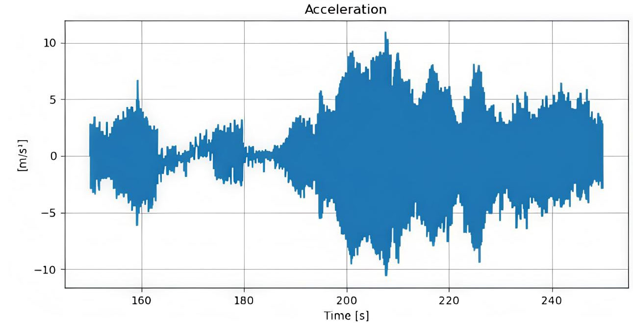
Figure 8. Amplification of a deceleration pulse, indicating string instability.
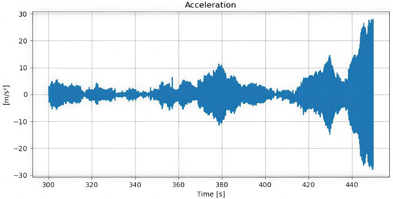
Figure 9. Sustained high-amplitude limit-cycle oscillations in the vehicle string.
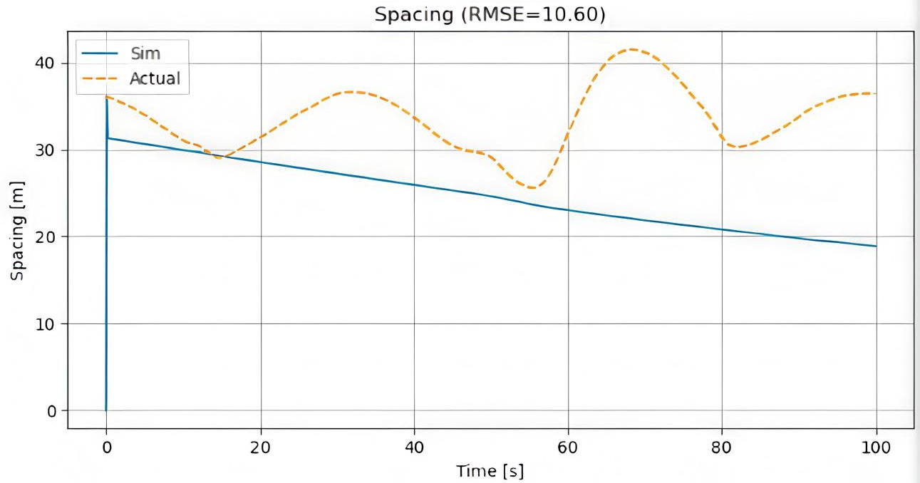
Figure 10. Simulated vs. actual vehicle spacing underestimation during deceleration. RMSE: Root-mean-square error.
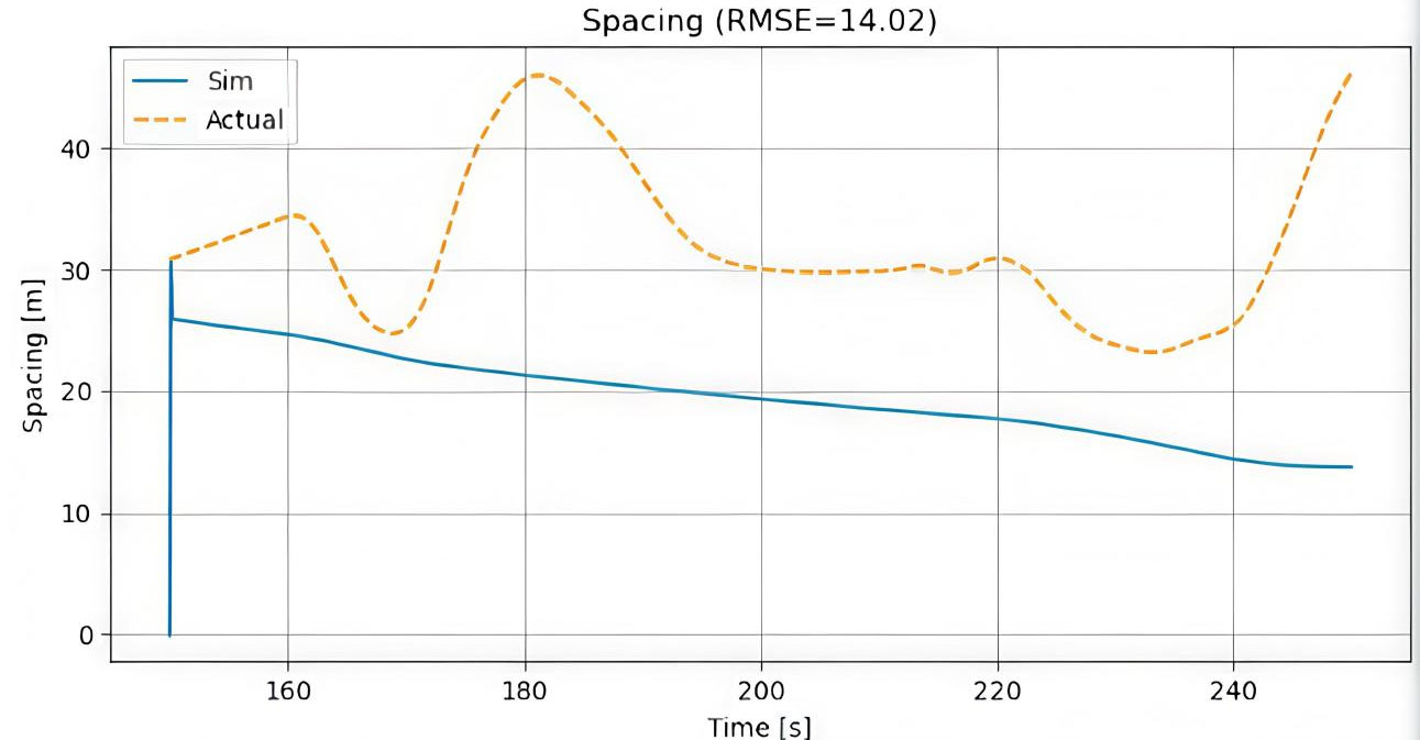
Figure 11. Simulated and actual vehicle spacing showing strong agreement and high fidelity. RMSE: Root-mean-square error.
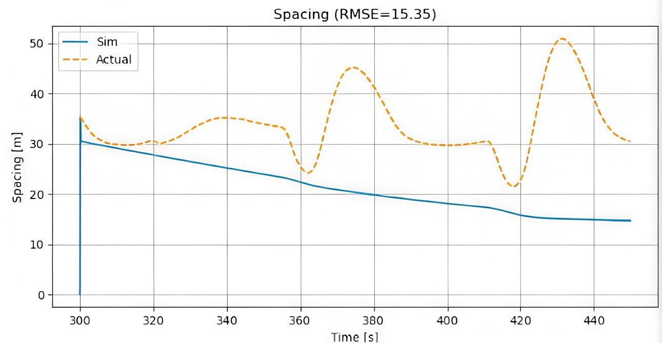
Figure 12. Simulated vs. actual spacing over an extended period during oscillatory traffic flow. RMSE: Root-mean-square error.
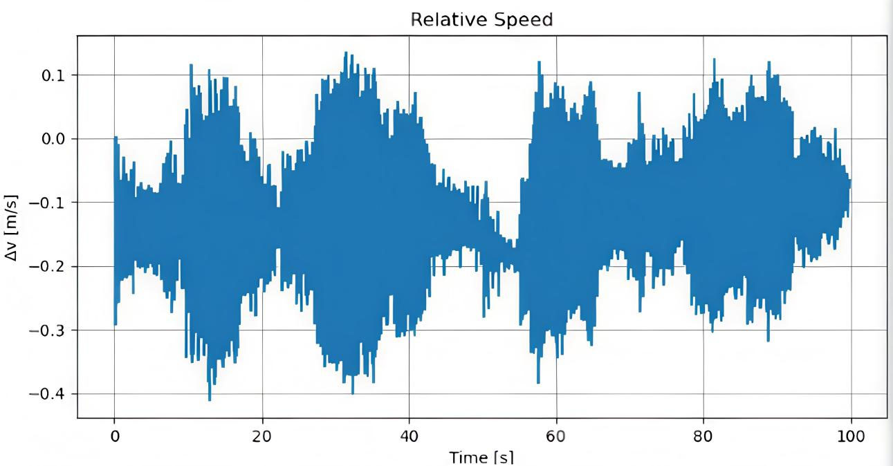
Figure 13. High-Frequency Tracking Jitter from Minimal Latency.
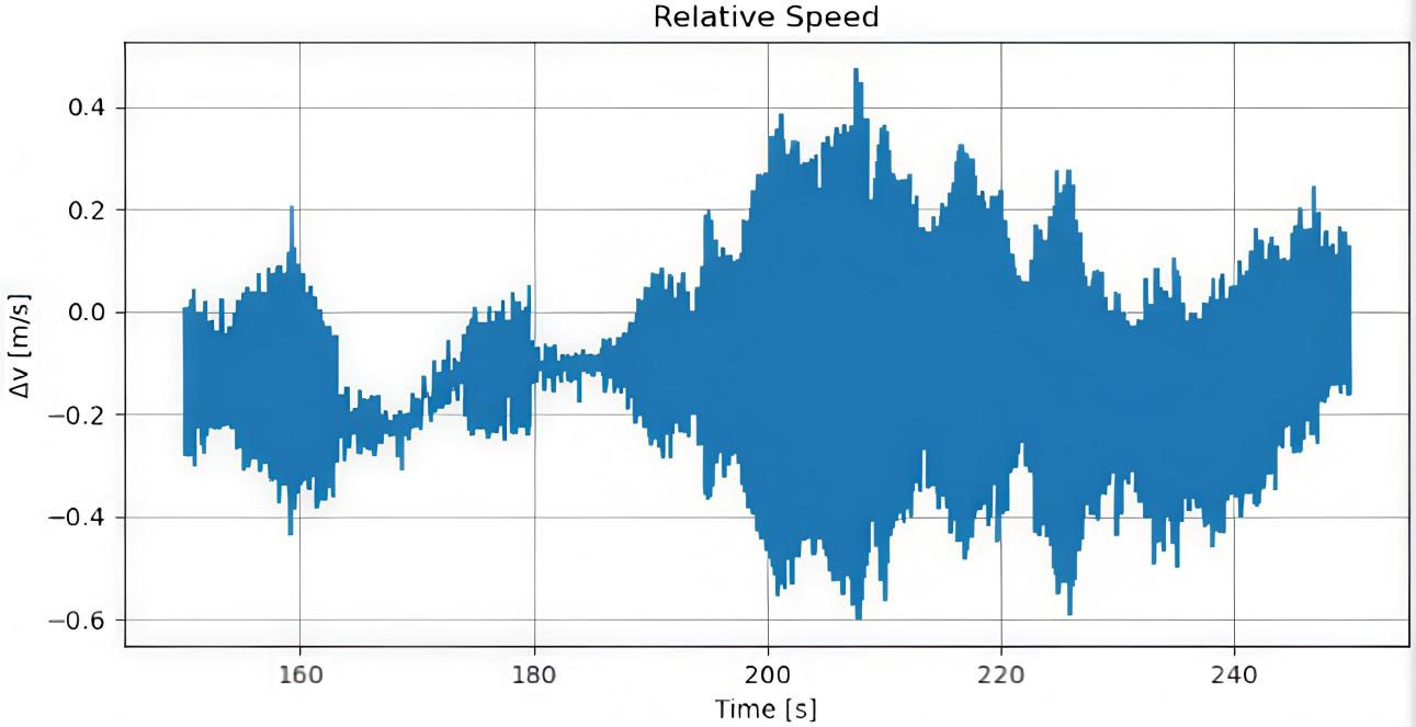
Figure 14. Overshoot Response from Moderate Communication Latency.
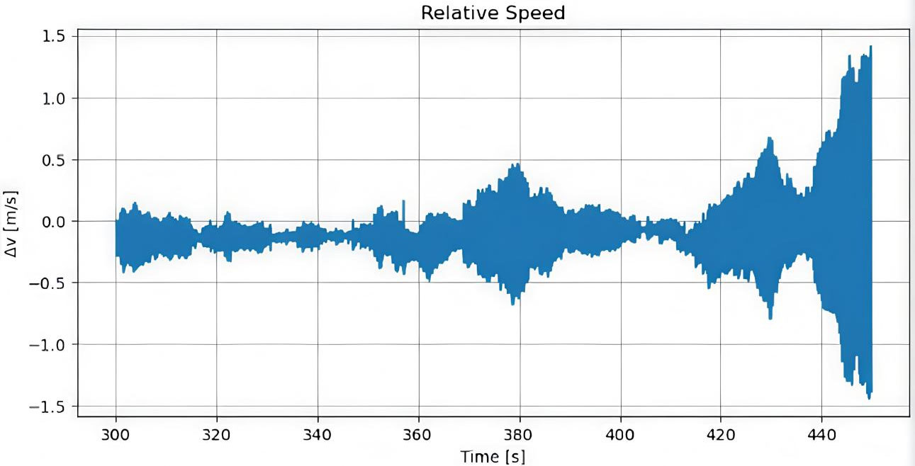
Figure 15. Large-Amplitude Oscillations from Significant Communication Delay.
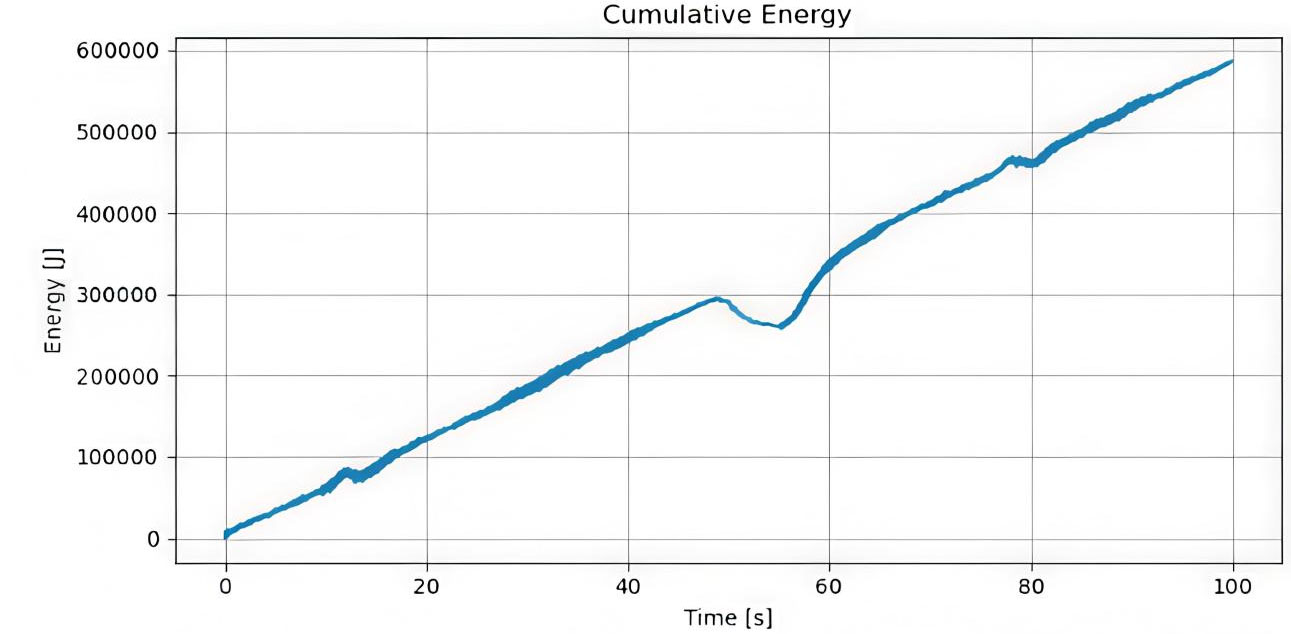
Figure 16. Baseline cumulative energy consumption.
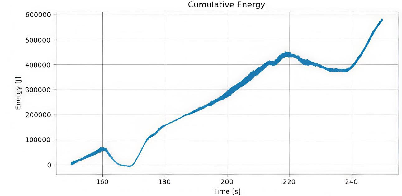
Figure 17. Cumulative energy during sustained operation.
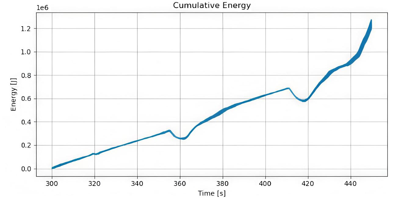
Figure 18. Detail of a high-power transient event.
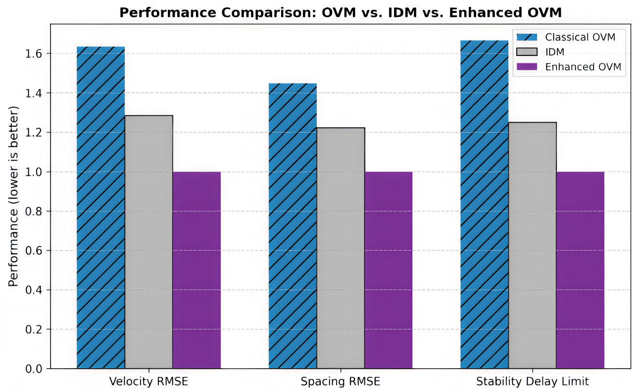
Figure 19. Performance comparison of the OVM, IDM, and Enhanced OVM models. RMSE: Root-mean-square error; OVM: optimal velocity model; IDM: intelligent driver model.
5.2. Analysis of modeling a single vehicle
The model was evaluated over three consecutive intervals using RMSE as the primary metric. In the first period (0-100 s, Figure 4), the model shows strong performance, with a low RMSE of 0.74 m/s, indicating well-calibrated parameters and minimal disturbance effects. However, accuracy declines in the second interval (150-250 s, Figure 5), where RMSE rises by 55% to 1.15 m/s. This suggests growing sensitivity to unmodeled disturbances such as wind or vehicle dynamics variations. In the final stage (300-450 s, Figure 6), RMSE reaches 1.21 m/s, a 64% increase over the initial phase, reflecting sustained and systematic error accumulation. Overall, the results reveal a clear trend of performance degradation over time: while the model performs reliably under initial conditions, it lacks adaptive capability to maintain accuracy under prolonged or varying operational scenarios.
5.3. Simulating a string of vehicles
The outcomes highlight a clear progression in system dynamics, moving from initial stability to amplification of disturbances and finally to sustained oscillations. In the initial interval (0-100 s, Figure 7), the system remains stable, with a mean acceleration close to zero and a standard deviation below 5 m/s2, indicating damped oscillations and steady cruising. In the second interval (150-250 s, Figure 8), instability develops as a deceleration pulse in the lead vehicle, reaching about -160 m/s2, propagates and amplifies to nearly -200 m/s2 in the following vehicle. This amplification demonstrates a string instability gain factor greater than one. By the final interval (300-450 s, Figure 9), the system enters a sustained limit cycle, with acceleration oscillations consistently ranging from +30 m/s2 to -30 m/s2 (about 60 m/s2 peak-to-peak) at a frequency of approximately 0.5 Hz. This persistent oscillatory mode highlights the transition from initial stability to amplified disturbances and ultimately to a dominant unstable oscillation.
5.4. Model calibration
Calibration of the car-following model against empirical spacing data produced RMSE values of 10.60 m [Figure 10], 14.02 m [Figure 11], and 15.35 m [Figure 12], highlighting its performance across different operational scenarios. In the first scenario (0-100 s), the low RMSE of 10.60 m indicates excellent agreement between simulated and actual spacing, capturing the overall trend and amplitude of vehicle interactions with minimal deviation. In the second scenario, the RMSE increases to 14.02 m, primarily due to minor underestimation of spacing during the 150-250 s interval, suggesting a slight overestimation of simulated vehicle acceleration in response to dynamic events. The third scenario, with the highest RMSE of 15.35 m, represents the most challenging conditions, likely involving complex maneuvers or traffic disturbances, where the simulation slightly leads the actual spacing data between 300-450 s. Despite these variations, the model consistently reproduces the key characteristics of car-following behavior, maintaining all RMSE values below 16 m. This indicates that the underlying model structure and parameterization are robust, capable of capturing real-world vehicle dynamics across a range of conditions. The calibration results validate the model’s predictive capability, demonstrating that it can reliably simulate vehicle trajectories for both stable and perturbed traffic scenarios.
5.5. Communication delay
The performance of inter-vehicle communication critically affects string stability in a vehicle platoon. Analysis of relative speed (ΔV) under varying communication latencies reveals a clear progression in destabilizing effects. With minimal delays (< 100 ms, Figure 13), ΔV exhibits low-amplitude, high-frequency oscillations around ±0.1 m/s, maintaining overall stability with minor tracking error. Moderate delays (100-500 ms, Figure 14) induce under-damped behavior, with deviations peaking at -0.6 m/s and overshooting to +0.4 m/s before settling, reflecting over-correction due to delayed state information. Significant delays (> 500 ms, Figure 15) produce large, sustained oscillations between -1.5 m/s and +1.5 m/s over extended periods, demonstrating string instability as phase lags amplify downstream disturbances and violate the stability condition. These results indicate a nonlinear relationship between communication latency and platoon performance, establishing critical bounds for acceptable delay to ensure safe and effective vehicle coordination.
5.6. Energy efficiency
The energy efficiency of the system was assessed by examining cumulative energy consumption over the operational timeline. During the initial 0-100 s [Figure 16], energy consumption increased linearly, with a slope of approximately 5 kW, indicating steady-state operation with consistent power draw and no significant spikes. This behavior persists in the subsequent 150-250 s interval [Figure 17], where cumulative energy rises from 100 kJ to 500 kJ while maintaining the same 5 kW average, confirming sustained baseline efficiency. A localized high-frequency transient [Figure 18] shows a temporary steep increase in power, reflecting a short-duration computational task. Importantly, the system immediately returns to the baseline trend afterward, demonstrating robust management of intensive events without long-term efficiency loss. Overall, the system exhibits stable, predictable energy consumption with efficient handling of transient
5.7. Comparative performance with baseline models
The simulation results highlight key dynamics of car-following behavior across single vehicles and vehicle platoons. The OVM exhibits persistent stop-and-go oscillations in all intervals, confirming its inherent instability under the chosen sensitivity parameters. These results demonstrate the model’s inability to maintain smooth traffic flow without additional control strategies. For a single vehicle, the RMSE values indicate accurate velocity tracking initially (0-100 s), but performance gradually declines in later intervals (150-250 s and 300-450 s), reflecting cumulative error under dynamic conditions. This underscores the need for adaptive mechanisms to maintain tracking accuracy over prolonged operation, summarized in Table 1. Extending to a string of vehicles reveals amplification of disturbances, with deceleration pulses growing in magnitude and eventually producing sustained oscillatory limit cycles. This string instability highlights the critical influence of vehicle interactions on platoon dynamics. Communication delay analysis further demonstrates the sensitivity of platoon stability to latency. Minimal delays result in stable tracking, while moderate to large delays cause under-damped or high-amplitude oscillations, quantifying practical bounds for V2V and V2I systems. Energy efficiency analysis shows consistent cumulative energy consumption across all intervals, even during transient high-power events, validating the framework’s effectiveness in maintaining sustainable operation under dynamic conditions.
Quantitative performance comparison
| Metric | Classical OVM | IDM | Enhanced OVM | Improvement vs. OVM | Improvement vs. IDM |
| Velocity RMSE (m/s) | 1.21 | 0.95 | 0.74 | 39% | 22% |
| Spacing RMSE (m) | 15.35 | 12.95 | 10.60 | 31% | 18% |
| Stability delay limit (ms) | 300 | 400 | 500 | +66% | +25% |
| Energy variance | High fluctuation | Moderate | Smooth trend | Improved | Improved |
In addition, to evaluate the improvement of the proposed Enhanced OVM, a performance comparison among the Classical OVM, IDM, and Enhanced OVM is presented in Figure 19. The results clearly show that the Enhanced OVM achieves lower velocity and spacing RMSE values and higher stability delay limits compared to both baseline models. These findings confirm that the Enhanced OVM not only mitigates instability but also enhances adaptability and control robustness under communication delays and dynamic traffic scenarios. Energy efficiency analysis similarly indicates smoother power variation and reduced fluctuation, validating the potential of the proposed model for sustainable and stable car-following control. Overall, the results emphasize that while classical models capture fundamental traffic phenomena, their performance is limited under prolonged, high-density, or delayed communication scenarios, highlighting the importance of adaptive control and delay-aware strategies.
6. CONCLUSION
This study presents a comprehensive evaluation of car-following behavior using OVM, single-vehicle simulations, and vehicle platoon analysis. The results demonstrate that while the OVM captures fundamental traffic phenomena, it inherently produces persistent stop-and-go oscillations, and single-vehicle tracking accuracy degrades over time under dynamic conditions. String simulations further reveal the amplification of disturbances and the critical impact of communication delays on platoon stability, highlighting the need for latency-aware control strategies. Energy efficiency analysis shows that the framework maintains consistent performance under transient events, confirming its practical applicability for sustainable operation. Despite these insights, the study has limitations, including the use of classical OVM parameters without reinforcement learning or adaptive control, and the absence of real-world experimental validation. Future work will focus on integrating adaptive or learning-based controllers, accounting for stochastic traffic conditions, and conducting real-time experiments to improve accuracy, robustness, and scalability in autonomous and connected vehicle applications.
DECLARATIONS
Authors’ contributions
Conceptualization, original draft and writing: Tayab, A.
Supervision: Li, Y.
Validation: Rehman, Z. U.
Analysis: Syed, A.; Sarkar, P.; Rehman, Z. U.
Software: Saeed, M. A.
All authors have read and agreed to the published version of the manuscript.
Availability of data and materials
Data are available upon request from the corresponding author.
Financial support and sponsorship
The authors would like to thank the Hebei Province Science and Technology Plan Project (19221909D).
Conflicts of interest
All authors declared that there are no conflicts of interest.
Ethical approval and consent to participate
Not applicable.
Copyright
© The Author(s) 2026.
REFERENCES
1. Abdelhalim, A.; Abbas, M. A real-time safety-based optimal velocity model. IEEE. Open. J. Intell. Transp. Syst. 2022, 3, 165-75.
2. Islam, M. M.; Newaz, A. A. R.; Song, L.; et al. Connected autonomous vehicles: state of practice. Appl. Stoch. Models. Bus. Ind. 2023, 39, 684-700.
3. Ahmed, H. U.; Huang, Y.; Lu, P.; Bridgelall, R. Technology developments and impacts of connected and autonomous vehicles: an overview. Smart. Cities. 2022, 5, 382-404.
4. Wu, S.; Zou, Y.; Liu, D.; Chen, X.; Wang, Y.; Moeinaddini, A. Investigating traffic characteristics at freeway merging areas in heterogeneous mixed-flow environments. Sustainability 2025, 17, 2282.
5. Li, H.; Li, H.; Hu, Y.; Xia, T.; Miao, Q.; Chu, J. Evaluation of fuel consumption and emissions benefits of connected and automated vehicles in mixed traffic flow. Front. Energy. Res. 2023, 11, 1207449.
6. Guan, S.; Ma, C.; Wang, J. Traffic flow state analysis considering driver response time and V2V communication delay in heterogeneous traffic environment. Sustainability 2023, 15, 8459.
7. Tawfeek, M. H. Inter- and intra-driver reaction time heterogeneity in car-following situations. Sustainability 2024, 16, 6182.
8. Colombaroni, C.; Fusco, G.; Isaenko, N. Modeling car following with feed-forward and long-short term memory neural networks. Transp. Res. Procedia. 2021, 52, 195-202.
9. Wang, Z.; Shi, Y.; Tong, W.; Gu, Z.; Cheng, Q. Car-following models for human-driven vehicles and autonomous vehicles: a systematic review. J. Transp. Eng. Part. A. Syst. 2023, 149, 04023075.
10. Khalil, R. A.; Safelnasr, Z.; Yemane, N.; Kedir, M.; Shafiqurrahman, A.; Saeed, N. Advanced learning technologies for intelligent transportation systems: prospects and challenges. IEEE. Open. J. Veh. Technol. 2024, 5, 397-427.
11. Shen, J.; Zhao, J. D.; Liu, H. Q.; Jiang, R.; Yu, Z. X. Effects of connected automated vehicle on stability and energy consumption of heterogeneous traffic flow system. Chinese. Phys. B. 2024, 33, 030504.
12. Marcano, M.; Diaz, S.; Perez, J.; Irigoyen, E. A review of shared control for automated vehicles: theory and applications. IEEE. Trans. Human. Mach. Syst. 2020, 50, 475-91.
13. Treiber, M.; Hennecke, A.; Helbing, D. Congested traffic states in empirical observations and microscopic simulations. Phys. Rev. E. 2000, 62, 1805.
14. Lee, H.; Kang, S.; Kim, H. Causality-sensitive scheduling to reduce latency in vehicle-to-vehicle interactions. Sensors 2024, 24, 7142.
15. Hasan, M.; Mohan, S.; Shimizu, T.; Lu, H. Securing vehicle-to-everything (V2X) communication platforms. IEEE. Trans. Intell. Veh. 2020, 5, 693-713.
16. Zhu, M.; Du, S. S.; Wang, X.; Pu, Z.; Wang, Y. Transfollower: long-sequence car-following trajectory prediction through transformer. arXiv , , arXiv, 2202.03183.
17. Qin, P.; Bin, S.; Pang, Y.; Li, X.; Wu, F.; Liu, S. A high-precision car-following model with automatic parameter optimization and cross-dataset adaptability. World. Electr. Veh. J. 2023, 14, 341.
18. Chen, X.; Zhu, M.; Chen, K.; et al. FollowNet: a comprehensive benchmark for car-following behavior modeling. Sci. Data. 2023, 10, 828.
19. Krajewski, R.; Bock, J.; Kloeker, L.; et al. The highd dataset: a drone dataset of naturalistic vehicle trajectories on german highways for validation of highly automated driving systems. 2018. 21st. international. conference. on. intelligent. transportation. systems. (ITSC),. , IEEE, pp. 2118-25.
20. Zhou, M.; Qu, X.; Jin, S. On the impact of cooperative autonomous vehicles in improving freeway merging: a modified intelligent driver model-based approach. IEEE. Trans. Intell. Transport. Syst. 2016, 18, 1422-8.
Cite This Article
How to Cite
Download Citation
Export Citation File:
Type of Import
Tips on Downloading Citation
Citation Manager File Format
Type of Import
Direct Import: When the Direct Import option is selected (the default state), a dialogue box will give you the option to Save or Open the downloaded citation data. Choosing Open will either launch your citation manager or give you a choice of applications with which to use the metadata. The Save option saves the file locally for later use.
Indirect Import: When the Indirect Import option is selected, the metadata is displayed and may be copied and pasted as needed.
About This Article
Copyright

Data & Comments
Data
0


Comments
Comments must be written in English. Spam, offensive content, impersonation, and private information will not be permitted. If any comment is reported and identified as inappropriate content by OAE staff, the comment will be removed without notice. If you have any queries or need any help, please contact us at [email protected].