Download PDF
Research Article  |  Open Access  |  22 Jul 2026

Learning-based robust control of modular robot manipulators: an experimental investigation

Views: 15 |  Downloads: 4 |  Cited:  0
Intell. Control Syst. 2026, 1, 3.
10.20517/ics.2026.06 |  © The Author(s) 2026.
Author Information
Article Notes
Cite This Article

Abstract

This paper proposes a learning-based robust control method for modular robot manipulators (MRMs).The dynamic model of MRMs is deployed by using a joint torque estimation method. In contrast to conventional methods, this study tackles the uncertainty inherent in the robot model by accounting not only for friction modeling inaccuracies and interconnection dynamic coupling (IDC), but also for the torque transmission error of the harmonic drive and the measurement deviation. Each of these model uncertainties is individually compensated through a purposefully designed robust neural network controller. The asymptotic stability of the proposed robotic control strategy is rigorously established. A comprehensive series of experiments is carried out to verify the effectiveness and superiority of the presented control approach.
Keywords

Modular robot manipulators, radial basis function neural network, robust control, model uncertainty

INTRODUCTION

With the ongoing evolution of Industry 5.0[1-3] the scope of robotic applications has broadened considerably, encompassing domains such as rehabilitation, motion assistance, and industrial operations. In recent years, modular robot manipulators (MRMs) have garnered significant research attention, owing to their superior structural characteristics and enhanced adaptability relative to conventional robotic manipulators. MRMs consist of joint modules equipped with standardized electromechanical interfaces, which can be configured into diverse assemblies to accommodate varying operational environments and task requirements, without necessitating adjustments to the control parameters of any other subsystem within the robotic platform[4]. By virtue of their flexible configurability and ease of assembly, MRMs are frequently deployed in hazardous and unpredictable settings, including space exploration, disaster response, and extreme-temperature operations[5].

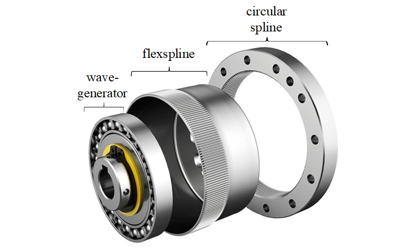
Beyond modularity, lightweight robot manipulators capable of handling substantial payloads have drawn growing interest from both robotic system designers and industrial manufacturers. In[6], a direct-drive, lightweight, and optimized hand exoskeleton prototype was introduced, designed to rest on the dorsal aspect of the hand to keep the palm free for interaction with real or virtual objects. Harmonic drives (HDs) are widely utilized in the development of such manipulators due to their favorable attributes, including high reduction ratios, compact form factors, low weight, and coaxial architecture[7]. A conventional harmonic drive comprises a wave generator, a circular spline, and a flexspline positioned between the two. Over the past several years, substantial efforts have been directed toward the analytical modeling of HDs, with the resulting insights subsequently adopted and refined to address challenges in torque estimation[8,9] and position control[10-13] for HD-based robots. Traditional approaches generally presume that the input angle of the flexspline (corresponding to the gear-toothed circumference) is identical to the output angle of the wave generator (associated with the outer rim of the ball bearing). In practice, however, perfect coaxial alignment between the inner race axis of the wave generator and the flexspline axis is not consistently maintained due to the presence of the ball bearing[14]. As a result, a small angular discrepancy arises between the empirically measured flexspline output and the theoretical prediction - the latter being defined as the wave generator displacement multiplied by the gear ratio. This discrepancy, referred to as kinematic error, can induce localized torque ripple in HD transmission. Nonetheless, neither the kinematic error nor the resulting torque ripple can be measured in real time, and isolating their effects from the overall deformation or torque signal remains a formidable challenge[15]. Therefore, there is a pressing need to develop a comprehensive harmonic drive model that incorporates kinematic inaccuracies and facilitates the effective mitigation of torque ripple.

To mitigate the coupling effect, Liu et al. proposed a distributed control strategy for MRMs equipped with torque sensing[16]. In this framework, each module is furnished with an integrated joint torque sensor, and the corresponding sensor readings are utilized to automatically compensate for the coupling effect. This approach markedly reduces the complexity associated with modular manipulator modeling. Nevertheless, it does not take into account the measurement error within the manipulator system. Since the feedback of such measurement errors into the control loop degrades overall control performance, these errors should be minimized to the greatest extent possible in order to enhance control accuracy.

In robotic systems, the deployment of an appropriate controller constitutes a critical factor in ensuring satisfactory operational performance[17]. To enhance control accuracy, learning-based control methodologies have been introduced. Several representative studies are outlined below. Shen et al. developed a neural-network-based adaptive iterative learning control strategy for strict-feedback nonlinear systems subject to unknown state delays and input saturation[18]. Wang et al. examined the passivity and dissipativity properties of discrete-time fractional generalized delayed Cohen-Grossberg neural networks[19]. Brief [20] investigated the iterative learning control problem for constrained multi-input multi-output nonlinear systems under state alignment conditions with varying trial lengths. The aforementioned works have substantially inspired the present research.

To address this issue, the present paper develops a dynamic model that incorporates not only friction modeling errors and interconnection dynamic coupling (IDC), but also the torque transmission error of the harmonic drive and the measurement deviation. Drawing upon an analysis of model uncertainty, a robust neural network controller is devised for the manipulator. Specifically, the controller compensates for friction modeling errors through robust control, while simultaneously employing a neural network to approximate and compensate for the remaining model uncertainties - comprising the IDC term, the torque transmission deviation of the harmonic drive, and the measurement disturbance - and concurrently suppressing controller chattering. The asymptotic stability of the resulting closed-loop system is rigorously established via Lyapunov theory. Subsequently, a two-degree-of-freedom robotic experimental platform is constructed to validate the effectiveness of the proposed controller.

The main innovations of this article are reflected in the following two aspects:

A Joint torque estimation method based on the harmonic transmission flexibility model is adopted instead of using a joint torque sensor. Moreover, a learning-based robust control method is utilized to handle friction modeling error, interconnection dynamic coupling, and torque transmission error.

Unlike traditional learning control methods based on neural networks, which can only prove the system is uniformly ultimately bounded. The stability proof ensures that the closed-loop system is asymptotically stable, and the proposed method has been verified to be effective through experiments.

DYNAMIC MODELING OF MODULAR ROBOT MANIPULATOR WITH HARMONIC DRIVE

Harmonic drive model

Consider a class of MRMs consisting of $$ n $$ modules. Each self-contained rotary joint module integrates the following components: a direct current (DC) motor serving as the actuator, and two encoders located on the motor side and the link side, respectively, for acquiring the position and velocity information of both the motor and the link. A harmonic drive is employed as a speed reducer. The angular positions at the harmonic drive components, as detailed in [15], can be determined using the ideal input–output kinematic relationship.

$$ \begin{equation} {{\theta }_{wi}}={{\gamma }_{i}}{{\theta }_{fi}} \end{equation} $$

where subscript “$$ i $$” is $$ i $$th module. Denote wave-generator angular position as $$ {{\theta }_{wi}} $$, gear ratio as $$ {{\gamma }_{i}} $$, flexspline output position as $$ {{\theta }_{fi}} $$. Ideal static force equilibrium among components can then express as

$$ \begin{equation} {{\tau }_{wi}}=\frac{1}{{{\gamma }_{i}}}{{\tau }_{fi}} \end{equation} $$

where the variables $$ {{\tau }_{wi}} $$ and $$ {{\tau }_{fi}} $$ signify torque acting on the wave generator as well as the flexspline output torque, respectively. As is customary in the existing literature and standard practice, the circular spline is held stationary, thereby designating the wave generator as the input member and the flexspline as the output. Consequently, the relationship $$ {{\theta }_{ci}}=0 $$ holds, and the torque associated with the fixed circular spline requires no further consideration.

Nevertheless, empirical data characterizing the input–output relationship exhibit a pronounced departure from linearity; specifically, the output does not scale proportionally with the input. Potential sources of this nonlinear behavior include frictional torques, torsional compliance within the harmonic drive components, and kinematic inaccuracies. By first establishing the ideal kinematic constraints that govern motion and force transmission in a harmonic drive, these additional dynamic effects can be systematically incorporated through the introduction of friction, compliance, and kinematic error terms. The resulting compliant response of an MRM joint actuated by a harmonic drive is considered, which references the established compliance model of HD. $$ {{\theta }_{wOi}} $$ and $$ {{\theta }_{wIi}} $$ represent angular positions of wave generator's outer as well as central parts within the joint, while $$ {{\theta }_{fOi}} $$ as well as $$ {{\theta }_{fIi}} $$ mean angular position of flexspline at the load and gear side. The quantity $$ {{\tau }_{mri}} $$ means motor friction, and $$ {{\tau }_{fri}} $$ denotes lumped friction torque of harmonic drive, encompassing bearing friction in the wave generator, friction arising from gear-tooth meshing between the flexspline and circular spline, in addition to output bearing friction, as perceived from the output side of the transmission. Furthermore, $$ {{I}_{mi}} $$ denotes combined inertia of DC motor, while $$ {{k}_{wi}} $$ as well as $$ {{k}_{fi}} $$ are local elastic coefficients for wave generator as well as flexspline.

Upon incorporating frictional losses within harmonic drive transmission, Equation (2) transforms into the following form

$$ \begin{equation} {{\tau }_{wi}}={{\tau }_{i}}-{{\tau }_{mri}}=\frac{1}{{{\gamma }_{i}}}({{\tau }_{fi}}-{{\tau }_{fri}}) \end{equation} $$

where $$ {{\tau }_{i}} $$ is motor torque. Furthermore, the torsional deformations of the flexspline as well as the wave generator can be defined

$$ \begin{equation} \Delta {{\theta }_{fi}}={{\theta }_{fOi}}-{{\theta }_{fIi}} \end{equation} $$

$$ \begin{equation} \Delta {{\theta }_{wi}}={{\theta }_{wOi}}-{{\theta }_{wIi}} \end{equation} $$

It is worth noting from Equations (4) and (5) that only the wave generator input position $$ {{\theta }_{wIi}} $$ (i.e., the motor angle) and the flexible output position $$ {{\theta }_{fOi}} $$ (i.e., the joint angle) can be measured, position measurements are acquired via the motor-side encoder as well as the link-side encoder[21,22]. The harmonic drive’s total torsional angle within the $$ i $$th joint may subsequently be determined from these available positions using the relationship presented below

$$ \begin{equation} \Delta {{\theta }_{i}}={{\theta }_{fOi}}-\frac{{{\theta }_{wIi}}}{{{\gamma }_{i}}} \end{equation} $$

By adding and subtraction $$ {{\theta }_{fIi}} $$ as well as $$ \frac{{{\theta }_{wOi}}}{{{\gamma }_{i}}} $$ in Equation (6), it has

$$ \begin{equation} \begin{aligned} & \Delta {{\theta }_{i}}={{\theta }_{fOi}}-\frac{{{\theta }_{wIi}}}{{{\gamma }_{i}}}\Delta {{\theta }_{i}}={{\theta }_{fOi}}-{{\theta }_{fIi}}+\left( \frac{{{\theta }_{wOi}}}{{{\gamma }_{i}}}-\frac{{{\theta }_{wIi}}}{{{\gamma }_{i}}} \right)+\left( {{\theta }_{fIi}}-\frac{{{\theta }_{wOi}}}{{{\gamma }_{i}}} \right) \\ & =\Delta {{\theta }_{fi}}+\frac{\Delta {{\theta }_{wi}}}{{{\gamma }_{i}}}+\Delta {{\theta }_{upi}} \end{aligned} \end{equation} $$

where $$ \Delta {{\theta }_{upi}} $$ represents kinematic error, defined as difference between measured flexspline output as well as its expected value, and is expressed as

$$ \begin{equation} \Delta {{\theta }_{upi}}={{\theta }_{fIi}}-\frac{{{\theta }_{wOi}}}{{{\gamma }_{i}}} \end{equation} $$

As reported in the literature, achieving higher accuracy in joint torque estimation necessitates accounting for the torque transmission deviation and kinematic error of the harmonic drive, and establishing an error model to compensate for these inaccuracies[23]. The error model is defined as follows:

$$ \begin{equation} \left\{ \begin{aligned} & \Delta {{\theta }_{upi}}={{{\tilde{\theta }}}_{wi}}+{{{\tilde{\theta }}}_{fi}} \\ & {{{\tilde{\theta }}}_{wi}}={{a}_{w0}}+{{a}_{w1}}\cos ({{\omega }_{w}}{{\theta }_{wIi}})+{{b}_{w1}}\sin ({{\omega }_{w}}{{\theta }_{wIi}}) \\ & +{{a}_{w2}}\cos (2{{\omega }_{w}}{{\theta }_{wIi}})+{{b}_{w2}}\sin (2{{\omega }_{w}}{{\theta }_{wIi}}) \\ & {{{\tilde{\theta }}}_{fi}}={{a}_{f0}}+{{a}_{f1}}\cos ({{\omega }_{f}}{{\theta }_{fOi}})+{{b}_{f1}}\sin ({{\omega }_{f}}{{\theta }_{fOi}}) \\ \end{aligned} \right. \end{equation} $$

where $$ {{\tilde{\theta }}_{wi}} $$ as well as $$ {{\tilde{\theta }}_{fi}} $$ denote kinematic errors corresponding to wave generator and flexspline. The determined parameters are summarized in Table 1.

Table 1

System parameters

Name Value Name Value
$$ {{I}_{mi}} $$ 108 gcm$$ ^{2} $$ $$ {{\hat{f}}_{\tau i}} $$ 80 s$$ ^{2} $$/rad$$ ^{2} $$
$$ {{\gamma }_{i}} $$ 101 $$ {{\hat{f}}_{ci}} $$ 3.0 Nm
$$ {{\varepsilon }_{i}} $$ 0.1 $$ {{k}_{i}} $$ 100
$$ {{c}_{f}} $$ 8.9 $$ e^{-2} Nm^{-1} $$ $$ \lambda $$ 305
$$ {{k}_{wi0}} $$ 1.33 Nm/rad $$ {{\varphi }_{i}} $$ 0.01
$$ {{k}_{fi0}} $$ 8.3 $$ e^{+3} $$ Nm/rad $$ \eta $$ 0.05
$$ {{\hat{b}}_{fi}} $$ 1.2 Nms/rad $$ {{c}_{wi}} $$ 90 $$ mNm^{-1} $$
$$ {{\hat{f}}_{si}} $$ 4 Nm $$ {{c}_{fi}} $$ 85 $$ Nm^{-1} $$
$$ {{\rho }_{Fi1}} $$ 45 mNms/rad $$ {{\rho }_{Ui}} $$ 3
$$ {{\rho }_{Fi2}} $$ 72 mNm $$ {{\rho }_{Vi}} $$ 2.5
$$ {{\rho }_{Fi3}} $$ 85 mNm $$ {{\rho }_{dhi}} $$ 10 Nm
$$ {{\rho }_{Fi4}} $$ 55 $$ s^{2}/rad^{2} $$ $$ {{\rho }_{dsi}} $$ 12 Nm

Given that the typical stiffness and hysteretic characteristics of an HD, as reported in the literatur[24], indicate that the local elastic coefficient increases with the flexspline torque, this relationship governs the following definition of the coefficient:

$$ \begin{equation} {{k}_{fi}}=\frac{d{{\tau }_{fi}}}{d\Delta {{\theta }_{fi}}} \end{equation} $$

Given the symmetry inherent in the stiffness characteristics of HD, local elastic coefficient can be approximated as

$$ \begin{equation} {{k}_{fi}}\text{=}{{k}_{fi\text{0}}}\left( 1+{{({{c}_{fi}}{{\tau }_{fi}})}^{2}} \right) \end{equation} $$

where $$ {{k}_{fi\text{0}}} $$ as well as $$ {{c}_{fi}} $$ mean certain constants. If $$ {{k}_{fi\text{0}}}\ne \text{0} $$, then flexspline torsion is

$$ \begin{equation} \Delta {{\theta }_{fi}}\text{=}\int_{\text{0}}^{{{\tau }_{fi}}}{\frac{d{{\tau }_{fi}}}{{{k}_{fi}}}}\text{=}\frac{\arctan ({{c}_{fi}}{{\tau }_{fi}})}{{{c}_{fi}}{{k}_{fi0}}} \end{equation} $$

Moreover, the deformation range of the harmonic drive contracts sharply, approaching zero at the rated torque, which indicates a pronounced increase in the stiffness of the wave generator. To characterize the hysteretic behavior arising from this stiffness profile, the local elastic coefficient of the wave generator is expressed as follows:

$$ \begin{equation} {{k}_{wi}}={{k}_{wi0}}{{e}^{{{c}_{wi}}\left| {{\tau }_{wi}} \right|}} \end{equation} $$

where $$ {{k}_{wi0}} $$ as well as $$ {{c}_{wi}} $$ mean certain constants. If $$ {{k}_{wi\text{0}}}\ne \text{0} $$, $$ \Delta {{\theta }_{wi}} $$ is determined via relationship

$$ \begin{equation} \Delta {{\theta }_{wi}}\text{=}\int_{\text{0}}^{{{\tau }_{wi}}}{\frac{d{{\tau }_{wi}}}{{{k}_{wi}}}}\text{=}\frac{sgn ({{\tau }_{wi}})}{{{c}_{wi}}{{k}_{wi0}}}(1-{{e}^{-{{c}_{wi}}\left| {{\tau }_{wi}} \right|}}) \end{equation} $$

where $$ sgn (\cdot ) $$ is

$$ \begin{equation} sgn ({{\tau }_{wi}})=\left\{ \begin{matrix} 1 & {} & {{\tau }_{wi}}>0 \\ 0 & {} & {{\tau }_{wi}}=0 \\ -1 & {} & {{\tau }_{wi}}<0 \\ \end{matrix} \right. \end{equation} $$

Thus, the overall torsional angle of the harmonic drive is derived by substituting Equations (12) and (14) into Equation (7).

$$ \begin{equation} \begin{aligned} & \Delta {{\theta }_{i}}=\Delta {{\theta }_{fi}}+\frac{\Delta {{\theta }_{wi}}}{{{\gamma }_{i}}}+\Delta {{\theta }_{upi}} \\ & \text{=}\frac{\arctan ({{c}_{fi}}{{\tau }_{fi}})}{{{c}_{fi}}{{k}_{fi0}}}\text{+}\frac{sgn ({{\tau }_{wi}})}{{{\gamma }_{i}}{{c}_{wi}}{{k}_{wi0}}}(1-{{e}^{-{{c}_{wi}}\left| {{\tau }_{wi}} \right|}})+\Delta {{\theta }_{upi}} \end{aligned} \end{equation} $$

Substitution of measured link-side and motor-side position values into Equation (6) provides HD torsional angle $$ \Delta {{\theta }_{i}} $$. Upon rearrangement of the foregoing equation, the corresponding joint torque, which constitutes the flexspline output of the harmonic drive, is estimated according to the following relation

$$ \begin{equation} \begin{aligned} & {{\tau }_{fi}}\text{=}{{\tau }_{fci}}-{{\tau }_{upi}} \\ & {{\tau }_{fci}}=\frac{1}{{{c}_{fi}}}\tan ({{c}_{fi}}{{k}_{fi0}}(\Delta {{\theta }_{i}}-\frac{sgn ({{\tau }_{wi}})}{{{\gamma }_{i}}{{c}_{wi}}{{k}_{wi0}}}(1-{{e}^{-{{c}_{wi}}\left| {{\tau }_{wi}} \right|}}))) \\ \end{aligned} \end{equation} $$

where $$ {{\tau }_{fci}} $$ represents the deterministic component of estimated joint torque. The output torque ripple $$ {{\tau }_{upi}} $$, regarded as a model uncertainty term, can be addressed in the compensation scheme described in the following section. Meanwhile, $$ {{\tau }_{wi}} $$ is approximated using the motor torque.

Dynamic model formulation

Based on the robot modeling method with torque feedback technique reported in the literature, the dynamics of the MRM system are formulated as a synthesis of individual joint subsystems. Among them, the dynamic model of the $$ i $$th subsystem is expressed as

$$ \begin{equation} {{I}_{mi}}{{\gamma }_{i}}{{\ddot{q}}_{i}}+{{f}_{i}}({{q}_{i}},{{\dot{q}}_{i}})+{{Z}_{i}}(q,\dot{q},\ddot{q})+\frac{{{\tau }_{fci}}}{{{\gamma }_{i}}}+{{d}_{i}}({{q}_{i}})={{\tau }_{i}} \end{equation} $$

$$ {{I}_{mi}} $$ represents moment of inertia of the motor; $$ {{\gamma }_{i}} $$ denotes gear ratio; $$ q $$ represents position of joints; $$ {{f}_{i}}({{q}_{i}},{{\dot{q}}_{i}}) $$ denotes friction torque; $$ {{\tau }_{i}} $$ indicates motor output torque; $$ {{Z}_{i}}(q,\dot{q},\ddot{q}) $$ represents the IDC between modules and $$ {{d}_{i}}({{q}_{i}}) $$ represents the torque transmission error of HD and measuring error.

We consider that the friction term $$ {{f}_{i}}({{q}_{i}},{{\dot{q}}_{i}}) $$ encompasses the concentrated friction of the harmonic drive as well as motor friction. Based on references, the frictional term is described

$$ \begin{equation} {{f}_{i}}({{q}_{i}},{{\dot{q}}_{i}})={{b}_{fi}}{{\dot{q}}_{i}}+\left( {{f}_{ci}}+{{f}_{si}}{{e}^{(-{{f}_{\tau i}}\dot{q}_{i}^{2})}} \right)sgn ({{\dot{q}}_{i}})+{{f}_{qi}}({{q}_{i}},{{\dot{q}}_{i}}) \end{equation} $$

where $$ {{b}_{fi}} $$$$ {{f}_{ci}} $$$$ {{f}_{si}} $$$$ {{f}_{\tau i}} $$ denote friction model parameter, $$ {{f}_{qi}}({{q}_{i}},{{\dot{q}}_{i}}) $$ is position dependent friction as well as other friction of modeling errors. Based on the linearization strategy presented in the reference[25], suppose that $$ {{f}_{si}} $$ and $$ {{f}_{\tau i}} $$ are close to their actual values. Therefore, $$ {{f}_{si}}{{e}^{(-{{f}_{\tau i}}\dot{q}_{i}^{2})}} $$ can be linearized. So that the higher-order terms of $$ {{f}_{si}}{{e}^{(-{{f}_{\tau i}}\dot{q}_{i}^{2})}} $$ can be ignored as follows

$$ \begin{equation} \begin{aligned} & {{f}_{si}}{{e}^{({{f}_{\tau i}}\dot{q}_{i}^{2})}}\text{=(}{{{\hat{f}}}_{si}}+{{{\tilde{f}}}_{si}}\text{)(}{{e}^{(-{{{\hat{f}}}_{\tau i}}\dot{q}_{i}^{2})}}-{{{\dot{q}}}^{2}}_{i}{{{\tilde{f}}}_{\tau i}}{{e}^{(-{{{\hat{f}}}_{\tau i}}\dot{q}_{i}^{2})}}\text{)} \\ & \approx {{{\hat{f}}}_{si}}{{e}^{(-{{{\hat{f}}}_{\tau i}}\dot{q}_{i}^{2})}}+{{{\tilde{f}}}_{si}}{{e}^{(-{{{\hat{f}}}_{\tau i}}\dot{q}_{i}^{2})}}-{{{\dot{q}}}^{2}}_{i}{{{\tilde{f}}}_{\tau i}}{{{\hat{f}}}_{si}}{{e}^{(-{{{\hat{f}}}_{\tau i}}\dot{q}_{i}^{2})}} \end{aligned} \end{equation} $$

Substituting Equation (20) into Equation (19), $$ {{f}_{i}}({{q}_{i}},{{\dot{q}}_{i}}) $$ is approximated as:

$$ \begin{equation} {{f}_{i}}({{q}_{i}},{{\dot{q}}_{i}})\approx {{\hat{b}}_{fi}}{{\dot{q}}_{i}}+\left( {{{\hat{f}}}_{ci}}+{{{\hat{f}}}_{si}}{{e}^{({{{\hat{f}}}_{\tau i}}\dot{q}_{i}^{2})}} \right)sgn ({{\dot{q}}_{i}})+{{f}_{qi}}({{q}_{i}},{{\dot{q}}_{i}})+Y({{\dot{q}}_{i}}){{\tilde{F}}_{i}} \end{equation} $$

where $$ {{\tilde{F}}_{i}}={{\left[ \begin{matrix} {{b}_{fi}}-{{{\hat{b}}}_{fi}} & {{f}_{ci}}-{{{\hat{f}}}_{ci}} & {{f}_{si}}-{{{\hat{f}}}_{si}} & {{f}_{\tau i}}-{{{\hat{f}}}_{\tau i}} \\ \end{matrix} \right]}^{T}} $$ represents parameter uncertainty of frictional. $$ {{\hat{b}}_{fi}},{{\hat{f}}_{ci}},{{\hat{f}}_{si}} $$ and $$ {{\hat{f}}_{\tau i}} $$ denote the estimated value of friction parameters.

$$ Y({{\dot{q}}_{i}}) $$ is

$$ \begin{equation} Y({{\dot{q}}_{i}})=\left[ \begin{matrix} {{{\dot{q}}}_{i}} & sgn ({{{\dot{q}}}_{i}}) & {{e}^{(-{{{\hat{f}}}_{\tau i}}{{{\dot{q}}}_{i}})}}sgn ({{{\dot{q}}}_{i}}) & -{{{\hat{f}}}_{si}}\dot{q}_{i}^{2}{{e}^{(-{{{\hat{f}}}_{\tau i}}{{{\dot{q}}}_{i}})}}sgn ({{{\dot{q}}}_{i}}) \\ \end{matrix} \right] \end{equation} $$

Term $$ {{Z}_{i}}(q,\dot{q},\ddot{q}) $$ is produced by the coupling effect of the bottom joint module, which is defined

$$ \begin{equation} {{Z}_{i}}(q,\dot{q},\ddot{q})={{I}_{mi}}\sum\nolimits_{j=1}^{i-1}{z_{mi}^{T}{{z}_{qj}}{{{\ddot{q}}}_{j}}}+{{I}_{mi}}\sum\nolimits_{j=2}^{i-1}{\sum\nolimits_{k=1}^{j-1}{z_{mi}^{T}\left( {{z}_{qk}}\times {{z}_{qj}} \right){{{\dot{q}}}_{k}}{{{\dot{q}}}_{j}}}} \end{equation} $$

where $$ {{z}_{mi}} $$$$ {{z}_{qj}} $$$$ {{z}_{qk}} $$ are unity vectors along axis of rotation of $$ i $$th rotor, $$ j $$th joint as well as $$ k $$th joint. For facilitating the analysis of IDC between modules, according to the theory in the literature[13], $$ {{I}_{mi}}\sum\limits_{j=1}^{i-1}{z_{mi}^{T}{{z}_{qj}}{{{\ddot{q}}}_{j}}} $$ and $$ {{I}_{mi}}\sum\limits_{j=2}^{i-1}{\sum\limits_{k=1}^{j-1}{z_{mi}^{T}\left( {{z}_{qk}}\times {{z}_{qj}} \right)}{{{\dot{q}}}_{k}}{{{\dot{q}}}_{j}}} $$ can be rewritten

$$ \begin{equation} \begin{aligned} & {{I}_{mi}}\sum\limits_{j=1}^{i-1}{z_{mi}^{T}{{z}_{qj}}{{{\ddot{q}}}_{j}}}={{I}_{mi}}\sum\nolimits_{j=1}^{i-1}{D_{j}^{i}{{{\ddot{q}}}_{j}}} \\ & =\sum\nolimits_{j=1}^{i-1}{\left[ \begin{matrix} {{I}_{mi}}\hat{D}_{j}^{i} & {{I}_{mi}} \\ \end{matrix} \right]{{\left[ \begin{matrix} {{{\ddot{q}}}_{j}} & \tilde{D}_{j}^{i}{{{\ddot{q}}}_{j}} \\ \end{matrix} \right]}^{T}}} \\ & =\sum\nolimits_{j=1}^{i-1}{U_{j}^{i}} \\ \end{aligned} \end{equation} $$

$$ \begin{equation} \begin{aligned} & {{I}_{mi}}\sum\limits_{j=2}^{i-1}{\sum\limits_{k=1}^{j-1}{z_{mi}^{T}\left( {{z}_{qk}}\times {{z}_{qj}} \right)}{{{\dot{q}}}_{k}}{{{\dot{q}}}_{j}}} \\ & ={{I}_{mi}}\sum\nolimits_{j=2}^{i-1}{\sum\nolimits_{k=1}^{j-1}{\Theta _{kj}^{i}{{{\dot{q}}}_{k}}{{{\dot{q}}}_{j}}}} \\ & =\sum\nolimits_{j=2}^{i-1}{\sum\nolimits_{k=1}^{j-1}{\left[ \begin{matrix} {{I}_{mi}}\hat{\Theta }_{kj}^{i} & {{I}_{mi}} \\ \end{matrix} \right]{{\left[ \begin{matrix} {{{\dot{q}}}_{k}}{{{\dot{q}}}_{j}} & \tilde{\Theta }_{kj}^{i}{{{\dot{q}}}_{k}}{{{\dot{q}}}_{j}} \\ \end{matrix} \right]}^{T}}}} \\ & =\sum\nolimits_{j=2}^{i-1}{\sum\nolimits_{k=1}^{j-1}{V_{kj}^{i}}} \\ \end{aligned} \end{equation} $$

where $$ D_{j}^{i}=z_{mi}^{T}{{z}_{qj}} $$, $$ \hat{D}_{j}^{i}=D_{j}^{i}-\tilde{D}_{j}^{i} $$, $$ \Theta _{kj}^{i}=z_{mi}^{T}\left( {{z}_{qk}}\times {{z}_{qj}} \right) $$, $$ \hat{\Theta }_{kj}^{i}=\Theta _{kj}^{i}-\tilde{\Theta }_{kj}^{i} $$, $$ \hat{D}_{j}^{i} $$ denotes dot product of $$ {{z}_{mi}} $$ and $$ {{z}_{qj}} $$, $$ \tilde{D}_{j}^{i} $$ is alignment error. $$ \hat{\Theta }_{kj}^{i} $$ denotes dot product of unit vector $$ {{z}_{mi}} $$ as well as $$ {{z}_{qk}}\times {{z}_{qj}} $$, $$ \tilde{\Theta }_{kj}^{i} $$ means alignment error.

In addition, $$ {{d}_{i}}({{q}_{i}}) $$ is

$$ \begin{equation} {{d}_{i}}({{q}_{i}})={{d}_{ih}}({{q}_{i}})+{{d}_{is}}({{q}_{i}}) \end{equation} $$

where $$ {{d}_{ih}}({{q}_{i}}) $$ means torque transmission fluctuation at HD, $$ {{d}_{is}}({{q}_{i}}) $$ is measurement disturbance of the sensor.

Model uncertainty analysis

Reference model Equation (23), IDC are represented as $$ {{I}_{mi}}\sum\limits_{j=1}^{i-1}{z_{mi}^{T}{{z}_{qj}}{{{\ddot{q}}}_{j}}} $$ and $$ {{I}_{mi}}\sum\limits_{j=2}^{i-1}{\sum\limits_{k=1}^{j-1}{z_{mi}^{T}\left( {{z}_{qk}}\times {{z}_{qj}} \right)}{{{\dot{q}}}_{k}}{{{\dot{q}}}_{j}}} $$, while most uncertainties is attributed to joint friction as well as disturbance moment, which exist in terms $$ {{\tilde{F}}_{i}} $$, $$ {{d}_{ih}}({{q}_{i}}) $$ and $$ {{d}_{is}}({{q}_{i}}) $$ respectively. Note that the IDC and model uncertainty is subject to the following attributes.

Property 1. The vector product between $$ {{z}_{mi}} $$$$ {{z}_{qj}} $$$$ {{z}_{qk}} $$ is bounded, i.e. $$ \left| {{D}_{ij}} \right|=\left| z_{mi}^{T}{{z}_{\theta j}} \right|\le 1 $$, $$ \left| {{\Theta }_{ikj}} \right|=\left| z_{mi}^{T}\left( {{z}_{\theta k}}\times {{z}_{\theta j}} \right) \right|\le 1 $$. Meanwhile, when robot joint has been stable, its velocity and acceleration are also bounded, referring to IDC Equations (23) and (24), it can be concluded that if $$ j $$ and $$ k $$ joints are stable, $$ \sum\nolimits_{j=1}^{i-1}{U_{j}^{i}} $$ and $$ \sum\nolimits_{j=2}^{i-1}{\sum\nolimits_{k=1}^{j-1}{V_{kj}^{i}}} $$ are bounded and satisfy relations $$ \left| \sum\nolimits_{j=1}^{i-1}{U_{j}^{i}} \right|\le {{\rho }_{Ui}} $$ and $$ \left| \sum\nolimits_{j=2}^{i-1}{\sum\nolimits_{k=1}^{j-1}{V_{kj}^{i}}} \right|\le {{\rho }_{Vi}} $$, where $$ {{\rho }_{Ui}} $$ and $$ {{\rho }_{Vi}} $$ represent known boundaries.

Remark 1. When joints $$ j $$ and $$ k $$ are stable, terms $$ \sum\nolimits_{j=1}^{i-1}{U_{j}^{i}} $$ and $$ \sum\nolimits_{j=2}^{i-1}{\sum\nolimits_{k=1}^{j-1}{V_{kj}^{i}}} $$ are bounded, which means that the bottom joint $$ i $$-1 is stable when the first joint is controlled. Based on this property, MRM can stabilize joints one by one.

Remark 2. Unlike existing scholars who consider interconnected coupling, including Coriolis force, centrifugal force, and gravity, it is about all robot joints. In this study, because of $$ {{\tau }_{fi}} $$ can reflect the role of the load torque in the space of the $$ i $$th joint subsystem, so that $$ {{Z}_{i}}(q,\dot{q},\ddot{q}) $$ contains only the coupling dynamics part of the bottom joint. This can reduce the amplitude of IDC.

Property 2. Base on Equation (19) and its approximation Equation (20), because $$ {{b}_{fi}} $$$$ {{f}_{ci}} $$$$ {{f}_{si}} $$$$ {{f}_{\tau i}} $$ and their estimates are bounded, $$ {{\tilde{F}}_{i}} $$ is bounded, that is $$ \left| {{{\tilde{F}}}_{i}} \right|\le {{\rho }_{Fil}} $$, where $$ {{\rho }_{Fil}}\text{=}{{\left[ \begin{matrix} {{\rho }_{Fi\text{1}}} & {{\rho }_{Fi\text{2}}} & {{\rho }_{Fi\text{3}}} & {{\rho }_{Fi\text{4}}} \\ \end{matrix} \right]}^{T}} $$ denotes known constant vector. It can be concluded $$ \left| Y({{{\dot{q}}}_{i}}){{{\tilde{F}}}_{i}} \right|\le \left| Y({{{\dot{q}}}_{i}}) \right|{{\rho }_{Fil}} $$.

Property 3. $$ {{f}_{qi}}({{q}_{i}},{{\dot{q}}_{i}}) $$ is bounded $$ \left| {{f}_{qi}}({{q}_{i}},{{{\dot{q}}}_{i}}) \right|\le {{\rho }_{fpi}} $$, where $$ {{\rho }_{fpi}} $$ means known constant which is limited by $$ {{q}_{i}} $$ and speed $$ {{\dot{q}}_{i}} $$.

Property 4. Most of the torque transmission disturbances $$ {{\tau }_{upi}} $$ arise from the elastic compliance of the wave generator and flexspline in the harmonic drive unit. The peak deformation magnitude has been established via factory calibration by the manufacturer. Define $$ {{\tau }_{upi}}={{d}_{ih}}({{q}_{i}}) $$ is a kind of function about the position of robot joints. Therefore, it is easy to get the upper bound of the torque transmission disturbance $$ \left| {{d}_{ih}}({{q}_{i}}) \right|\le {{\rho }_{dhi}} $$.

Property 5. The disturbance $$ {{d}_{is}}({{q}_{i}}) $$ of the sensor is bounded, and its upper bound $$ \left| {{d}_{is}}({{q}_{i}}) \right|\le {{\rho }_{dsi}} $$ is determined by the deviation provided by manufacturer.

State space description

Rewriting the dynamic model of $$ i $$th subsystem yields

$$ \begin{equation} {{\ddot{q}}_{i}}=-{{B}_{i}}\left( \begin{aligned} & {{{\hat{b}}}_{fi}}{{{\dot{q}}}_{i}}+\left( {{{\hat{f}}}_{ci}}+{{{\hat{f}}}_{si}}{{e}^{({{{\hat{f}}}_{\tau i}}\dot{q}_{i}^{2})}} \right)sgn ({{{\dot{q}}}_{i}}) \\ & +{{f}_{qi}}({{q}_{i}},{{{\dot{q}}}_{i}})+Y({{{\dot{q}}}_{i}})\tilde{F}\text{+}{{d}_{ih}}({{q}_{i}})+{{d}_{is}}({{q}_{i}}) \\ & +\sum\nolimits_{j=1}^{i-1}{U_{j}^{i}}+\sum\nolimits_{j=2}^{i-1}{\sum\nolimits_{k=1}^{j-1}{V_{kj}^{i}+\frac{{{\tau }_{si}}}{{{\gamma }_{i}}}}} \\ \end{aligned} \right)+{{B}_{i}}{{\tau }_{i}} \end{equation} $$

where $$ {{B}_{i}}={{\left( {{I}_{mi}}{{\gamma }_{i}} \right)}^{-1}}\in {{R}^{+}} $$. Then by defining $$ {{x}_{i}}={{\left[ \begin{matrix} {{x}_{i1}} & {{x}_{i2}} \\ \end{matrix} \right]}^{T}}={{\left[ \begin{matrix} {{q}_{i}} & {{{\dot{q}}}_{i}} \\ \end{matrix} \right]}^{T}} $$, $$ {{u}_{i}}={{\tau }_{i}}\in {{R}^{1\times 1}} $$, state space equation for $$ i $$th joint subsystem is expressed as

$$ \begin{equation} {{S}_{i}}\left\{ \begin{matrix} {{{\dot{x}}}_{i1}}={{x}_{i2}} \\ {{{\dot{x}}}_{i2}}=\phi ({{x}_{i}})+{{h}_{i}}(x)+{{\vartheta }_{i}}({{x}_{i}})+{{B}_{i}}{{u}_{i}} \\ y={{x}_{i1}} \\ \end{matrix} \right. \end{equation} $$

where $$ \phi ({{x}_{i}})\text{=}-{{B}_{i}}\left( {{{\hat{b}}}_{fi}}{{x}_{i2}}+\left( {{{\hat{f}}}_{ci}}+{{{\hat{f}}}_{si}}{{e}^{({{{\hat{f}}}_{\tau i}}x_{i2}^{2})}} \right)sgn ({{x}_{i2}})\text{+}\frac{{{\tau }_{fci}}}{{{\gamma }_{i}}} \right) $$ represents the precise modeling and measurement part of the subsystem dynamics model. The IDC terms $$ {{h}_{i}}(x)=-{{B}_{i}}(\sum\nolimits_{j=1}^{i-1}{U_{j}^{i}}+\sum\nolimits_{j=2}^{i-1}{\sum\nolimits_{k=1}^{j-1}{V_{kj}^{i}}}) $$ and $$ {{\vartheta }_{i}}({{x}_{i}})\text{=}-{{B}_{i}}{{f}_{qi}}({{x}_{i1}},{{x}_{i2}})\text{+}Y({{x}_{i2}})\tilde{F}\text{+}{{d}_{i}}({{x}_{i1}}) $$ are global model uncertainty including friction model error and disturbance.

LEARNING-BASED ROBUST CONTROL VIA NEURAL NETWORK

Control design

First, define the overall control torque for each joint subsystem

$$ \begin{equation} {{\tau }_{i}}=\frac{{{\tau }_{fi}}}{{{\gamma }_{i}}}+{{u}_{i}} \end{equation} $$

where $$ {{u}_{i}} $$ denotes the control input of the $$ i $$th joint to be determined. Assuming that the desired trajectory $$ {{q}_{id}} $$ is second-order constrainable and bounded, the following is defined for the controller

$$ \begin{equation} \begin{aligned} & {{e}_{i}}={{q}_{i}}-{{q}_{id}} \\ & {{r}_{i}}={{{\dot{e}}}_{i}}+{{\lambda }_{i}}{{e}_{i}} \\ & {{a}_{i}}={{{\ddot{q}}}_{id}}-2{{\lambda }_{i}}{{{\dot{e}}}_{i}}-{{\lambda }_{i}}^{2}{{e}_{i}} \\ \end{aligned} \end{equation} $$

where $$ {{\lambda }_{i}} $$ is a constant number, refer to the dynamic model of MRM, and compensating each item in the model separately, and define $$ {{u}_{i}} $$ as follows

$$ \begin{equation} {{u}_{i}}={{u}_{ic1}}+{{u}_{ir2}}+{{u}_{in3}}+{{u}_{in4}} \end{equation} $$

where $$ {{u}_{ic1}}\text{=}{{I}_{mi}}{{\gamma }_{i}}{{a}_{i}}+{{\hat{b}}_{i}}{{\dot{q}}_{i}}+\left( {{{\hat{f}}}_{ci}}+{{{\hat{f}}}_{si}}{{e}^{(-{{{\hat{f}}}_{\tau i}}\dot{q}_{i}^{2})}} \right)sgn ({{\dot{q}}_{i}}) $$ is used to compensate for the precise modeling part, including motor moment of inertia and friction force. $$ {{u}_{ir2}} $$ is a robust control term, which is used to compensate for the uncertainty of friction modeling. $$ {{u}_{in\text{3}}} $$ and $$ {{u}_{in\text{4}}} $$ are neural network control terms, which are used to compensate IDC term $$ {{Z}_{i}}(q,\dot{q},\ddot{q}) $$ and disturbance torque term $$ {{d}_{i}}({{q}_{i}}) $$ respectively.

For the uncertainties of friction modeling for the $$ i $$th joint subsystem $$ {{f}_{qi}}({{q}_{i}},{{\dot{q}}_{i}}) $$., if parameter uncertainties are considered as uncertain constants, then uncertainties are compensated by integral compensators. In practice, model parameters are uncertain due to changes in temperature and lubrication. It may not always be constant. Then, by referencing [13], combined with the uncertainty compensation of variable parameter model, $$ {{\tilde{F}}_{i}} $$ is decomposed into

$$ \begin{equation} {{\tilde{F}}^{i}}=\tilde{F}_{c}^{i}+\tilde{F}_{v}^{i} \end{equation} $$

where $$ \tilde{F}_{c}^{i} $$ is unknown vector, $$ \tilde{F}_{v}^{i} $$ is a variable and is limited by

$$ \begin{equation} \left| \tilde{F}_{vn}^{i} \right|<\rho _{n}^{i},n = 1,2,3,4 \end{equation} $$

According to the decomposition control design method proposed in the literature[16], an adaptive compensation control term is designed to compensate constant parameter uncertainty $$ \tilde{F}_{c}^{i} $$, and a robust control term is designed to compensate $$ \tilde{F}_{v}^{i} $$. The designed controller is

$$ \begin{equation} {{u}_{ir2}}\text{=}u_{u}^{i}+Y({{\dot{q}}_{i}})(u_{pc}^{i}+u_{pv}^{i}) \end{equation} $$

where $$ u_{u}^{i} $$ is designed to compensate $$ {{f}_{qi}}({{q}_{i}},{{\dot{q}}_{i}}) $$. Terms $$ u_{pc}^{i} $$ and $$ u_{pv}^{i} $$ are used to compensate the parameter uncertainties $$ \tilde{F}_{c}^{i} $$ and $$ \tilde{F}_{v}^{i} $$. Control terms $$ u_{pc}^{i} $$, $$ u_{pv}^{i} $$ and $$ u_{u}^{i} $$ for the $$ i $$th joint subsystem are defined as:

$$ \begin{equation} u_{u}^{i}=\left\{ \begin{matrix} -{{\rho }_{fi}}\frac{{{r}_{i}}}{\left| {{r}_{i}} \right|}\begin{matrix} {} & \left| {{r}_{i}} \right|>{{\varepsilon }^{i}} \\ \end{matrix} \\ -{{\rho }_{fi}}\frac{{{r}_{i}}}{{{\varepsilon }^{i}}}\begin{matrix} {} & \left| {{r}_{i}} \right|\le {{\varepsilon }^{i}} \\ \end{matrix} \\ \end{matrix} \right. \end{equation} $$

$$ \begin{equation} u_{pc}^{i}=-k\int\limits_{0}^{t}{Y{{({{{\dot{q}}}_{1}})}^{\text{T}}}{{r}_{i}}d\tau } \end{equation} $$

$$ \begin{equation} u_{pvn}^{i}=\left\{ \begin{matrix} -\rho _{n}^{i}\frac{\zeta _{n}^{i}}{\left| \zeta _{n}^{i} \right|}\begin{matrix} {} & \left| \zeta _{n}^{i} \right|>\varepsilon _{pn}^{i} \\ \end{matrix} \\ -\rho _{n}^{i}\frac{\zeta _{n}^{i}}{\varepsilon _{pn}^{i}}\begin{matrix} {} & \left| \zeta _{n}^{i} \right|\le \varepsilon _{pn}^{i} \\ \end{matrix} \\ \end{matrix} \right.,n = 1,2,3,4 \end{equation} $$

where $$ \zeta _{{}}^{i}=Y{{({{\dot{q}}_{1}})}^{\text{T}}}{{r}_{i}} $$, $$ \varepsilon _{{}}^{i},\varepsilon _{pn}^{i} $$ are positive control parameters.

After we completed the compensation design of $$ {{u}_{ic1}} $$ for the precise modeling part and $$ {{u}_{ir2}} $$ for the friction torque respectively. Then we need to design neural network control terms $$ {{u}_{in\text{3}}} $$ and $$ {{u}_{in\text{4}}} $$ to compensate the IDC and disturbance torque terms.

Neural networks are widely recognized for their capacity to approximate arbitrary functions. Their intrinsic self-learning capability eliminates the need for the complex mathematical analyses that are central to conventional adaptive control theory. For highly nonlinear control problems that remain intractable via traditional approaches, the hidden-layer neurons of a multilayer neural network employ activation functions with nonlinear mapping properties, thereby enabling the approximation of any nonlinear function and offering an effective solution to such challenges. Whereas traditional adaptive control methods depend on prior model information - such as a mathematical description of the plant - to design the control scheme, neural-network-based controllers, by virtue of their self-learning ability, require minimal information about the system model or its parameters. As a result, neural network controllers are broadly applicable to control problems involving model uncertainties. Moreover, owing to the massively parallel processing architecture of neural networks, damage to a subset of network nodes does not compromise the overall performance of the entire network, which substantially enhances the fault tolerance of the control system. The radial basis function (RBF) network is structured as a three-layer feedforward architecture that realizes a nonlinear input-output mapping. Since the transformation from the hidden layer to the output layer is linear, the RBF network is recognized as a local function approximator within the broader class of neural networks. Consequently, adopting an RBF network can accelerate learning while circumventing the local minimum problem. A neural network control scheme built upon RBF networks can therefore effectively improve system accuracy, robustness, and adaptability. Because of the IDC $$ {{Z}_{i}}(q,\dot{q},\ddot{q}) $$ and the disturbance torque term $$ {{d}_{i}}({{q}_{i}}) $$ of MRM are highly nonlinear functions, we use RBF neural network to approximate IDC as well as the disturbance torque and compensate them respectively.

According to the Properties 1, 4 and 5, the uncertainty terms $$ {{Z}_{i}}(q,\dot{q},\ddot{q}) $$ and $$ {{d}_{i}}({{q}_{i}}) $$ are bounded. Therefore the uncertainties of modular robot system based on RBF neural network is expressed as follows

$$ \begin{equation} {{Z}_{i}}(q,\dot{q},\ddot{q},W_{zi}^{{}})=W_{zi}^{T}{{\Phi }_{zi}}\left( \left| {{r}_{i}} \right| \right)+{{e}_{zi}} \end{equation} $$

$$ \begin{equation} {{d}_{i}}\left( {{q}_{i}},{{W}_{di}} \right)=W_{di}^{T}{{\Phi }_{di}}\left( {{q}_{i}} \right)+{{e}_{di}} \end{equation} $$

where $$ W_{zi}^{{}} $$ and $$ W_{di}^{{}} $$ are the ideal neural network weight. Define $$ \hat{W}_{zi}^{{}} $$ and $$ \hat{W}_{di}^{{}} $$ as the estimations of $$ W_{zi}^{{}} $$ and $$ W_{di}^{{}} $$ respectively, $$ {{\tilde{W}}_{di}}={{\hat{W}}_{di}}-{{W}_{di}} $$ and $$ {{\tilde{W}}_{zi}}={{\hat{W}}_{zi}}-{{W}_{zi}} $$ are the estimation errors, $$ {{\Phi }_{zi}}\left( \left| {{r}_{i}} \right| \right) $$ and $$ {{\Phi }_{di}}\left( {{q}_{i}} \right) $$ are the neural network basis function. $$ {{\hat{d}}_{i}}\left( {{q}_{i}},{{{\hat{W}}}_{di}} \right) $$ is the estimation value of $$ {{d}_{i}}\left( {{q}_{i}},{{W}_{di}} \right) $$, $$ {{\hat{Z}}_{i}}(q,\dot{q},\ddot{q},{{\hat{W}}_{zi}}) $$ is the estimation value of $$ {{Z}_{i}}(q,\dot{q},\ddot{q},{{W}_{zi}}) $$ and they are expressed as

$$ \begin{equation} {{\hat{Z}}_{i}}(q,\dot{q},\ddot{q},{{\hat{W}}_{zi}})=\hat{W}_{zi}^{T}{{\Phi }_{zi}}\left( \left| {{r}_{i}} \right| \right) \end{equation} $$

$$ \begin{equation} {{\hat{d}}_{i}}\left( {{q}_{i}},{{{\hat{W}}}_{di}} \right)\text{=}\hat{W}_{di}^{T}{{\Phi }_{di}}\left( {{q}_{i}} \right) \end{equation} $$

$$ \begin{equation} {{Z}_{i}}(q,\dot{q},\ddot{q},{{W}_{zi}})-{{\hat{Z}}_{i}}(q,\dot{q},\ddot{q},{{\hat{W}}_{zi}})=\tilde{W}_{zi}^{T}{{\Phi }_{zi}}\left( \left| {{r}_{i}} \right| \right)+{{e}_{zi}}\text{=}{{e}_{ziH}} \end{equation} $$

$$ \begin{equation} {{d}_{i}}\left( {{q}_{i}},{{W}_{di}} \right)-{{\hat{d}}_{i}}\left( {{q}_{i}},{{{\hat{W}}}_{di}} \right)\text{=}\tilde{W}_{di}^{T}{{\Phi }_{di}}\left( {{q}_{i}} \right)+{{e}_{di}}\text{=}{{e}_{diH}} \end{equation} $$

According to the expression of the neural network in Equations (40) and (41), one has $$ {{u}_{in\text{3}}} $$ and $$ {{u}_{in\text{4}}} $$ to compensate IDC and disturbance torque

$$ \begin{equation} {{u}_{in3}}\text{+}{{u}_{in\text{4}}}\text{=}\hat{W}_{zi}^{T}{{\Phi }_{zi}}\left( \left| {{r}_{i}} \right| \right)+\hat{W}_{di}^{T}{{\Phi }_{di}}\left( {{q}_{i}} \right) \end{equation} $$

The estimates are updated by

$$ \begin{equation} {{\dot{\hat{W}}}_{zi}}=-k_{1}^{-1}{{e}_{zi}}\Phi (\left| {{r}_{i}} \right|) \end{equation} $$

$$ \begin{equation} {{\dot{\hat{W}}}_{di}}=-k_{2}^{-1}{{e}_{di}}\Phi ({{q}_{i}}) \end{equation} $$

Then, combining with Equations (29), (31), (34) and (44), controller of MRM system is

$$ \begin{equation} \begin{aligned} & {{\tau }_{i}}=\frac{{{\tau }_{fci}}}{{{\gamma }_{i}}}+{{u}_{ic1}}+{{u}_{ir2}}+{{u}_{in3}}+{{u}_{in4}} \\ & =\frac{{{\tau }_{fci}}}{{{\gamma }_{i}}}\text{+}{{I}_{mi}}{{\gamma }_{i}}{{a}_{i}}+{{{\hat{b}}}_{fi}}{{{\dot{q}}}_{i}}+\left( {{{\hat{f}}}_{ci}}+{{{\hat{f}}}_{si}}{{e}^{(-{{{\hat{f}}}_{\tau i}}\dot{q}_{i}^{2})}} \right)sgn ({{{\dot{q}}}_{i}})+u_{u}^{i} \\ & +Y({{{\dot{q}}}_{i}})(u_{pc}^{i}+u_{pv}^{i})+\hat{W}_{zi}^{T}{{\Phi }_{zi}}\left( \left| {{r}_{i}} \right| \right)+\hat{W}_{di}^{T}{{\Phi }_{di}}\left( {{q}_{i}} \right) \end{aligned} \end{equation} $$

The expression governing the closed-loop behavior of the $$ i $$th joint is written as

$$ \begin{equation} \begin{aligned} & {{M}_{i}}{{{\dot{r}}}_{i}}+\lambda {{M}_{i}}{{r}_{i}}=-{{f}_{qi}}({{q}_{i}},{{{\dot{q}}}_{i}})-Y({{{\dot{q}}}_{i}})({{{\tilde{F}}}_{ci}}+{{{\tilde{F}}}_{vi}})-\frac{{{\tau }_{fci}}}{{{\gamma }_{i}}}+u_{u}^{i}+Y({{{\dot{q}}}_{i}})(u_{pc}^{i}+u_{pv}^{i}) \\ & -{{Z}_{i}}(q,\dot{q},\ddot{q})-{{d}_{i}}({{q}_{i}})+\hat{W}_{zi}^{T}{{\Phi }_{zi}}\left( \left| {{r}_{i}} \right| \right)+\hat{W}_{di}^{T}{{\Phi }_{di}}\left( {{q}_{i}} \right) \\ \end{aligned} \end{equation} $$

where $$ {{M}_{i}}={{I}_{mi}}{{\gamma }_{i}} $$.

Remark 3. Sign function induces chattering in the system because of dealing with the friction effect. Fortunately, the developed learning-based robust control can solve the chattering phenomenon for favorable tracking performance.

Theorem 1. For an $$ n $$-DOF modular robot manipulator whose joint subsystem dynamic follows Equation (18) and whose model uncertainties are characterized by Equations (24)-(26), application of the control law specified in Equation (47) ensures that the tracking error of each individual joint is ultimately uniformly bounded, while the closed-loop robotic system exhibits asymptotic stability.

Proof: Choosing the Lyapunov candidate as

$$ \begin{equation} {{V}_{i}}=\frac{1}{2}{{M}_{i}}r_{i}^{2}+{{\Theta }_{i}}+\frac{1}{2}{{k}_{\text{1}}}{{\Psi }^{T}}\Psi +\frac{1}{2}{{k}_{\text{2}}}{{\tilde{W}}_{zi}}^{T}{{\tilde{W}}_{zi}}\text{+}\frac{1}{2}{{k}_{\text{3}}}{{\tilde{W}}_{di}}^{T}{{\tilde{W}}_{di}} \end{equation} $$

where $$ \Psi \text{=}\frac{\text{1}}{{{k}_{1}}}{{\tilde{F}}_{c}}-\int\limits_{0}^{t}{Y{{({{{\dot{q}}}_{i}})}^{T}}{{r}_{i}}}d\tau $$, $$ {{k}_{1}},{{k}_{2}},{{k}_{3}} $$ and $$ {{\tilde{F}}_{c}} $$ are constants, $$ \dot{\Psi }=\text{-}Y{{({{\dot{q}}_{i}})}^{T}}{{r}_{i}} $$.

$$ \begin{equation} \begin{aligned} & {{{\dot{V}}}_{i}}={{r}_{i}}\left( \begin{aligned} & -\lambda {{M}_{i}}{{r}_{i}}-{{F}_{qi}}({{q}_{i}},{{{\dot{q}}}_{i}})-Y({{{\dot{q}}}_{1}})({{{\tilde{F}}}_{ci}}+{{{\tilde{F}}}_{vi}}) \\ & +{{u}_{ui}}+Y({{{\dot{q}}}_{1}}){{u}_{pvi}}+Y({{{\dot{q}}}_{1}})(-{{k}_{1}}\int_{0}^{t}{Y{{({{{\dot{q}}}_{1}})}^{T}}{{r}_{i}}}d\tau ) \\ & -{{Z}_{i}}(q,\dot{q},\ddot{q})+\hat{W}_{zi}^{T}{{\Phi }_{zi}}\left( \left| {{r}_{i}} \right| \right)-{{d}_{i}}({{q}_{i}})+\hat{W}_{di}^{T}{{\Phi }_{di}}\left( {{q}_{i}} \right) \\ \end{aligned} \right) \\ & -{{r}_{i}}(-{{\rho }_{Zi}}+\hat{W}_{zi}^{T}{{\Phi }_{zi}}\left( \left| {{r}_{i}} \right| \right))sgn ({{r}_{i}})-{{r}_{i}}(-{{\rho }_{Di}}+\hat{W}_{di}^{T}{{\Phi }_{di}}\left( {{q}_{i}} \right))sgn ({{r}_{i}}) \\ & +{{k}_{1}}(\frac{1}{{{k}_{1}}}{{{\tilde{F}}}_{ci}}+\int_{0}^{t}{Y{{({{{\dot{q}}}_{1}})}^{T}}{{r}_{i}}}d\tau )(Y{{({{{\dot{q}}}_{1}})}^{T}}{{r}_{i}})+{{k}_{2}}{{{\tilde{W}}}_{zi}}^{T}{{{\dot{\tilde{W}}}}_{zi}}+{{k}_{3}}{{{\tilde{W}}}_{di}}^{T}{{{\dot{\tilde{W}}}}_{di}} \\ & =-\lambda {{M}_{i}}r_{i}^{2}-{{r}_{i}}{{F}_{qi}}({{q}_{i}},{{{\dot{q}}}_{i}})-{{r}_{i}}Y({{{\dot{q}}}_{1}}){{{\tilde{F}}}_{vi}}+{{r}_{i}}{{u}_{ui}}+{{r}_{i}}Y({{{\dot{q}}}_{1}}){{u}_{pvi}} \\ & +{{r}_{i}}\left( -{{Z}_{i}}(q,\dot{q},\ddot{q})+\hat{W}_{zi}^{T}{{\Phi }_{zi}}\left( \left| {{r}_{i}} \right| \right)-{{d}_{i}}({{q}_{i}})+\hat{W}_{di}^{T}{{\Phi }_{di}}\left( {{q}_{i}} \right) \right) \\ & -{{r}_{i}}(-{{\rho }_{Zi}}+\hat{W}_{zi}^{T}{{\Phi }_{zi}}\left( \left| {{r}_{i}} \right| \right))sgn ({{r}_{i}})-{{r}_{i}}(-{{\rho }_{Di}}+\hat{W}_{di}^{T}{{\Phi }_{di}}\left( {{q}_{i}} \right))sgn ({{r}_{i}}) \\ & +{{k}_{2}}{{{\tilde{W}}}_{zi}}^{T}{{{\dot{\tilde{W}}}}_{zi}}+{{k}_{3}}{{{\tilde{W}}}_{di}}^{T}{{{\dot{\tilde{W}}}}_{di}} \\ & =-\lambda {{M}_{i}}r_{i}^{2}+{{r}_{i}}\left( -{{F}_{qi}}({{q}_{i}},{{{\dot{q}}}_{i}})+{{u}_{ui}} \right)+{{r}_{i}}Y({{{\dot{q}}}_{1}})\left( -{{{\tilde{F}}}_{vi}}+{{u}_{pvi}} \right) \\ & -{{r}_{i}}sgn ({{r}_{i}})\left( -{{Z}_{i}}(q,\dot{q},\ddot{q})+{{\rho }_{Zi}}-{{d}_{i}}({{q}_{i}})+{{\rho }_{Di}} \right)+{{k}_{2}}{{{\tilde{W}}}_{zi}}^{T}{{{\dot{\tilde{W}}}}_{zi}}+{{k}_{3}}{{{\tilde{W}}}_{di}}^{T}{{{\dot{\tilde{W}}}}_{di}} \\ \end{aligned} \end{equation} $$

For the $$ i $$th joint, from Equation (37) one can obtain that when $$ \left| {{r}_{i}}Y{{({{{\dot{q}}}_{i}})}^{T}} \right|>{{\varepsilon }_{pni}} $$ there is

$$ \begin{equation} {{r}_{i}}Y{{({{\dot{q}}_{i}})}^{T}}(-{{\tilde{F}}_{vi}}+{{u}_{pvi}})<0 \end{equation} $$

when $$ \left| {{r}_{i}}Y{{({{{\dot{q}}}_{i}})}^{T}} \right|\le {{\varepsilon }_{pni}} $$ there is

$$ \begin{equation} {{r}_{i}}Y{{({{\dot{q}}_{i}})}^{T}}(-{{\tilde{F}}_{vi}}+{{u}_{pvi}})\le {{r}_{i}}Y{{({{\dot{q}}_{i}})}^{T}}\sum\limits_{n=1}^{4}{(\rho _{n}^{i}\frac{{{r}_{i}}Y{{({{{\dot{q}}}_{i}})}^{T}}}{\left| {{r}_{i}}Y{{({{{\dot{q}}}_{i}})}^{T}} \right|}-\rho _{n}^{i}{{\frac{{{r}_{i}}Y({{{\dot{q}}}_{i}})}{{{\varepsilon }_{pni}}}}^{T}})} \end{equation} $$

For the neural network terms there is

$$ \begin{equation} \begin{aligned} & {{k}_{2}}{{{\tilde{W}}}_{zi}}^{T}{{{\dot{\tilde{W}}}}_{zi}}+{{k}_{3}}{{{\tilde{W}}}_{di}}^{T}{{{\dot{\tilde{W}}}}_{di}} \\ & ={{{\tilde{W}}}_{zi}}^{T}({{e}_{ziH}}-\tilde{W}_{zi}^{T}{{\Phi }_{zi}}\left( \left| {{r}_{i}} \right| \right)){{\Phi }_{zi}}\left( \left| {{r}_{i}} \right| \right)+{{{\tilde{W}}}_{di}}^{T}({{e}_{diH}}-\tilde{W}_{di}^{T}{{\Phi }_{di}}\left( {{q}_{i}} \right)){{\Phi }_{di}}\left( {{q}_{i}} \right) \\ & ={{e}_{ziH}}\tilde{W}_{zi}^{T}{{\Phi }_{zi}}\left( \left| {{r}_{i}} \right| \right)-{{\left\| \tilde{W}_{zi}^{T}{{\Phi }_{zi}}\left( \left| {{r}_{i}} \right| \right) \right\|}^{\text{2}}}+{{e}_{diH}}\tilde{W}_{di}^{T}{{\Phi }_{di}}\left( {{q}_{i}} \right)-{{\left\| \tilde{W}_{di}^{T}{{\Phi }_{di}}\left( {{q}_{i}} \right) \right\|}^{\text{2}}} \\ & \le \frac{1}{2}e_{ziH}^{\text{2}}\text{-}\frac{1}{2}{{\left\| \tilde{W}_{zi}^{T}{{\Phi }_{zi}}\left( \left| {{r}_{i}} \right| \right) \right\|}^{\text{2}}}+\frac{1}{2}e_{diH}^{\text{2}}\text{-}\frac{1}{2}{{\left\| \tilde{W}_{di}^{T}{{\Phi }_{di}}\left( {{q}_{i}} \right) \right\|}^{\text{2}}} \\ \end{aligned} \end{equation} $$

when $$ {{\tilde{W}}_{zi}} $$ and $$ {{\tilde{W}}_{di}} $$ follow the following constraints the Equation (53) $$ \le 0 $$.

$$ \begin{equation} {{\Omega }_{z}}=\left\{ {{{\tilde{W}}}_{zi}}\left\| {{{\tilde{W}}}_{zi}} \right\|\le \left\| \frac{{{e}_{zM}}}{{{\Phi }_{zM}}} \right\| \right\} \end{equation} $$

$$ \begin{equation} {{\Omega }_{d}}=\left\{ {{{\tilde{W}}}_{di}}\left\| {{{\tilde{W}}}_{di}} \right\|\le \left\| \frac{{{e}_{dM}}}{{{\Phi }_{dM}}} \right\| \right\} \end{equation} $$

From Properties 1,4 and 5, we know that

$$ \begin{equation} -{{r}_{i}}sgn ({{r}_{i}})\left( -{{Z}_{i}}(q,\dot{q},\ddot{q})+{{\rho }_{Zi}}-{{d}_{i}}({{q}_{i}})+{{\rho }_{Di}} \right)\le 0 \end{equation} $$

Because the term Equation (52) reaches its maximum at $$ \left| {{r}_{i}}Y{{({{{\dot{q}}}_{i}})}^{T}} \right|\le \frac{{{\varepsilon }_{pni}}}{2} $$, combined with Equations (53) and (56) obtain that

$$ \begin{equation} \begin{aligned} & {{{\dot{V}}}_{i}}\le \sum\limits_{n=1}^{4}{(\frac{\rho _{n}^{i}{{\varepsilon }_{pni}}}{4})+\frac{\rho _{fpi}^{{}}{{\varepsilon }_{i}}}{4}}-\lambda {{M}_{i}}r_{i}^{2}+\frac{1}{2}e_{ziH}^{\text{2}} \\ & -\frac{1}{2}{{\left\| \tilde{W}_{zi}^{T}{{\Phi }_{zi}}\left( \left| {{r}_{i}} \right| \right) \right\|}^{\text{2}}}+\frac{1}{2}e_{diH}^{\text{2}}\text{-}\frac{1}{2}{{\left\| \tilde{W}_{di}^{T}{{\Phi }_{di}}\left( {{q}_{i}} \right) \right\|}^{\text{2}}} \\ & -{{r}_{i}}sgn ({{r}_{i}})\left( -{{Z}_{i}}(q,\dot{q},\ddot{q})+{{\rho }_{Zi}}-{{d}_{i}}({{q}_{i}})+{{\rho }_{Di}} \right) \\ \end{aligned} \end{equation} $$

According to Equation (57), we can know that Lyapunov functions can only be found if the following relations are satisfied

$$ \begin{equation} \left| {{r}_{i}} \right|\ge \sqrt[3]{\frac{\sum\limits_{n=1}^{4}{(\rho _{n}^{i}{{\varepsilon }_{pni}})+\rho _{fpi}^{{}}{{\varepsilon }_{i}}}}{4\lambda {{M}_{i}}}} \end{equation} $$

Define

$$ \begin{equation} {{r}_{ir}}=\left\{ {{r}_{i}}\in R|r_{i}^{2}\le \frac{\sum\limits_{n=1}^{4}{(\rho _{n}^{i}{{\varepsilon }_{pni}})+\rho _{fpi}^{{}}{{\varepsilon }_{i}}}}{2\lambda {{M}_{i}}} \right\} \end{equation} $$

Then, on the surface of $$ {{r}_{ir}} $$ and $$ \partial {{r}_{ir}} $$, obtain that

$$ \begin{equation} {{\dot{V}}_{i}}\le -\frac{\sum\limits_{n=1}^{4}{(\rho _{n}^{i}{{\varepsilon }_{pni}})+\rho _{fpi}^{{}}{{\varepsilon }_{i}}}}{4} \end{equation} $$

Denote $$ {{T}_{ir}} $$ as the time required for the solution trajectory to reach the surface $$ \partial {{r}_{ir}} $$

$$ \begin{equation} {{V}_{i}}({{r}_{ir}}({{T}_{ir}}))-{{V}_{i}}({{r}_{ir}}(0))\le -\frac{\sum\limits_{n=1}^{4}{(\rho _{n}^{i}{{\varepsilon }_{pni}})+\rho _{fpi}^{{}}{{\varepsilon }_{i}}}}{4}{{T}_{ir}} \end{equation} $$

$$ \begin{equation} {{T}_{ir}}\le \frac{4({{V}_{i}}({{r}_{ir}}({{T}_{ir}}))-{{V}_{i}}({{r}_{ir}}(0)))}{\sum\limits_{n=1}^{4}{(\rho _{n}^{i}{{\varepsilon }_{pni}})+\rho _{fpi}^{{}}{{\varepsilon }_{i}}}} \end{equation} $$

According to Equation (30), the boundedness of $$ {{r}_{i}} $$ means boundedness of $$ {{e}_{i}} $$ as well as $$ {{\dot{e}}_{i}} $$, so that theorem is proved.

Remark 4. According to the Lyapunov stability proof, it can be seen that the system can achieve stability as time approaches infinity. Finite-time and exponential stability will be the focus of our next research work. Additionally, through the experimental verification in the next section, it can be observed that the system can maintain stability within a very short period of time, ensuring good real-time performance.

EXPERIMENTAL

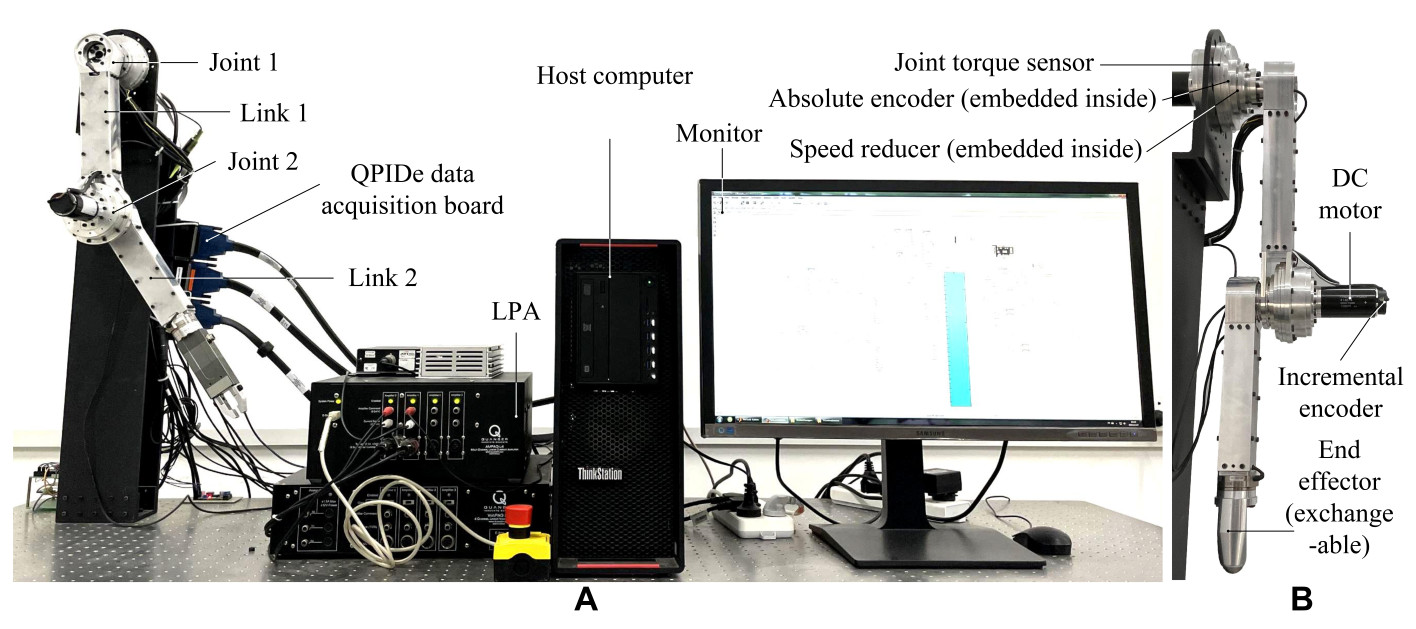
An experimental setup comprising a 2-degree-of-freedom modular robotic system is assembled to evaluate the performance of the proposed decentralized robust neural network controller, as illustrated in Figure 1. The actuation unit consists of a brushed DC motor (Maxon 218014) with a maximum rated torque of 190 mN·m and a torque constant of 0.321 N·m/A. Motor driving is accomplished via a linear power amplifier (LPA, Quanser Inc.), and experimental data acquisition is performed using a QPIDe data acquisition board from the same manufacturer. A harmonic drive with a transmission ratio of 101:1 couples the motor output to the joint mechanism. Motor-side position feedback is obtained from a 500-line incremental encoder supplied with the Maxon motor, while link-side torque measurements are acquired through torque estimation. In the experiment process, a torque sensor is not used. A torque sensor is supplied for verifying the correctness of the harmonic drive estimation. The QUARC software suite (Quanser Inc.) integrates natively with Simulink and communicates with the QPIDe board, thereby supporting both the logging of data from external instrumentation and its subsequent manipulation within the Simulink environment. The upper bounds of the module and controller parameters and uncertainty used in the experiment are given in Table 1.
Learning-based robust control of modular robot manipulators: an experimental investigation

Figure 1. Experimental setup (A) platform (B) moudle. LPA: Linear power amplifier.

The reference trajectory prescribed for joint 1 is given by

$$ \begin{equation} {{q}_{id}}\left( t \right)=\frac{20\pi }{180}\sin \left( \frac{\pi }{18}t \right) \end{equation} $$

The reference trajectory prescribed for joint 2 is given by

$$ \begin{equation} {{q}_{id}}\left( t \right)=\frac{20\pi }{180}\sin \left( \frac{\pi }{10}t \right) \end{equation} $$

RESULTS AND DISCUSSION

Trajectory tracking

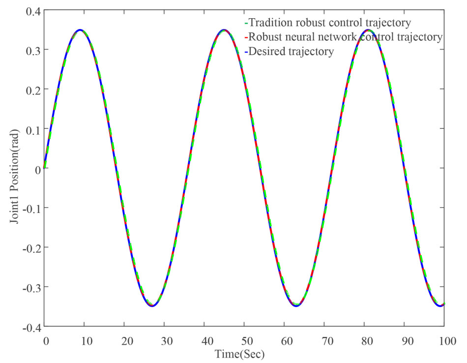
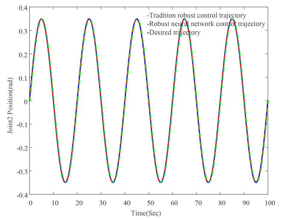
Figures 2 and 3 present the trajectory tracking curves of the modular robot. This part of the experiment compares the trajectory-tracking performance of the conventional robust control method [26-28] with that of the proposed robust neural network control method. The experimental curves indicate that, while both control methods are capable of tracking the desired trajectory reasonably well, the conventional robust control method still exhibits relatively large tracking errors at certain points along the trajectory. In contrast, the robust neural network-based control method achieves superior trajectory-tracking performance, owing to its ability to more accurately approximate the MRM model and compensate for model uncertainties.
Learning-based robust control of modular robot manipulators: an experimental investigation

Figure 2. Joint 1 trajectory tracking.
Learning-based robust control of modular robot manipulators: an experimental investigation

Figure 3. Joint 2 trajectory tracking.

Trajectory tracking error

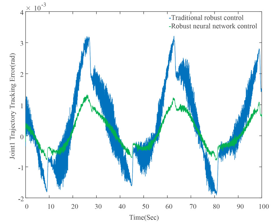
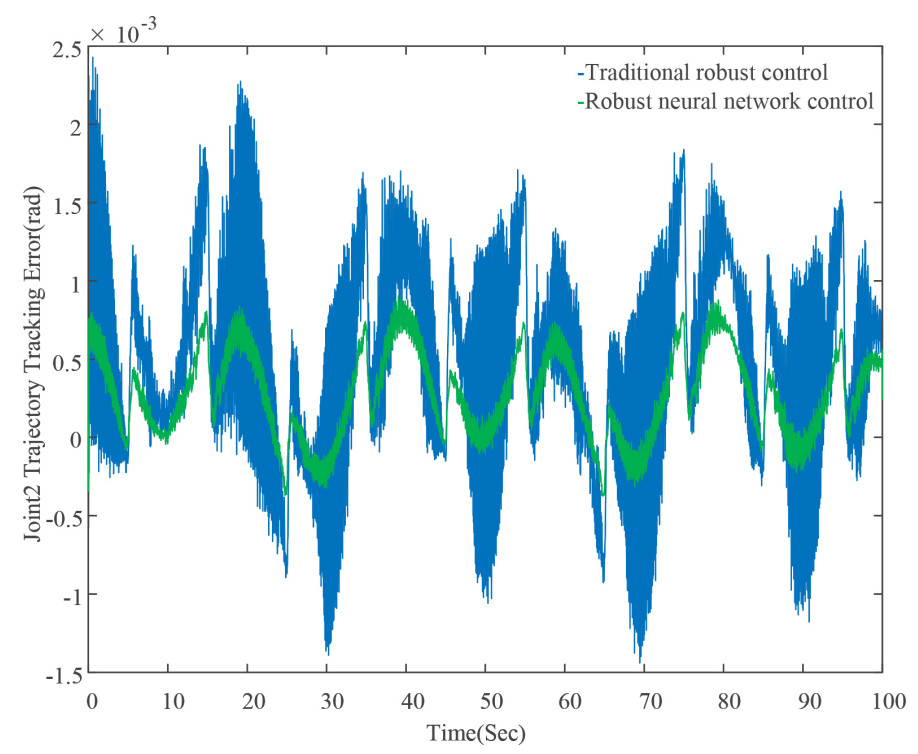
Figures 4 and 5 present the trajectory tracking error curves of the modular robot. This segment of the experiment compares the tracking errors obtained using the conventional robust control method with those achieved by the robust neural network control method proposed in this paper. The experimental curves clearly indicate that a pronounced chattering effect is evident in the error profile when the conventional robust control method is employed. By contrast, owing to the neural network's capacity to approximate and compensate for model uncertainties and coupling terms, the proposed robust neural network control method accomplishes accurate compensation of model uncertainties, thereby effectively suppressing joint chattering, reducing control error, and yielding superior control accuracy. As a result, the trajectory tracking performance of both joints is substantially enhanced.
Learning-based robust control of modular robot manipulators: an experimental investigation

Figure 4. Joint 1 trajectory tracking error.
Learning-based robust control of modular robot manipulators: an experimental investigation

Figure 5. Joint 2 trajectory tracking error.

Motor output torque

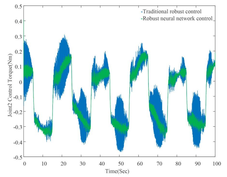
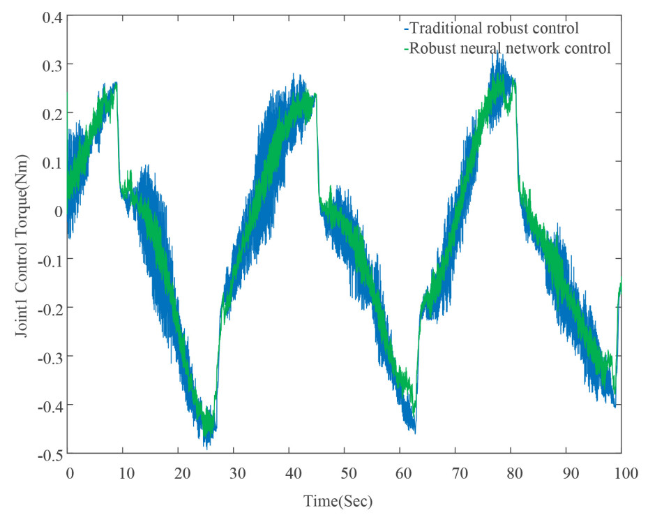
Figures 6 and 7 present the motor output torque curves of the modular robot. This part of the experiment compares the motor output torque obtained using the traditional robust control method with that obtained using the robust neural network control method proposed in this paper. It can be observed from the experimental curves that the motor output torque under the traditional robust control method exhibits a pronounced chattering effect, whereas the motor output torque under the proposed robust neural network control method is relatively smooth. The control torque root mean square of the joint 1’s existed method is 0.18, and the developed method is 0.12. The control torque root mean square of the joint 2’s existed method is 0.2, and the developed method is 0.12. The value of root mean square is suppressed by about 35%. The calculate method is as follows: $$ \left( 0.18-0.12 \right)/0.18\approx 33.3\%, \left( 0.2-0.12 \right)/0.2\approx 40\%. $$
Learning-based robust control of modular robot manipulators: an experimental investigation

Figure 6. Joint 1 control torque.

Learning-based robust control of modular robot manipulators: an experimental investigation

Figure 7. Joint 2 control torque.

NN weight

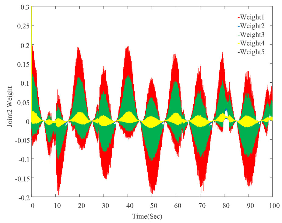
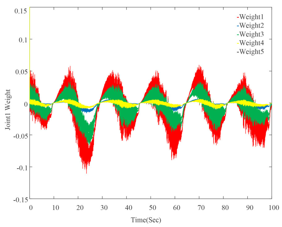
Figures 8 and 9 depict the weight variation curves of the neural network for joint 1 and joint 2 of the modular robot, respectively. In this experiment, five neural nodes were configured to approximate the model uncertainties of the robot. As can be observed from the experimental curves, the neural network weights oscillate in a regular manner within a bounded range.
Learning-based robust control of modular robot manipulators: an experimental investigation

Figure 8. Joint 1 Weight.

Learning-based robust control of modular robot manipulators: an experimental investigation

Figure 9. Joint 2 Weight.

CONCLUSIONS

This paper presents a robust neural network-based control method for modular robot manipulators. The controller compensates for friction modeling errors through robust control, while a neural network is employed to simultaneously approximate and compensate for the remaining model uncertainties - including the IDC term, the torque transmission deviation of the harmonic drive, and the measurement disturbance, and to mitigate controller chattering. The asymptotic stability of the resulting closed-loop system is rigorously established via Lyapunov analysis, and the efficacy of the proposed robotic control strategy is substantiated by experimental results.

The proposed control method is based on a time-triggered approach with a fixed cycle. Once the system reaches a stable state, the periodic triggering will waste communication resources. Therefore, an event-triggered control method that varies with time for sampling will be our future research direction.

DECLARATIONS

Authors' contributions

Made substantial contributions to conception and design of the study and performed data analysis and interpretation: Ji, Z.

Performed data acquisition, as well as provided administrative, technical, and material support: An, T.

Availability of data and materials

The data presented in this study are available on request from the corresponding author because the experimental data were generated by the experimental platform and cannot be used independently.

AI and AI-assisted tools statement

Not applicable.

Financial support and sponsorship

The work is supported by the Scientific Technological Development Plan Project in Jilin Province of China (20260602029RC).

Conflicts of interest

All authors declared that there are no conflicts of interest.

Ethical approval and consent to participate

Not applicable.

Consent for publication

Not applicable.

Copyright

The Author(s) 2026.

REFERENCES

1. Lei, Z.; Shi, J.; Luo, Z.; Cheng, M.; Wan, J. Intelligent manufacturing from the perspective of industry 5.0: application review and prospects. IEEE. Access. 2024, 12, 167436-51.

2. Xiang, W.; Yu, K.; Han, F.; Fang, L.; He, D.; Han, Q. L. Advanced manufacturing in industry 5.0: a survey of key eenabling technologies and future trends. IEEE. Trans. Ind. Inf. 2024, 20, 1055-68.

3. Lou, S.; Hu, Z.; Zhang, Y.; Feng, Y.; Zhou, M.; Lv, C. Human-cyber-physical system for industry 5.0: a review from a human-centric perspective. IEEE. Trans. Automat. Sci. Eng. 2025, 22, 494-511.

4. Uno, K.; Neppel, E.; Diaz, G. H.; et al. MoonBot: modular and on-demand reconfigurable robot toward moon base construction. IEEE. Trans. Field. Robot. 2025, 2, 847-74.

5. Ji, Z.; Ma, B.; Jiang, H.; Liang, J.; Dong, B.; An, T. Event-triggered-based optimal control for reconfigurable robot via mixed nonzero-sum game. IFAC-PapersOnLine 2025, 59, 332-7.

6. Iqbal, J.; Ahmad, O.; Malik, A. HEXOSYS Ⅱ - towards realization of light mass robotics for the hand. In: 2011 IEEE 14th International Multitopic Conference (INMIC), Karachi, Pakistan, November 22-24, 2011. IEEE; 2011, 115-119. DOI: 10.1109/INMIC.2011.6151454.

7. An, T.; Wang, Y.; Liu, G.; Li, Y.; Dong, B. Cooperative game-based approximate optimal control of modular robot manipulators for human–robot collaboration. IEEE. Trans. Cybern. 2023, 53, 4691-703.

8. Taghirad, H.; Belanger, P. Intelligent built-in torque sensor for harmonic drive systems. IEEE. Trans. Instrum. Meas. 1999, 48, 1201-7.

9. Zhang, H.; Ahmad, S.; Liu, G. Modeling of torsional compliance and hysteresis behaviors in harmonic drives. IEEE/ASME. Trans. Mechatron. 2015, 20, 178-85.

10. Zhang, H.; Ahmad, S.; Liu, G. Torque estimation for robotic joint with harmonic drive transmission based on position measurements. IEEE. Trans. Robot. 2015, 31, 322-30.

11. Jung, B. j.; Kim, B.; Koo, J. C.; Choi, H. R.; Moon, H. Joint torque sensor embedded in harmonic drive using order tracking method for robotic application. IEEE/ASME. Trans. Mechatron. 2017, 22, 1594-9.

12. Berghuis, H.; Nijmeijer, H. Robust control of robots via linear estimated state feedback. IEEE. Trans. Automat. Contr. 1994, 39, 2159-62.

13. Dong, B.; An, T.; Zhou, F.; Liu, K.; Yu, W.; Li, Y. Actor-critic-identifier structure-based decentralized neuro-optimal control of modular robot manipulators with environmental collisions. IEEE. Access. 2019, 7, 96148-65.

14. Li, X.; Song, C.; Yang, Y.; Zhu, C.; Liao, D. Optimal design of wave generator profile for harmonic gear drive using support function. Mech. Mach. Theory. 2020, 152, 103941.

15. Megalingam, R. K.; Vadivel, S. R. R.; Manoharan, S. K.; Pula, B. T.; Sathi, S. R.; Gupta, U. S. C. Reduced kinematic error for position accuracy in a high-torque, lightweight actuator. Actuators. 2024, 13, 218.

16. Liu, G.; Abdul, S.; Goldenberg, A. A. Distributed control of modular and reconfigurable robot with torque sensing. Robotica 2008, 26, 75-84.

17. Iqbal, U.; Samad, A. N. A.; Nlssa, Z.; Iqbal, J. Embedded control system for AUTAREP - a novel AUTonomous articulated robotic educational platform. Teh. Vjesn. 2014, 21, 1255-61. https://www.researchgate.net/publication/280641667_Embedded_control_system_for_AUTAREP_-_A_novel_AUTonomous_Articulated_Robotic_Educational_Platform [Last accessed on 15 July 2026].

18. Shen, M.; Wang, Z.; Zhu, S.; Zhao, X.; Zong, G.; Wang, Q. G. Neural network adaptive iterative learning control for strict-feedback unknown delay systems against input saturation. IEEE. Trans. Neural. Netw. Learning. Syst. 2025, 36, 13460-9.

19. Wang, C.; Zhang, H.; Wen, D.; Shen, M.; Li, L.; Zhang, Z. Novel passivity and dissipativity criteria for discrete-time fractional generalized delayed Cohen-Grossberg neural networks. Commun. Nonlinear. Sci. 2024, 133, 107960.

20. Shen, M.; Wu, X.; Park, J. H.; Yi, Y.; Sun, Y. Iterative learning control of constrained systems with varying trial lengths under alignment condition. IEEE. Trans. Neural. Netw. Learning. Syst. 2023, 34, 6670-6.

21. Dong, B.; An, T.; Zhou, F.; Liu, K.; Li, Y. Decentralized robust zero-sum neuro-optimal control for modular robot manipulators in contact with uncertain environments: theory and experimental verification. Nonlinear. Dyn. 2019, 97, 503-24.

22. Dong, B.; Liu, K.; Li, Y. Decentralized control of harmonic drive based modular robot manipulator using only position measurements: theory and experimental verification. J. Intell. Robot. Syst. 2017, 88, 3-18.

23. Wang, Y.; An, T.; Cui, Y.; Li, Y.; Dong, B. Decentralized position/torque control of modular robot manipulators via interaction torque estimation-based human motion intention identification. Int. J. Control. Autom. Syst. 2024, 22, 1585-600.

24. Dong, B.; Wang, Y.; An, T.; Cui, Y.; Zhu, X. Adaptive torque estimation-based nonlinear H $$\infty$$ control of modular robot manipulators with uncertain environments. Neural. Comput. &. Applic. 2024, 37, 1617-31.

25. Ma, B.; Dong, B.; Zhou, F.; Li, Y. Adaptive dynamic programming-based fault-tolerant position-force control of constrained reconfigurable manipulators. IEEE. Access. 2020, 8, 183286-99.

26. Daş, E.; Burdick, J. W. Robust control barrier functions using uncertainty estimation with application to mobile robots. IEEE. Trans. Automat. Contr. 2025, 70, 4766-73.

27. Zeng, D.; Jiang, Y.; Wang, Y.; Zhang, H.; Feng, Y. Robust adaptive control barrier functions for input-affine systems: application to uncertain manipulator safety constraints. IEEE. Control. Syst. Lett. 2024, 8, 279-84.

28. Li, X.; Kui, Q.; Yao, W.; Wu, L. Robust parallel cooperative control of cable-driven robot system via adaptive integral sliding mode. IEEE. Robot. Autom. Lett. 2025, 10, 5433-40.

Cite This Article

Research Article
Open Access
Learning-based robust control of modular robot manipulators: an experimental investigation

How to Cite

Download Citation

If you have the appropriate software installed, you can download article citation data to the citation manager of your choice. Simply select your manager software from the list below and click on download.

Export Citation File:

Type of Import

Tips on Downloading Citation

This feature enables you to download the bibliographic information (also called citation data, header data, or metadata) for the articles on our site.

Citation Manager File Format

Use the radio buttons to choose how to format the bibliographic data you're harvesting. Several citation manager formats are available, including EndNote and BibTex.

Type of Import

If you have citation management software installed on your computer your Web browser should be able to import metadata directly into your reference database.

Direct Import: When the Direct Import option is selected (the default state), a dialogue box will give you the option to Save or Open the downloaded citation data. Choosing Open will either launch your citation manager or give you a choice of applications with which to use the metadata. The Save option saves the file locally for later use.

Indirect Import: When the Indirect Import option is selected, the metadata is displayed and may be copied and pasted as needed.

About This Article

Special Topic

Disclaimer/Publisher’s Note: All statements, opinions, and data contained in this publication are solely those of the individual author(s) and contributor(s) and do not necessarily reflect those of OAE and/or the editor(s). OAE and/or the editor(s) disclaim any responsibility for harm to persons or property resulting from the use of any ideas, methods, instructions, or products mentioned in the content.
© The Author(s) 2026. Open Access This article is licensed under a Creative Commons Attribution 4.0 International License (https://creativecommons.org/licenses/by/4.0/), which permits unrestricted use, sharing, adaptation, distribution and reproduction in any medium or format, for any purpose, even commercially, as long as you give appropriate credit to the original author(s) and the source, provide a link to the Creative Commons license, and indicate if changes were made.

Data & Comments

Data

Views
15
Downloads
4
Citations
0
Comments
0
0

Comments

Comments must be written in English. Spam, offensive content, impersonation, and private information will not be permitted. If any comment is reported and identified as inappropriate content by OAE staff, the comment will be removed without notice. If you have any queries or need any help, please contact us at [email protected].

0
Download PDF
Share This Article
Scan the QR code for reading!
See Updates
Contents
Figures
Related
Intelligent Control Systems
ISSN : XXXX-XXXX (Coming soon)
Navigation
Navigation