Download PDF
Research Article  |  Open Access  |  14 Jul 2026

Projective synchronization analysis of multiple-time-scale competitive neural networks in quaternion field

Views: 21 |  Downloads: 5 |  Cited:  0
Intell. Control Syst. 2026, 1, 2.
10.20517/ics.2026.03 |  © The Author(s) 2026.
Author Information
Article Notes
Cite This Article

Abstract

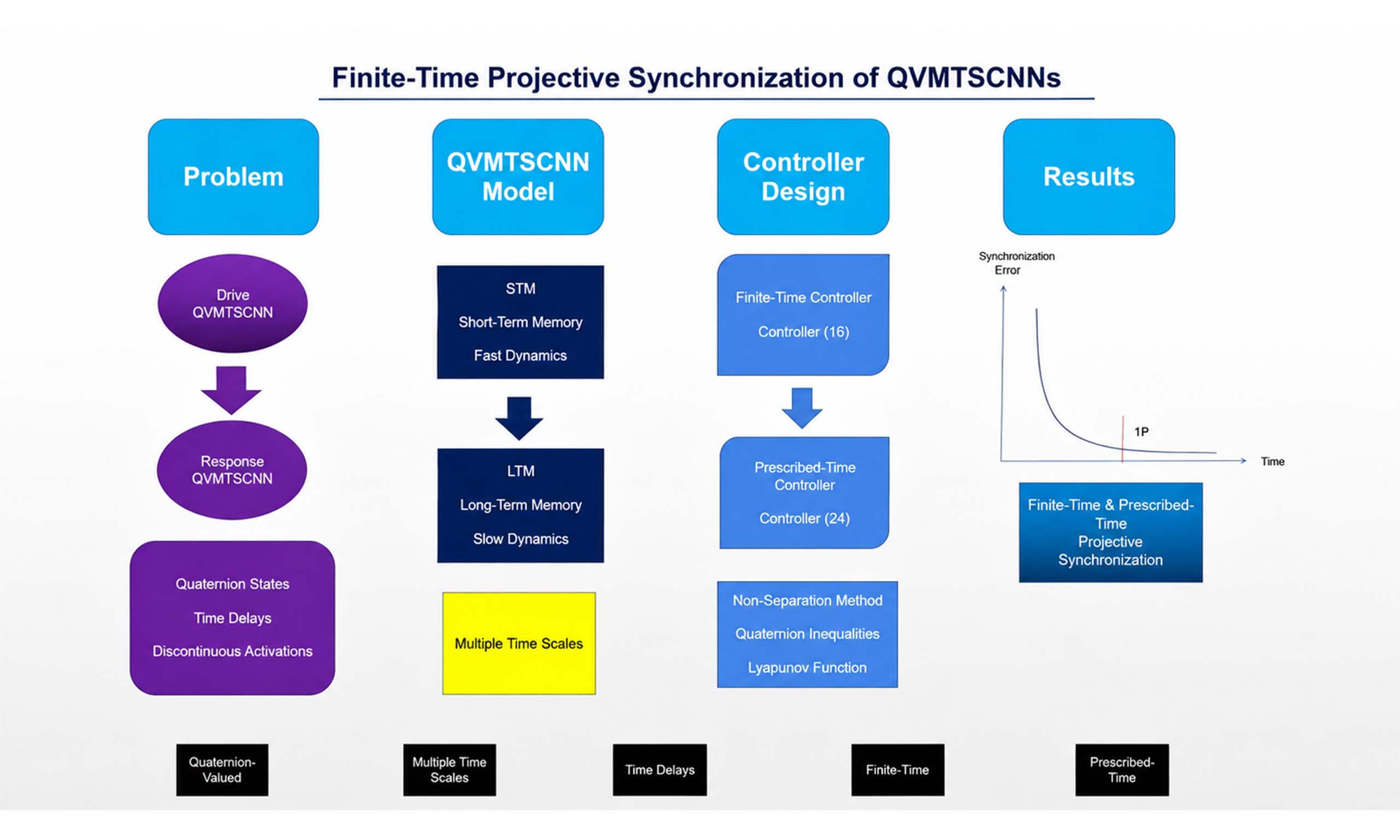
This work proposes the model of quaternion-valued multiple-time-scale competitive neural networks (QVMTSCNNs) for the first time and explores the projective synchronization problem of it. Due to the existence of multiple time scale and quaternion, the previous control method cannot be directly used. Thus, two novel control strategies are designed to investigate the finite-time/prescribed-time projective synchronization issue. Using non-separation method, novel criteria for finite-time/prescribed-time projective synchronization of QVMTSCNNs are derived by using the nonsmooth theory and quaternion inequality skills. Lastly, simulations are given to verify our results.

Keywords

Multiple time scales, quaternion, competitive neural networks, finite-time synchronization, prescribed-time synchronization

INTRODUCTION

Recently, the dynamics of competitive neural networks (CNNs) have received significant attention for their broad application. Later, the model of CNNs on multiple time scales (MTSCNNs) was proposed in[1]. There are two kinds of memories in MTSCNNs: the long-term memory (LTM), which describes slow synaptic modifications, and the short-term memory (STM), which describes the rapid dynamics of the neuron activity. The MTSCNNs model shows promising prospects in pattern recognition, neural computing, and visual processing[2]. Particularly, MTSCNNs can be described as a singularly perturbed system on multiple time scales[3,4,5,6,7].

Quaternions were first proposed by Hamilton in 1843[8]. Later, quaternions have shown broad application in fields such as aerospace technology, pattern recognition, and digital processing[9,10]. Recently, to improve color image processing, quaternion-valued neural networks (QVNNs) were created[11], where the neuron state is denoted by a quaternion. Compared with real-valued neural networks, QVNNs can process four-dimensional information in an integrated manner and preserve the intrinsic coupling relationships among different components. Therefore, they have demonstrated significant advantages in color image processing, attitude representation, signal processing and multidimensional data fusion. Lately, the dynamical analysis of QVNNs has received considerable attention[12,13,14]. However, most of these papers considered the dynamical systems evolving on one time scale; the multiple time scales have not been considered yet.

In the past, investigations of the dynamics of CNNs mainly focused on the case of one time scale. However, multiple time scales are more common in the signal communication between the neuron nodes, causing dynamics to be complex[15,16]. Research on networks across multiple time scales can extend many existing works, which is a challenging direction. Moreover, different from the traditional issue of complete synchronization, projective synchronization gives better performance in fast transmission because of the proportional and adjustable relation between drive-response networks[17,18,19]. Furthermore, most previous results considered the projective coefficient as real-valued. Compared with a real projective coefficient, the quaternion-valued projective parameter can improve the complexity and diversity of synchronization.

Synchronization theory serves as a core component in analyzing the stability and robustness of nonlinear systems[20]. Recently, the finite-time synchronization (FTS) has been proposed, and it can guarantee system performance within an initial-state-dependent finite time interval. However, due to its dependence on initial conditions, the FTS may be insufficient when the initial conditions are unknown or very large[21,22,23]. To overcome this limitation, the fixed-time synchronization (FXTS) was proposed[24], which ensures that the convergence time can be estimated by a fixed number independent of initial conditions. However, there is a limitation of the FXTS method: its settling time is dependent on the system parameters[25,26,27,28,29,30,31], which remains a huge restriction for real applications. To overcome this shortage, the PTS control is put forward[32,33,34], where the convergence time can be preassigned only by humans, which is quite flexible and applicable in engineering. Due to the complexity of the network model, the FXTS and PTS problem of QVNNs on multiple time scales has not been considered yet, which remains a challenging direction.

Furthermore, in most existing papers, the activation function of neurons is usually assumed as continuous[21,22,23,24,25,26,27,28,29,30,31]. But in practice, discontinuous activation functions are more applicable because of the system oscillating and dry friction[26,31]. In fact, discontinuous neural systems can be applied to fields of optimization, power circuits, control problems, and so forth. Thus, it is practical to consider the discontinuous functions in our research.

As we know, the issue of projective synchronization for QVNNs with multiple time scales has not yet been addressed. This work aims to explore the projective FTS and PTS problem of this network. The main points are listed as follows.

(1) In this work, the QVMTSCNNs model is proposed for the first time, which extends the dynamics of traditional MTSCNNs to the quaternion field. The previous results in[17,18,19] can be seen as a particular case of this work.

(2) Two novel synchronizing controllers are proposed to cope with the difficulty caused by multiple time scales; the problem of projective FTS and PTS for QVMTSCNNs is solved for the first time.

(3) The effects of discontinuous activations and transmission delays are simultaneously considered, the proposed model is more realistic and broadens the applicability of the obtained synchronization criteria.

Notations. $$ \mathbb{R} $$ and $$ \mathbb{Q} $$ denote the real and quaternion numbers. For $$ \kappa=\kappa^{R}+j\kappa^{J}+i\kappa^{I}+k\kappa^{K}\in\mathbb{Q} $$, the conjugate of $$ \kappa $$ is $$ \kappa^{*}=\kappa^{R}-i\kappa^{I}-j\kappa^{J}-k\kappa^{K} $$, the 1-norm of $$ \kappa\in\mathbb{Q} $$ is defined as $$ \|\kappa\|_{1}=|\kappa^{R}|+|\kappa^{I}|+|\kappa^{J}|+|\kappa^{K}| $$, the 2-norm of $$ \kappa\in\mathbb{Q} $$ is $$ \|\kappa\|_{2}=\sqrt{\kappa^{*}\kappa} $$. For $$ w\in\mathbb{Q} $$, define the quaternion sign function as $$ [w]=sgn(w^{R})+isgn(w^{I})+jsgn(w^{J})+ksgn(w^{K}) $$. For $$ \eta=(\eta_{1}, \cdots, \eta_{M})^{T}\in\mathbb{Q}^{M} $$ and $$ q > 0 $$, make the following definition: $$ sgn(\eta)=(sgn(\eta_{1}), \cdots, sgn(\eta_{M}))^{T} $$, $$ [\eta]^{q}=([\eta_{1}]^{q}, \cdots, [\eta_{M}]^{q})^{T}\in\mathbb{Q}^{M} $$, where $$ [\eta_{i}]^{q}=sgn(\eta_{i})\|\eta_{i}\|^{q}_{1} $$.

PRELIMINARIES

For $$ \chi\in \mathbb{Q} $$, it has

$$ \chi=\chi^{R}+\chi^{I}i+\chi^{J}j+\chi^{K}k, $$

where $$ \chi^{R}, \chi^{J}, \chi^{I}, \chi^{K}\in \mathbb{R} $$. Furthermore, the Hamilton rule holds:

$$ \begin{align} &k=-ji=ij, i=-kj=jk, \\ &j=-ik=ki, i^{2}=j^{2}=k^{2}=-1.\end{align} $$

Consider the model of QVMTSCNNs:

$$ \begin{align} STM: \epsilon \dot{x}_{m}(t)=&-c_{m}x_{m}(t)+\sum\limits_{k=1}^{N}a_{mk}f_{k}(x_{k}(t))+\sum\limits_{k=1}^{N}b_{mk}f_{k}(x_{k}(t-\tau_{k}))\\ &+d_{m}S_{m}(t)\\ LTM: \dot{S}_{m}(t)=&-\alpha_{m}S_{m}(t)+\beta_{m}f_{m}(x_{m}(t))\end{align} $$

where $$ m=1, \cdots, N $$; $$ x_{m}(t) $$, $$ S_{m}(t)\in\mathbb{Q} $$ denote the activity level and external stimulus. $$ \tau_{k}\leq\tau $$ denotes time delay. $$ c_{m} > 0 $$; $$ \alpha_{m}, \beta_{m}\in\mathbb{R} $$ are constants. $$ f_{k}(\cdot) \in \mathbb{Q} $$ represents the activation function. $$ d_{m}\in\mathbb{R} $$ denotes the external stimulus. $$ \epsilon $$ is the time scale coefficient of the STM state. $$ a_{mk}, b_{mk}\in \mathbb{Q} $$ denote the connection weights strength between the $$ m $$th node and the $$ k $$th node. The initial value of (1) is $$ x_{m}(s)=\phi_{m}(s), S_{m}(s)=\Psi_{m}(s), -\tau\leq s\leq0 $$.

Considering the drive-response synchronization, take (1) as drive system, choose the controlled response system

$$ \begin{align} STM: \epsilon \dot{y}_{m}(t)=&-c_{m}y_{m}(t)+\sum\limits_{k=1}^{N}a_{mk}f_{k}(y_{k}(t))+\sum\limits_{k=1}^{N}b_{mk}f_{k}(y_{k}(t-\tau_{k}))\\ &+d_{m}R_{m}(t)+u_{m}(t)\\ LTM: \dot{R}_{m}(t)=&-\alpha_{m}R_{m}(t)+\beta_{m}f_{m}(y_{m}(t))+v_{m}(t) \end{align} $$

where $$ y_{m}(t), R_{m}(t)\in\mathbb{Q} $$ denote the states of slave system (2), $$ u_{m}(t), v_{m}(t)\in \mathbb{Q} $$ are the control inputs. The initial condition of (2) is $$ y_{m}(s)=\tilde{\phi}_{m}(s), R_{m}(s)=\tilde{\Psi}_{m}(s), -\tau\leq s\leq0 $$.

Remark 1 Note that, extending MTSCNNs from the real domain to the quaternion domain is nontrivial. Due to the noncommutativity of quaternion multiplication and the coupling among quaternion components, many existing analysis techniques for real-valued MTSCNNs cannot be directly applied[2,3,4]. Consequently, the stability analysis and controller design become much more challenging. Therefore, studying the dynamics of QVMTSCNNs is both theoretically meaningful and practically important.

Our aim is to realize the projective synchronization of above systems. Using differential inclusion theory, we set the assumptions for activation function.

Assumption 2.1. $$ f_{m}(x_{m})=f^{R}_{m}(x_{m})+if^{I}_{m}(x_{m})+jf^{J}_{m}(x_{m})+kf^{K}_{m}(x_{m}) $$ is continuous except for a countable number of points $$ \delta^{\iota}_{m} $$, the left and right limits $$ f^{S-}_{m}(\delta^{\iota}_{m}) $$ and $$ f^{S+}_{m}(\delta^{\iota}_{m}) $$ exist.

Assumption 2.2. For any $$ x_{k}, y_{k}\in\mathbb{Q} $$, there exist positive constants $$ l_{kl}, H_{kl}, M_{kl} $$ satisfying

$$ \|\gamma_{k}-\zeta_{k}\|_{l}\leq l_{kl}\|y_{k}-x_{k}\|_{l}+H_{kl}, \|f_{k}(y_{k})\|_{l}\leq M_{kl}, \; l=1, 2 $$

where $$ \gamma_{k}\in\overline{co}[f_{k}(y_{k})] $$, $$ \zeta_{k}\in\overline{co}[f_{k}(x_{k})] $$, $$ \overline{co}[f_{k}(\cdot)]=\overline{co}[f^{R}_{k}(\cdot)]+\overline{co}[f^{I}_{k}(\cdot)]i+\overline{co}[f^{J}_{k}(\cdot)]j+\overline{co}[f^{K}_{k}(\cdot)]k $$, $$ \overline{co}[f^{S}_{k}(\cdot)]=[\min\{f^{S-}_{k}(\cdot), f^{S+}_{k}(\cdot)\}, \max\{f^{S-}_{k}(\cdot), f^{S+}_{k}(\cdot)\}] $$, $$ S=R, I, J, K $$.

Due to the discontinuous functions in system (1), the traditional solution does not exist. We give the following definition.

Definition 1 $$ x(t)\in\mathbb{Q}^{n} $$ is named a Filippov solution of the network (1) on $$ [-\tau, T_{0}) $$, if

(1) $$ x(t) $$ is absolutely continuous on $$ [0, T_{0}) $$.

(2) There exist measurable functions $$ \zeta_{k}(t)\in\overline{co}[f_{k}(x_{k}(t))] $$ such that

$$ \begin{align} STM: \epsilon \dot{x}_{m}(t)=&-c_{m}x_{m}(t)+\sum\limits_{k=1}^{n}a_{mk}\zeta_{k}(t)+\sum\limits_{k=1}^{n}b_{mk}\zeta_{k}(t-\tau_{k})+d_{m}S_{m}(t)\\ LTM: \dot{S}_{m}(t)=&-\alpha_{m}S_{m}(t)+\beta_{m}\zeta_{m}(t) \end{align} $$

For slave system (2), there exist measurable functions $$ \varpi_{k}(t)\in\overline{co}[f_{k}(y_{k}(t))] $$ such that

$$ \begin{align} STM: \epsilon \dot{y}_{m}(t)=&-c_{m}y_{m}(t)+\sum\limits_{k=1}^{N}a_{mk}\varpi_{k}(t)+\sum\limits_{k=1}^{N}b_{mk}\varpi_{k}(t-\tau_{k}))\\ &+d_{m}R_{m}(t)+u_{m}(t)\\ LTM: \dot{R}_{m}(t)=&-\alpha_{m}R_{m}(t)+\beta_{m}\gamma_{m}(t)+v_{m}(t)\end{align} $$

Next, we consider the projective synchronization of above systems. Let $$ \lambda_{m}\in\mathbb{Q} $$ be a projective coefficient. Define

$$ z_{m}(t)=y_{m}(t)-\lambda_{m}x_{m}(t), \varepsilon_{m}(t)=R_{m}(t)-\lambda_{m}S_{m}(t) $$

as the projective synchronization error. Then we obtain the error dynamics:

$$ \begin{align} \epsilon \dot{z}_{m}(t)=&-c_{m}z_{m}(t)+\sum\limits_{k=1}^{N}a_{mk}(\varpi_{k}(t)-\delta_{k}(t))+\sum\limits_{k=1}^{N}a_{mk}(\delta_{k}(t)-\lambda_{m}\zeta_{k}(t))\\ &+\sum\limits_{k=1}^{N}b_{mk}(\varpi_{k}(t-\tau_{k})-\delta_{k}(t-\tau_{k}))+\sum\limits_{k=1}^{N}b_{mk}(\delta_{k}(t-\tau_{k})-\lambda_{m}\zeta_{k}(t-\tau_{k}))\\ &+d_{m}\varepsilon_{m}(t)+u_{m}(t)\\ \dot{\varepsilon}_{m}(t)=&-\alpha_{m}\varepsilon_{m}(t)+\beta_{m}(\gamma_{m}(t)-\lambda_{m}\zeta_{m}(t))+v_{m}(t) \end{align} $$

where $$ \varpi_{k}(t)\in\overline{co}[f_{k}(y_{k}(t))], \delta_{k}(t)\in\overline{co}[f_{k}(\lambda_{m}x_{k}(t))], \zeta_{k}(t)\in\overline{co}[f_{k}(x_{k}(t))] $$.

Lemma 1 [31] For $$ \kappa, \omega\in\mathbb{Q}^{n} $$, we have

$$ \begin{align} &(1)\; \kappa^{*}[\kappa]+[\kappa]^{*}\kappa=2\|\kappa\|_{1}\\ &(2)\; \|\kappa^{*}\omega\|_{1}\leq\|\kappa\|_{1}\|\omega\|_{1}, \; \|\kappa^{*}\omega\|_{2}\leq\|\kappa\|_{2}\|\omega\|_{2}\\ &(3)\; \frac{1}{2}(\kappa^{*}\omega+\omega^{*}\kappa)=(\kappa^{*}\omega)^{R}\leq\|\kappa\|_{2}\|\omega\|_{2}\\ &(4)\; D^{+}\big([\kappa(t)]^{*}\kappa(t)+\kappa(t)^{*}[\kappa(t)]\big)\\ &=[\kappa(t)]^{*}\dot{\kappa}(t)+\dot{\kappa}(t)^{*}[\kappa(t)], \|\kappa(t)\|_{1}\neq0 \end{align} $$

where $$ [\kappa] $$ denotes the sign function of $$ \kappa $$.

Definition 2 Given $$ \epsilon > 0 $$, system (1) and (2) are said to reach projective FTS, if there exists $$ T_{0}(\epsilon) > 0 $$, such that

$$ \begin{align} &\lim\limits_{s\rightarrow T_{0}(\epsilon)}\|z_{m}(s)\|_{l}=\lim\limits_{s\rightarrow T_{0}(\epsilon)}\|\varepsilon_{m}(s)\|_{l}=0, \; m=1, \cdots, N\\ &\|z_{m}(s)\|_{l}=\|\varepsilon_{m}(s)\|_{l}=0, \; \forall s\in[T_{0}(\epsilon), +\infty).\end{align} $$

where $$ l=1, 2 $$, $$ T_{0}(\epsilon) $$ is related to initial system condition. Moreover, (1) and (2) are said to reach projective FXTS, if $$ T_{0}(\epsilon) < T_{\max}(\epsilon) $$, where $$ T_{\max}(\epsilon) $$ is independent on initial system condition, but may be related with the coefficients in system and controller.

Definition 3 The systems (1) and (2) are said to reach projective PTS, if there exists $$ T_{p} > 0 $$, such that

$$ \begin{align} &\lim\limits_{s\rightarrow T_{p}}\|z_{m}(s)\|_{l}=\lim\limits_{s\rightarrow T_{p}}\|\varepsilon_{m}(s)\|_{l}=0, \; m=1, \cdots, N\\ &\|z_{m}(s)\|_{l}=\|\varepsilon_{m}(s)\|_{l}=0, \; \forall s\in[T_{p}, +\infty). \end{align} $$

where $$ l=1, 2 $$, $$ T_{p} $$ is independent on both initial values and system coefficients.

Lemma 2 [31]

Assume $$ V(s): \mathbb{R}^{n}\rightarrow \mathbb{R}^{+} $$ is continuous, if there are constants $$ q_{1} > 0 $$, $$ 0\leq\alpha < 1 $$ satisfy

$$ \dot{V}(s)\leq-q_{1}V^{\alpha}(s)\; , \; s\geq0 $$

Then,

$$ V^{1-\alpha}(s)\leq V^{1-\alpha}(0)-q_{1}(1-\alpha)s\; , \; 0\leq s\leq T $$

and $$ V(s)\equiv0 $$ for $$ s\geq T $$, and

$$ T\leq\frac{V^{1-\alpha}(0)}{q_{1}(1-\alpha)} $$

Lemma 3 [31]

Assume $$ V(s): \mathbb{Q}^{n}\rightarrow \mathbb{R}^{+} $$ is continuous, if

$$ \dot{V}(s)\leq -\mu-\kappa V^{r}(s)\; , \; s\in[t_{0}, +\infty) $$

where $$ \mu, \kappa, r\geq0 $$, then we can derive

(1) If $$ r=0 $$, then $$ V(s)\equiv0 $$ when $$ s\geq T_{1} $$, where

$$ T_{1}\leq \hat{T}_{1}=\frac{V(0)}{\mu+\kappa} $$

(2) If $$ 0 < r < 1 $$, $$ V(s)\equiv0 $$ when $$ s\geq T_{2} $$, where

$$ T_{2}\leq \hat{T}_{2}=\frac{1}{1-r}\Big(\frac{\mu^{1-r}}{\kappa}\Big)^{\frac{1}{r}}\Big(\Big(\Big(\frac{\kappa}{\mu}\Big)^{\frac{1}{r}}V(0)+1\Big)^{1-r}-1\Big) $$

(3) If $$ r=1 $$, then $$ V(s)\equiv0 $$ for $$ s\geq T_{3} $$, where

$$ T_{3}\leq \hat{T}_{3}=\frac{1}{\kappa}\ln\frac{\mu+\kappa V(0)}{\mu} $$

(4) If $$ r > 1 $$, then $$ V(s)\equiv0 $$ for $$ s\geq T_{4} $$, where

$$ T_{4}\leq \hat{T}_{4}=\frac{1}{\mu}\Big(\frac{\mu}{\kappa}\Big)^{\frac{1}{r}}\Big(1+\frac{1}{1-r}\Big) $$

Lemma 4 [18] Consider a continuous function $$ V(e(s)) $$: $$ \mathbb{Q}^{n}\rightarrow \{0\}\cup\mathbb{R}^{+} $$, if

(1) $$ e(s)=0 \Leftrightarrow V(e(s))=0 $$.

(2) The following condition holds for any solution $$ e(s)\in\mathbb{Q}^{n} $$ of network (6)

$$ \dot{V}(e(s))\leq-bV(e(s))-\hat{k}\varphi(s)V(e(s)), \; for\; s\geq t_{0} $$

Then the origin of (6) can be stable within a predefined time $$ T_{p} $$. Herein, $$ \hat{k} > 0, T_{p} > 0 $$ and $$ b < \frac{\hat{p}\hat{k}}{T_{p}} $$. Meanwhile, $$ \eta(s) $$ and $$ \varphi(s) $$ are given as:

$$ \begin{aligned} \varphi(s)=&\left\{\begin{array}{c} \frac{\dot{\eta}(s)}{\eta(s)}, \; s\in[t_{0}, t_{0}+T_{p}), \\ \; \; \; \; \frac{\hat{p}}{T_{p}}, \; s\in[t_{0}+T_{p}, +\infty), \end{array}\right. \end{aligned} $$

$$ \eta(s)=\frac{(T_{p})^{\hat{p}}}{(t_{0}+T_{p}-s)^{\hat{p}}}, \; s\in[t_{0}, t_{0}+T_{p}) $$

Lemma 5 For $$ z_{1}, \cdots, z_{\epsilon}\geq0, 0 < p < 1, q > 1 $$, it has

$$ \sum\limits_{\sigma=1}^{\epsilon}z^{p}_{\sigma}\geq(\sum\limits_{\sigma=1}^{\epsilon}z_{\sigma})^{p}, \sum\limits_{\sigma=1}^{\epsilon}z^{q}_{\sigma}\geq \epsilon^{1-q}(\sum\limits_{\sigma=1}^{\epsilon}z_{\sigma})^{q}. $$

RESULTS AND DISCUSSION

Now, we design the criteria for projective synchronization of QVMTSCNNs (1) and (2). Provide the control scheme:

$$ \begin{align} u_{m}(t)=&-k_{m}z_{m}(t)-\rho[z_{m}(t)]\|z_{m}(t)\|^{\delta}_{1}-[z_{m}(t)]\Big(\vartheta_{m}+\sum\limits_{k=1}^{N}\xi_{mk}\|z_{k}(t-\tau_{k})\|_{1}\Big)\\ v_{m}(t)=&-\eta_{m}\varepsilon_{m}(t)-\rho[\varepsilon_{m}(t)]\|\varepsilon_{m}(t)\|^{\delta}_{1} \end{align} $$

where $$ k_{m}, \eta_{m}, \vartheta_{m}, \xi_{mk}, \rho $$ are positive constants and $$ \delta\geq0 $$, $$ [z_{m}(t)], [\varepsilon_{m}(t)] $$ are sign functions of $$ z_{m}(t) $$ and $$ \varepsilon_{m}(t) $$.

Denote

$$ \begin{align} W=\min\limits_{m=1, \cdots, N}\Big\{&\vartheta_{m}-\sum\limits_{k=1}^{N}\Big((\|a_{mk}\|_{1}+\|b_{mk}\|_{1})(1+\|\lambda_{m}\|_{1})M_{k1}+\|a_{mk}\|_{1}H_{k1}\Big)\\ &-|\beta_{m}|H_{m1}-|\beta_{m}|(1+\|\lambda_{m}\|_{1})M_{m1}\Big\} \end{align} $$

Then, the theorem for quaternion projective synchronization of QVMTSCNNs is derived.

Theorem 1 With Assumption 2.1 and 2.2 and controller (16), for a given $$ \epsilon > 0 $$, if

$$ \begin{align} k_{m}\geq&-c_{m}+|\beta_{m}|l_{m1}+\sum\limits_{k=1}^{N}\|a_{km}\|_{1}l_{m1}, \; \eta_{m}\geq |d_{m}|-\alpha_{m}, \; \xi_{mk}\geq\|b_{mk}\|_{1}l_{k1}, \\ \vartheta_{m}\geq&\sum\limits_{k=1}^{N}\Big((\|a_{mk}\|_{1}+\|b_{mk}\|_{1})(1+\|\lambda_{m}\|_{1})M_{k1}+\|a_{mk}\|_{1}H_{k1}\Big)+|\beta_{m}|H_{m1}\\ &+|\beta_{m}|(1+\|\lambda_{m}\|_{1})M_{m1} \end{align} $$

the following results for quaternion projective synchronization can be obtained.

(1) For $$ W=0 $$, $$ 0 < \delta < 1 $$, the projective FTS of networks (1) and (2) can be achieved in $$ T_{1}(\epsilon) $$ estimated as

$$ T_{1}(\epsilon)\leq \hat{T}_{1}(\epsilon)=\frac{(1+\epsilon^{\delta})(\epsilon\|z_{0}\|_{1}+\|\varepsilon_{0}\|_{1})^{1-\delta}}{\rho(1-\delta)} $$

(2) For $$ W > 0 $$ and $$ \delta=0 $$, (1) and (2) can realize projective FTS in $$ T_{2}(\epsilon) $$

$$ T_{2}(\epsilon)\leq \hat{T}_{2}(\epsilon)=\frac{(1+\epsilon^{\delta})(\epsilon\|z_{0}\|_{1}+\|\varepsilon_{0}\|_{1})}{W(1+\epsilon^{\delta})+\rho} $$

(3) For $$ W > 0 $$ and $$ 0 < \delta < 1 $$, the projective FTS of networks (1) and (2) can be achieved in $$ T_{3}(\epsilon) $$

$$ T_{3}(\epsilon)\leq \hat{T}_{3}(\epsilon)=\frac{1}{1-\delta}\Big(\frac{(1+\epsilon^{\delta})W^{1-\delta}}{\rho}\Big)^{\frac{1}{\delta}} \Big(\Big(1+\Big(\frac{\rho}{W(1+\epsilon^{\delta})}\Big)^{\frac{1}{\delta}}V(0)\Big)^{1-\delta}-1\Big) $$

(4) For $$ W > 0 $$ and $$ \delta=1 $$, the projective FTS of networks (1) and (2) can be achieved in $$ T_{4}(\epsilon) $$

$$ T_{4}(\epsilon)\leq \hat{T}_{4}(\epsilon)=\frac{1+\epsilon^{\delta}}{\rho}\ln\frac{(1+\epsilon^{\delta})W+\rho V(0)}{(1+\epsilon^{\delta})W} $$

(5) For $$ W > 0 $$ and $$ \delta > 1 $$, networks (1) and (2) can reach projective FXTS in $$ T_{5}(\epsilon) $$ estimated by

$$ T_{5}(\epsilon)\leq \hat{T}_{5}(\epsilon)=\frac{\delta}{W(\delta-1)}\Big(\frac{W(1+\epsilon^{\delta})}{\rho(2N)^{1-\delta}}\Big)^{\frac{1}{\delta}} $$

where $$ z_{0}=(z_{1}(0), z_{2}(0), \cdots, z_{N}(0))^{T}, \varepsilon_{0}=(\varepsilon_{1}(0), \varepsilon_{2}(0), \cdots, \varepsilon_{N}(0))^{T} $$.

Proof. Select the following composite Lyapunov candidate

$$ V(t)= V_{1}(t)+V_{2}(t) $$

where

$$ V_{1}(t)= \epsilon\sum\limits_{m=1}^{N}\|z_{m}(t)\|_{1}, \; \; \; \; V_{2}(t)=\sum\limits_{m=1}^{N}\|\varepsilon_{m}(t)\|_{1} $$

Calculating the derivative of $$ V_{1}(t) $$ by (6), we derive

$$ \begin{align} D^{+}V_{1}(t)=&\sum\limits_{m=1}^{N}\frac{\epsilon}{2}\Big([z_{m}(t)]^{*}D^{+}z_{m}(t)+D^{+}z_{m}(t)^{*}[z_{m}(t)]\Big)\\ =&\frac{1}{2}\sum\limits_{m=1}^{N}[z_{m}(t)]^{*}\Big(-c_{m}z_{m}(t)+\sum\limits_{k=1}^{N}a_{mk}(\varpi_{k}(t)-\delta_{k}(t))\\ &+\sum\limits_{k=1}^{N}a_{mk}(\delta_{k}(t)-\lambda_{m}\zeta_{k}(t))+\sum\limits_{k=1}^{N}b_{mk}(\varpi_{k}(t-\tau_{k})-\delta_{k}(t-\tau_{k}))\\ &+\sum\limits_{k=1}^{N}b_{mk}(\delta_{k}(t-\tau_{k})-\lambda_{m}\zeta_{k}(t-\tau_{k}))+d_{m}\varepsilon_{m}(t)+u_{m}(t)\Big)\\ &+\frac{1}{2}\sum\limits_{m=1}^{N}\Big(-c_{m}z_{m}(t)+\sum\limits_{k=1}^{N}a_{mk}(\varpi_{k}(t)-\delta_{k}(t))\\ &+\sum\limits_{k=1}^{N}a_{mk}(\delta_{k}(t)-\lambda_{m}\zeta_{k}(t))+\sum\limits_{k=1}^{N}b_{mk}(\varpi_{k}(t-\tau_{k})-\delta_{k}(t-\tau_{k}))\\ &+\sum\limits_{k=1}^{N}b_{mk}(\delta_{k}(t-\tau_{k})-\lambda_{m}\zeta_{k}(t-\tau_{k}))+d_{m}\varepsilon_{m}(t)+u_{m}(t)\Big)^{*}[z_{m}(t)] \end{align} $$

By Assumption 2.2 and Lemma 1, we have

$$ \begin{align} &\frac{1}{2}\sum\limits_{k=1}^{N}\Big([z_{m}(t)]^{*}a_{mk}(\varpi_{k}(t)-\delta_{k}(t))+(\varpi_{k}(t)-\delta_{k}(t))^{*}a^{*}_{mk}[z_{m}(t)]\Big)\\ &+\frac{1}{2}\sum\limits_{k=1}^{N}\Big([z_{m}(t)]^{*}a_{mk}(\delta_{k}(t)-\lambda_{m}\zeta_{k}(t))+(\delta_{k}(t)-\lambda_{m}\zeta_{k}(t))^{*}a^{*}_{mk}[z_{m}(t)]\Big)\\ \leq&\sum\limits_{k=1}^{N}\|a_{mk}\|_{1}(l_{k1}\|z_{k}(t)\|_{1}+H_{k1})+\sum\limits_{k=1}^{N}\|a_{mk}\|_{1}(1+\|\lambda_{m}\|_{1})M_{k1} \end{align} $$

Similarly, for the delayed term, we have

$$ \begin{align} &\frac{1}{2}\Big([z_{m}(t)]^{*}b_{mk}(\varpi_{k}(t-\tau_{k})-\delta_{k}(t-\tau_{k}))+(\varpi_{k}(t-\tau_{k})-\delta_{k}(t-\tau_{k}))^{*}b^{*}_{mk}[z_{m}(t)]\Big)\\ &+\frac{1}{2}\Big([z_{m}(t)]^{*}b_{mk}(\delta_{k}(t-\tau_{k})-\lambda_{m}\zeta_{k}(t-\tau_{k}))\\ &+(\delta_{k}(t-\tau_{k})-\lambda_{m}\zeta_{k}(t-\tau_{k}))^{*}b^{*}_{mk}[z_{m}(t)]\Big)\\ \leq&\|b_{mk}\|_{1}(l_{k1}\|z_{k}(t-\tau_{k})\|_{1}+H_{k1})+\|b_{mk}\|_{1}(1+\|\lambda_{m}\|_{1})M_{k1} \end{align} $$

Based on above inequalities, we have

$$ \begin{align} &D^{+}V_{1}(t)\\ \leq&\sum\limits_{m=1}^{N}\Big(\sum\limits_{k=1}^{N}\|a_{km}\|_{1}l_{m1}-c_{m}-k_{m}\Big)\|z_{m}(t)\|_{1}+\sum\limits_{m, k=1}^{N}\Big(\|a_{mk}\|_{1}(1+\|\lambda_{m}\|_{1})M_{k1}\\ &+\|a_{mk}\|_{1}H_{k1}+\|b_{mk}\|_{1}(1+\|\lambda_{m}\|_{1})M_{k1}+\|b_{mk}\|_{1}H_{k1}\Big)\\ &+\sum\limits_{m, k=1}^{N}\|b_{mk}\|_{1}l_{k1}\|z_{k}(t-\tau_{k})\|_{1}+\sum\limits_{m=1}^{N}|d_{m}|\|\varepsilon_{m}(t)\|_{1}\\ &-\sum\limits_{m=1}^{N}\Big(\rho\|z_{m}(t)\|^{\delta}_{1}+\vartheta_{m}+\sum\limits_{k=1}^{N}\xi_{mk}\|z_{k}(t-\tau_{k})\|_{1}\Big) \end{align} $$

Similarly, we have

$$ \begin{align} D^{+}V_{2}(t) \leq&-\sum\limits_{m=1}^{N}\Big((\alpha_{m}+\eta_{m})\|\varepsilon_{m}(t)\|_{1}+|\beta_{m}|(l_{m1}\|z_{m}(t)\|_{1}+H_{m1})\\ &+|\beta_{m}|(1+\|\lambda_{m}\|_{1})M_{m1}\Big)-\rho\sum\limits_{m=1}^{N}\|\varepsilon_{m}(t)\|^{\delta}_{1} \end{align} $$

Combining (21) and (22), we obtain

$$ \begin{align} &D^{+}V(t)\\ \leq&\sum\limits_{m=1}^{N}\Big(-c_{m}+|\beta_{m}|l_{m1}+\sum\limits_{k=1}^{N}\|a_{km}\|_{1}l_{m1}-k_{m}\Big)\|z_{m}(t)\|_{1}\\ &+\sum\limits_{m=1}^{N}\Big(\sum\limits_{k=1}^{N}(\|a_{mk}\|_{1}+\|b_{mk}\|_{1})(1+\|\lambda_{m}\|_{1})M_{k1}+\sum\limits_{k=1}^{N}\|a_{mk}\|_{1}H_{k1}\\ &+|\beta_{m}|(1+\|\lambda_{m}\|_{1})M_{m1}+|\beta_{m}|H_{m1}-\vartheta_{m}\Big)+\sum\limits_{m=1}^{N}(|d_{m}|-\alpha_{m}-\eta_{m})\|\varepsilon_{m}(t)\|_{1}\\ &+\sum\limits_{m=1}^{N}\sum\limits_{k=1}^{N}\Big(\|b_{mk}\|_{1}l_{k1}-\xi_{mk}\Big)\|z_{k}(t-\tau_{k})\|_{1}-\rho\sum\limits_{m=1}^{N}\Big(\|z_{m}(t)\|^{\delta}_{1}+\|\varepsilon_{m}(t)\|^{\delta}_{1}\Big)\\ \leq&-W-\rho\sum\limits_{m=1}^{N}\Big(\|z_{m}(t)\|^{\delta}_{1}+\|\varepsilon_{m}(t)\|^{\delta}_{1}\Big) \end{align} $$

When $$ W=0 $$ and $$ 0 < \delta < 1 $$, we have

$$ V^{\delta}(t)= \sum\limits_{m=1}^{N}\Big(\epsilon\|z_{m}(t)\|_{1}+\|\varepsilon_{m}(t)\|_{1}\Big)^{\delta} \leq(1+\epsilon^{\delta})\sum\limits_{m=1}^{N}\Big(\|z_{m}(t)\|^{\delta}_{1}+\|\varepsilon_{m}(t)\|^{\delta}_{1}\Big) $$

Hence,

$$ D^{+}V(t)\leq -\frac{\rho}{1+\epsilon^{\delta}}V^{\delta}(t) $$

According to Lemma 3, networks (1) and (2) can realize projective FTS in

$$ \hat{T}_{1}(\epsilon)=\frac{(1+\epsilon^{\delta})\Big(\epsilon\|z_{0}\|_{1}+\|\varepsilon_{0}\|_{1}\Big)^{1-\delta}}{\rho(1-\delta)} $$

When $$ W > 0 $$ and $$ \delta=0 $$, by Lemma 3, networks (1) and (2) can reach projective FTS in

$$ \hat{T}_{2}(\epsilon)=\frac{(1+\epsilon^{\delta})\Big(\epsilon\|z_{0}\|_{1}+\|\varepsilon_{0}\|_{1}\Big)} {W(1+\epsilon^{\delta})+\rho} $$

When $$ W > 0 $$ and $$ 0 < \delta < 1 $$, from Lemma 3, networks (1) and (2) can reach projective FTS in

$$ \hat{T}_{3}(\epsilon)=\frac{1}{1-\delta}\Big(\frac{(1+\epsilon^{\delta})W^{1-\delta}}{\rho}\Big)^{\frac{1}{\delta}} \Big(\Big(1+\Big(\frac{\rho}{W(1+\epsilon^{\delta})}\Big)^{\frac{1}{\delta}}V(0)\Big)^{1-\delta}-1\Big) $$

For $$ \delta=1 $$, we have

$$ \hat{T}_{4}(\epsilon)=\frac{1+\epsilon^{\delta}}{\rho}\ln\frac{(1+\epsilon^{\delta})W+\rho V(0)}{(1+\epsilon^{\delta})W} $$

When $$ W > 0 $$ and $$ \delta > 1 $$, by Lemma 5, we get

$$ D^{+}V(t)\leq -W-\frac{\rho}{1+\epsilon^{\delta}}(2N)^{1-\delta}V^{\delta}(t) $$

from Lemma 3, networks (1) and (2) can reach projective FXTS in

$$ \hat{T}_{5}(\epsilon)=\frac{\delta}{W(\delta-1)}\Big(\frac{W(1+\epsilon^{\delta})}{\rho(2N)^{1-\delta}}\Big)^{\frac{1}{\delta}} $$

The proof is completed.

Remark 2 Compared with the decomposition method, the direct approach applied in our work can simplify the theorem condition and computation process significantly; the obtained results are less conservative and more inclusive. Moreover, compared with the investigation in[17]-[19], the effects of the discontinuous function and quaternion neuron are discussed here, which makes the model more applicable for practical situations.

Remark 3 In[15], the PTS of MTSCNNs is considered. Compared with[15], we extend the MTSCNNs model to the quaternion area for the first time and consider the effect of time delay; thus, our results are more practical in applications.

Remark 4 In[18], the projective preassigned-time synchronization problem of delayed QVNNs is explored. However, due to the existence of multiple time scales, the approach in[18] cannot be directly used in this work. To cope with this, an $$ \epsilon $$-dependent composite Lyapunov function is designed to derive the criteria for projective FTS and FXTS of QVMTSCNNs.

In order to realize synchronization in a preassigned settling time, now we consider the predefined-time projective synchronization problem. Moreover, To avoid the chattering phenomenon, the following control strategy is designed

$$ \begin{align} u_{m}(t)=&-\frac{z_{m}(t)}{\|z_{m}(t)\|_{2}+\hat{\sigma}}\Big(S_{m}+\sum\limits_{k=1}^{N}\xi_{mk}\|z_{k}(t-\tau_{k})\|_{2}+X_{m}\varphi(t)\|z_{m}(t)\|_{2}\Big)\\ v_{m}(t)=&-\frac{\varepsilon_{m}(t)}{\|\varepsilon_{m}(t)\|_{2}+\hat{\sigma}}\Big(Q_{m}+Y_{m}\varphi(t)\|\varepsilon_{m}(t)\|_{2}\Big) \end{align} $$

where $$ S_{m} > 0, Q_{m} > 0, Y_{m} > 0, X_{m} > 0, \xi_{mk} > 0 $$; $$ \varphi(t) $$ is given in Lemma 4, $$ \hat{\sigma} $$ is a sufficient small positive constant.

Remark 5 Different from conventional sliding-mode controllers involving discontinuous sign functions, the controller (24) adopts continuous feedback terms. Since $$ \hat{\sigma} > 0 $$, abrupt switching actions are avoided and the control input remains continuous. Therefore, the chattering phenomenon can be effectively suppressed. Moreover, the parameter $$ \hat{\sigma} $$ provides a compromise between synchronization precision and control smoothness.

Remark 6 The controller parameters are selected according to the inequalities in Theorem 2. Specifically, $$ S_m $$ and $$ Q_m $$ are employed to dominate the uncertain nonlinear terms generated by activation functions, while $$ \xi_{mk} $$ compensates the delayed coupling terms.

$$ \hat{\nu} = \min\limits_{1\le m\le N} \left\{ \frac{2}{\epsilon}X_m, 2Y_m \right\}. $$

Furthermore, $$ X_m $$ and $$ Y_m $$ determine the convergence rate through the parameter $$ \hat{\nu} $$. Larger values of $$ X_m $$ and $$ Y_m $$ lead to faster convergence and provide greater flexibility in satisfying the predefined-time condition.

Theorem 2 With Assumption 2.1 and 2.2, networks (1) and (2) can reach projective PTS within a settling time $$ T^{1}_{p} $$ via controller (24) if

$$ \begin{align} &S_{m}\geq\sum\limits_{k=1}^{N}(\|a_{mk}\|_{2}+\|b_{mk}\|_{2})(H_{k2}+(1+\|\lambda_{m}\|_{2})M_{k2}), \; \xi_{mk}\geq\|b_{mk}\|_{2}l_{k2}, \\ &Q_{m}\geq|\beta_{m}|(H_{m2}+(1+\|\lambda_{m}\|_{2})M_{m2}), \; \varpi<\frac{\hat{p}\hat{\nu}}{T^{1}_{p}}, \; \hat{p}\hat{\nu}\geq1, \; m=1, \cdots, N \end{align} $$

where $$ \varpi=\max_{1\leq m\leq N}\Big\{\frac{1}{\epsilon}\Big(-2c_{m}+d_{m}+|\beta_{m}|l_{m2}+\sum_{k=1}^{N}\|a_{mk}\|_{2}l_{k2}+\|a_{km}\|_{2}l_{m2}\Big), d_{m}-2\alpha_{m}+|\beta_{m}|l_{m2}\Big\} $$, $$ \hat{\nu}=\min_{1\leq m\leq N}\Big\{\frac{2}{\epsilon}X_{m}, 2Y_{m}\Big\} $$, $$ \hat{p} $$ is given in Lemma 4.

Proof. Choose the Lyapunov function

$$ \begin{align} &V(t)=V_{3}(t)+V_{4}(t)\\ &V_{3}(t)=\sum\limits_{m=1}^{N}\epsilon z_{m}(t)^{*}z_{m}(t), \; V_{4}(t)=\sum\limits_{m=1}^{N}\varepsilon_{m}(t)^{*}\varepsilon_{m}(t) \end{align} $$

By calculation, we get

$$ \begin{align} &D^{+}V_{3}(t)\\ =&\sum\limits_{m=1}^{N}\epsilon\Big(z_{m}(t)^{*}D^{+}z_{m}(t)+D^{+}z_{m}(t)^{*}z_{m}(t)\Big)\\ =&\sum\limits_{m=1}^{N}z_{m}(t)^{*}\Big(-c_{m}z_{m}(t)+\sum\limits_{k=1}^{N}a_{mk}(\varpi_{k}(t)-\delta_{k}(t))\\ &+\sum\limits_{k=1}^{N}a_{mk}(\delta_{k}(t)-\lambda_{m}\zeta_{k}(t))+\sum\limits_{k=1}^{N}b_{mk}(\varpi_{k}(t-\tau_{k})-\delta_{k}(t-\tau_{k}))\\ &+\sum\limits_{k=1}^{N}b_{mk}(\delta_{k}(t-\tau_{k})-\lambda_{m}\zeta_{k}(t-\tau_{k}))+d_{m}\varepsilon_{m}(t)+u_{m}(t)\Big)\\ &+\sum\limits_{m=1}^{N}\Big(-c_{m}z_{m}(t)+\sum\limits_{k=1}^{N}a_{mk}(\varpi_{k}(t)-\delta_{k}(t))\\ &+\sum\limits_{k=1}^{N}a_{mk}(\delta_{k}(t)-\lambda_{m}\zeta_{k}(t))+\sum\limits_{k=1}^{N}b_{mk}(\varpi_{k}(t-\tau_{k})-\delta_{k}(t-\tau_{k}))\\ &+\sum\limits_{k=1}^{N}b_{mk}(\delta_{k}(t-\tau_{k})-\lambda_{m}\zeta_{k}(t-\tau_{k}))+d_{m}\varepsilon_{m}(t)+u_{m}(t)\Big)^{*}z_{m}(t) \end{align} $$

By Assumption 2.2, Lemma 1, we yield

$$ \begin{align} &\sum\limits_{m, k=1}^{N}\Big(z_{m}(t)^{*}a_{mk}(\varpi_{k}(t)-\delta_{k}(t))+(\varpi_{k}(t)-\delta_{k}(t))^{*}a^{*}_{mk}z_{m}(t)\Big)\\ \leq&2\sum\limits_{m, k=1}^{N}\|a_{mk}\|_{2}\|z_{m}(t)\|_{2}(l_{k2}\|z_{k}(t)\|_{2}+H_{k2})\\ \leq&\sum\limits_{m, k=1}^{N}\|a_{mk}\|_{2}l_{k2}(\|z_{m}(t)\|^{2}_{2}+\|z_{k}(t)\|^{2}_{2})+2\sum\limits_{m, k=1}^{N}\|a_{mk}\|_{2}H_{k2}\|z_{m}(t)\|_{2}\\ =&\sum\limits_{m=1}^{N}\Big(\sum\limits_{k=1}^{N}\|a_{mk}\|_{2}l_{k2}+\|a_{km}\|_{2}l_{m2}\Big)\|z_{m}(t)\|^{2}_{2}+2\sum\limits_{m, k=1}^{N}\|a_{mk}\|_{2}H_{k2}\|z_{m}(t)\|_{2} \end{align} $$

and

$$ \begin{align} &\sum\limits_{m=1}^{N}\sum\limits_{k=1}^{N}\Big(z_{m}(t)^{*}a_{mk}(\delta_{k}(t)-\lambda_{m}\zeta_{k}(t))+(\delta_{k}(t)-\lambda_{m}\zeta_{k}(t))^{*}a^{*}_{mk}z_{m}(t)\Big)\\ \leq&2\sum\limits_{m=1}^{N}\Big(\sum\limits_{k=1}^{N}\|a_{mk}\|_{2}(1+\|\lambda_{m}\|_{2})M_{k2}\Big)\|z_{m}(t)\|_{2} \end{align} $$

and

$$ \begin{align} &\sum\limits_{m=1}^{N}\sum\limits_{k=1}^{N}\Big(z_{m}(t)^{*}b_{mk}(\varpi_{k}(t-\tau_{k})-\delta_{k}(t-\tau_{k}))\\ &+(\varpi_{k}(t-\tau_{k})-\delta_{k}(t-\tau_{k}))^{*}b^{*}_{mk}z_{m}(t)\Big)\\ \leq&2\sum\limits_{m=1}^{N}\sum\limits_{k=1}^{N}\|b_{mk}\|_{2}\|z_{m}(t)\|_{2}(l_{k2}\|z_{k}(t-\tau_{k})\|_{2}+H_{k2}) \end{align} $$

and

$$ \begin{align} &\sum\limits_{m=1}^{N}\sum\limits_{k=1}^{N}\Big(z_{m}(t)^{*}b_{mk}(\delta_{k}(t-\tau_{k})-\lambda_{m}\zeta_{k}(t-\tau_{k}))\\ &+(\delta_{k}(t-\tau_{k})-\lambda_{m}\zeta_{k}(t-\tau_{k}))^{*}b^{*}_{mk}z_{m}(t)\Big)\\ \leq&2\sum\limits_{m=1}^{N}\Big(\sum\limits_{k=1}^{N}\|b_{mk}\|_{2}(1+\|\lambda_{m}\|_{2})M_{k2}\Big)\|z_{m}(t)\|_{2} \end{align} $$

In light of the quaternion-valued controller (24), we have

$$ \begin{align} &z_{m}(t)^{*}u_{m}(t)+u_{m}(t)^{*}z_{m}(t)+\varepsilon_{m}(t)^{*}v_{m}(t)+v_{m}(t)^{*}\varepsilon_{m}(t)\\ =&-2\Big(S_{m}+\sum\limits_{k=1}^{N}\xi_{mk}\|z_{k}(t-\tau_{k})\|_{2}+X_{m}\varphi(t)\|z_{m}(t)\|_{2}\Big)\frac{\|z_{m}(t)\|_{2}}{\|z_{m}(t)\|_{2}+\hat{\sigma}}\\ &-2\Big(Y_{m}\varphi(t)\|\varepsilon_{m}(t)\|_{2}+Q_{m}\Big)\frac{\|\varepsilon_{m}(t)\|_{2}}{\hat{\sigma}+\|\varepsilon_{m}(t)\|_{2}} \end{align} $$

Obviously, when $$ z_{m}(t), \varepsilon_{m}(t)\neq0 $$, $$ \lim_{\hat{\sigma}\rightarrow0}\frac{\|z_{m}(t)\|_{2}}{\|z_{m}(t)\|_{2}+\hat{\sigma}}=\lim_{\hat{\sigma}\rightarrow0}\frac{\|\varepsilon_{m}(t)\|_{2}}{\|\varepsilon_{m}(t)\|_{2}+\hat{\sigma}}=1 $$. Similarly, we obtain

$$ \begin{align} D^{+}V_{2}(t) =&\sum\limits_{m=1}^{N}\varepsilon_{m}(t)^{*}\Big(-\alpha_{m}\varepsilon_{m}(t)+\beta_{m}(\gamma_{m}(t)-\lambda_{m}\zeta_{m}(t))+v_{m}(t)\Big)\\ &+\sum\limits_{m=1}^{N}\Big(-\alpha_{m}\varepsilon_{m}(t)+\beta_{m}(\gamma_{m}(t)-\lambda_{m}\zeta_{m}(t))+v_{m}(t)\Big)^{*}\varepsilon_{m}(t)\\ \leq&-\sum\limits_{m=1}^{N}2\alpha_{m}\|\varepsilon_{m}(t)\|^{2}_{2}+\sum\limits_{m=1}^{N}|\beta_{m}|l_{m2}\Big(\|z_{m}(t)\|^{2}_{2}+\|\varepsilon_{m}(t)\|^{2}_{2}\Big)\\ &+\sum\limits_{m=1}^{N}2|\beta_{m}|\Big((1+\|\lambda_{m}\|_{2})M_{m2}+H_{m2}\Big)\|\varepsilon_{m}(t)\|_{2}\\ &-\sum\limits_{m=1}^{N}2\Big(Q_{m}+Y_{m}\varphi(t)\|\varepsilon_{m}(t)\|_{2}\Big)\|\varepsilon_{m}(t)\|_{2} \end{align} $$

To sum up, we yield

$$ \begin{align} D^{+}V(t)\leq&\sum\limits_{m=1}^{N}\Big(-2c_{m}+d_{m}+|\beta_{m}|l_{m2}+\sum\limits_{k=1}^{N}\|a_{mk}\|_{2}l_{k2}+\|a_{km}\|_{2}l_{m2}\Big)\|z_{m}(t)\|^{2}_{2}\\ &+2\sum\limits_{m=1}^{N}\Big(\sum\limits_{k=1}^{N}(\|a_{mk}\|_{2}+\|b_{mk}\|_{2})[H_{k2}+(1+\|\lambda_{m}\|_{2})M_{k2}]-S_{m}\Big)\|z_{m}(t)\|_{2}\\ &+2\sum\limits_{m=1}^{N}\sum\limits_{k=1}^{N}\Big(\|b_{mk}\|_{2}l_{k2}-\xi_{mk}\Big)\|z_{m}(t)\|_{2}\|z_{k}(t-\tau_{k})\|_{2}\\ &+\sum\limits_{m=1}^{N}(d_{m}-2\alpha_{m}+|\beta_{m}|l_{m2})\|\varepsilon_{m}(t)\|^{2}_{2}\\ &+2\sum\limits_{m=1}^{N}\Big(|\beta_{m}|\big(H_{m2}+(1+\|\lambda_{m}\|_{2})M_{m2}\big)-Q_{m}\Big)\|\varepsilon_{m}(t)\|_{2}\\ &-\sum\limits_{m=1}^{N}\frac{2}{\epsilon}X_{m}\varphi(t)\epsilon\|z_{m}(t)\|^{2}_{2}-\sum\limits_{m=1}^{N}2Y_{m}\varphi(t)\|\varepsilon_{m}(t)\|^{2}_{2}\\ \leq&\sum\limits_{m=1}^{N}\frac{1}{\epsilon}\Big(-2c_{m}+d_{m}+|\beta_{m}|l_{m2}+\sum\limits_{k=1}^{N}\|a_{mk}\|_{2}l_{k2}+\|a_{km}\|_{2}l_{m2}\Big)\epsilon\|z_{m}(t)\|^{2}_{2}\\ &+\sum\limits_{m=1}^{N}\Big(d_{m}-2\alpha_{m}+|\beta_{m}|l_{m2}\Big)\|\varepsilon_{m}(t)\|^{2}_{2}\\ &-\varphi(t)\min\limits_{m\in\hbar}\{\frac{2}{\epsilon}X_{m}, 2Y_{m}\}\sum\limits_{m=1}^{N}\Big(\epsilon\|z_{m}(t)\|^{2}_{2}+\|\varepsilon_{m}(t)\|^{2}_{2}\Big)\\ \leq&\varpi V(t)-\hat{\nu}\varphi(t)V(t) \end{align} $$

By Lemma 4, we get

$$ V(t)\leq V(t_{0})\exp(\varpi(t-t_{0}))\Big(\frac{t_{0}+T^{1}_{p}-t}{T^{1}_{p}}\Big)^{\hat{\nu}\hat{p}}, \; t\in[t_{0}, t_{0}+T^{1}_{p}) $$

Thus,

$$ \lim\limits_{t\rightarrow t_{0}+T^{1}_{p}}V(t_{0})\exp(\varpi(t-t_{0}))\Big(\frac{t_{0}+T^{1}_{p}-t}{T^{1}_{p}}\Big)^{\hat{\nu}\hat{p}}=0 $$

When $$ t\geq t_{0}+T^{1}_{p} $$, for $$ \varpi < \frac{\hat{p}\hat{\nu}}{T^{1}_{p}} $$, we have

$$ V(t)\equiv0, \; t\in[t_{0}+T^{1}_{p}, +\infty) $$

Hence, networks (1) and (2) can achieve projective PTS via controller (24).

Particularly, if the projection coefficient is chosen as $$ \lambda_{m}=1 $$, the following results are derived.

Corollary 1 Under Assumption 2.1 and 2.2, the networks (1) and (2) can reach complete PTS within a settling time $$ T^{2}_{p} $$ via controller (24) if

$$ \begin{align} &S_{m}\geq\sum\limits_{k=1}^{N}(\|a_{mk}\|_{2}+\|b_{mk}\|_{2})(H_{k2}+2M_{k2}), \; \xi_{mk}\geq\|b_{mk}\|_{2}l_{k2}, \\ &Q_{m}\geq H_{m2}+2M_{m2}, \; \varpi<\frac{\hat{p}\hat{\nu}}{T^{2}_{p}}, \; \hat{p}\hat{\nu}\geq1, \; m=1, \cdots, N \end{align} $$

Proof.

The analysis can follow from the Theorem 2 when $$ \lambda_{m}=1 $$.

When we choose $$ \lambda_{m}=-1 $$, the following results can be obtained.

Corollary 2 Under Assumption 2.1 and 2.2, the networks (1) and (2) can reach anti-synchronization in a predefined-time $$ T^{3}_{p} $$ by controller (24) if

$$ \begin{align} &S_{m}\geq\sum\limits_{k=1}^{N}(\|a_{mk}\|_{2}+\|b_{mk}\|_{2})(H_{k2}+2M_{k2}), \; \xi_{mk}\geq\|b_{mk}\|_{2}l_{k2}, \\ &Q_{m}\geq H_{m2}+2M_{m2}, \; \varpi<\frac{\hat{p}\hat{\nu}}{T^{3}_{p}}, \; \hat{p}\hat{\nu}\geq1, \; m=1, \cdots, N \end{align} $$

Proof. The analysis can follow from the Theorem 2 when $$ \lambda_{m}=-1 $$.

Remark 7 Note that the convergence time for PTS can be preset based on practical requirements, which is more flexible than the parameter-related case in Theorem 1. Moreover, the projective parameter is a quaternion instead of a real number; thus, the existing results in[17,18,19] are extended.

Remark 8 In[34], the authors discuss the FXTS problem for QVNNs, but due to the existence of multiple time scales, that approach cannot be directly applied here. To cope with the ill-conditioning caused by different time scales, we design two novel synchronizing controllers. The controllers are designed through well-posed algebraic conditions, which are easy to implement.

EXPERIMENTAL

In this section, two simulations are provided to verify our results. Consider Theorem 1 firstly.

Example 1 Consider the 2-node QVMTSCNNs model

$$ \begin{align} STM: \epsilon \dot{x}_{m}(t)=&-c_{m}x_{m}(t)+\sum\limits_{k=1}^{2}a_{mk}f_{k}(x_{k}(t))+\sum\limits_{k=1}^{2}b_{mk}f_{k}(x_{k}(t-\tau_{k}))\\ &+d_{m}S_{m}(t)\\ LTM: \dot{S}_{m}(t)=&-\alpha_{m}S_{m}(t)+\beta_{m}f_{m}(x_{m}(t)) \end{align} $$

where $$ \tau_{1}=\tau_{2}=0.5 $$, $$ c_{1}=0.2, c_{2}=0.5, d_{1}=0.4, d_{2}=0.6, \beta_{1}=1, \beta_{2}=2, \alpha_{1}=2, \alpha_{2}=1, \epsilon=0.05 $$.

$$ \begin{aligned} A=\left[\begin{array}{cc} 0.4+0.1i-0.4j+0.3k\; & 0.2+0.3i+0.3j+0.3k \\ 0.1+0.5i+0.4j-0.2k\; & 0.1+0.4i+0.2j+0.3k \\ \end{array} \right], \; \; \\ B=\left[\begin{array}{cc} 0.1+0.4i+0.2j+0.3k\; & -0.3+0.2i+0.4j-0.2k \\ -0.1+0.4i-0.2j+0.4k\; & -0.2-0.3i+0.2j+0.3k \\ \end{array} \right] \end{aligned} $$

Choose

$$ \begin{align} f_{k}(x)=&0.2\tanh(x^{R})+\{0.2\tanh(x^{I})\}i+\{0.3\tanh(x^{J})+0.04\mathrm{sgn}(x^{J})\}j\\ &+\{0.6\tanh(x^{K})-0.03\mathrm{sgn}(x^{K})\}k \end{align} $$

It can be checked that $$ l_{11}=0.6 $$, $$ l_{21}=0.6 $$, $$ H_{11}=H_{21}=0.2 $$, $$ M_{11}=M_{21}=1.6 $$. The condition in Assumptions 2.1 and 2.2 holds. The response system is

$$ \begin{align} STM: \epsilon \dot{y}_{m}(t)=&-c_{m}y_{m}(t)+\sum\limits_{k=1}^{2}a_{mk}f_{k}(y_{k}(t))+\sum\limits_{k=1}^{2}b_{mk}f_{k}(y_{k}(t-\tau_{k}))\\ &+d_{m}R_{m}(t)+u_{m}(t)\\ LTM: \dot{R}_{m}(t)=&-\alpha_{m}R_{m}(t)+\beta_{m}f_{m}(y_{m}(t))+v_{m}(t) \end{align} $$

Choose $$ \lambda_{1}=\lambda_{2}=1 $$, $$ k_{1}=1.8, k_{2}=2, \vartheta_{1}=18, \vartheta_{2}=18, \eta_{1}=0.4$$, $$\eta_{2}=0.4, \xi_{11}=0.7, \xi_{12}=0.7, \xi_{21}=0.8, \xi_{22}=0.8, \rho=1, \delta=0.6 $$. The quaternion controller is designed as

$$ \begin{align} u_{m}(t)=&-k_{m}z_{m}(t)-\rho[z_{m}(t)]\|z_{m}(t)\|^{\delta}_{1}-[z_{m}(t)]\Big(\vartheta_{m}+\sum\limits_{k=1}^{2}\xi_{mk}\|z_{k}(t-\tau_{k})\|_{1}\Big)\\ v_{m}(t)=&-\eta_{m}\epsilon_{m}(t)-\rho[\epsilon_{m}(t)]\|\epsilon_{m}(t)\|^{\delta}_{1} \end{align} $$

After calculation, it is checked that

$$ \begin{align} k_{m}\geq&-c_{m}+|\beta_{m}|l_{m1}+\sum\limits_{k=1}^{2}\|a_{km}\|_{1}l_{m1}, \; \eta_{m}\geq |d_{m}|-\alpha_{m}, \; \xi_{mk}\geq\|b_{mk}\|_{1}l_{k1}, \\ \vartheta_{m}\geq&\sum\limits_{k=1}^{2}\Big((\|a_{mk}\|_{1}+\|b_{mk}\|_{1})(1+\|\lambda_{m}\|_{1})M_{k1}+\|a_{mk}\|_{1}H_{k1}\Big)+|\beta_{m}|H_{m1}\\ &+|\beta_{m}|(1+\|\lambda_{m}\|_{1})M_{m1} \end{align} $$

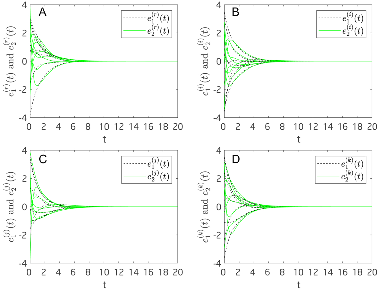
According to the case 3 in Theorem 1, the settling time is estimated as $$ T_{0}=8.4 $$ s. Choosing 8 initial values, Figure 1 gives the states of system error under controller (39). The system (36) and (38) can realize FTS in $$ T_{0} $$ via control scheme (39).

Projective synchronization analysis of multiple-time-scale competitive neural networks in quaternion field

Figure 1. (MatLab) Error states of system (36) and (38) in Simulation 1. (A-D) represents the real and imaginary parts of error state.

Next, we focus on Theorem 2.

Example 2 Consider the QVMTSCNNs (36) and (38). The PTS controller is designed as:

$$ \begin{align} u_{m}(t)=&-\frac{z_{m}(t)}{\|z_{m}(t)\|_{2}+\hat{\sigma}}\Big(S_{m}+\sum\limits_{k=1}^{2}\xi_{mk}\|z_{k}(t-\tau_{k})\|_{2}+X_{m}\varphi(t)\|z_{m}(t)\|_{2}\Big)\\ v_{m}(t)=&-\frac{\varepsilon_{m}(t)}{\|\varepsilon_{m}(t)\|_{2}+\hat{\sigma}}\Big(Q_{m}+Y_{m}\varphi(t)\|\varepsilon_{m}(t)\|_{2}\Big) \end{align} $$

Choose $$ S_{1}=S_{2}=7, \xi_{11}=0.7, \xi_{12}=0.7, \xi_{21}=0.8, \xi_{22}=0.8, X_{1}=X_{2}=1, Q_{1}=Q_{2}=2, Y_{1}=Y_{2}=1 $$. After calculation, we get $$ l_{12}=0.6 $$, $$ l_{22}=0.6 $$, $$ H_{12}=H_{22}=0.2 $$, $$ M_{12}=M_{22}=1.6 $$, $$ \hat{\sigma}=0.001 $$. The condition in Assumption 2.1 and 2.2 holds. Preset $$ T_{p}=6.4s $$, choose projection coefficient $$ \lambda_{1}=\lambda_{2}=1 $$. It is computed that

$$ S_{m}\geq\sum\limits_{k=1}^{2}(\|a_{mk}\|_{2}+\|b_{mk}\|_{2})(H_{k2}+(1+\|\lambda_{m}\|_{2})M_{k2}), \; \xi_{mk}\geq\|b_{mk}\|_{2}l_{k2}, $$

$$ Q_{m}\geq |\beta_{m}|(H_{m2}+(1+\|\lambda_{m}\|_{2})M_{m2}), \; \varpi<\frac{\hat{p}\hat{\nu}}{T_{p}}, \; \hat{p}\hat{\nu}\geq1, \; m=1, 2 $$

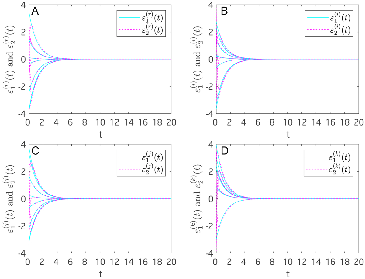
Choose 8 initial values, Figure 2 depicts the states of system error under controller (40). The projective PTS can be realized within $$ T_{p} $$.

Projective synchronization analysis of multiple-time-scale competitive neural networks in quaternion field

Figure 2. (MatLab) Error states of system (36) and (38) in Simulation 2. (A-D) represents the real and imaginary parts of error state.

CONCLUSIONS

This work established the model of QVMTSCNNs for the first time and investigates the projective synchronization problem of this network via non-separation method. Considering the effect of time delays and discontinuous activations, novel controllers are designed without decomposing the quaternion system. Based on nonsmooth analysis and quaternion inequality technique, concise criteria for quaternion projective FTS and PTS of QVMTSCNNs are derived, the convergence time can be adjusted according to task requirement. Furthermore, the proposed control method is designed through algebraic conditions, which is easy to implement. Lastly, simulations are given to verify the results.

DECLARATIONS

Authors' contribution

The conception and design of the work: Wei, R.

Performed data analysis and interpretation: Wu, Y.; Chen, Z.

Provided administrative, technical, and material support: Cao, J.

All authors revised the manuscript.

Availability of data and materials

The data supporting the findings of this study are presented in this manuscript.

AI and AI-assisted tools statement

Not applicable.

Financial support and sponsorship

This work is sponsored by National Natural Science Foundation of China (No. 12301625).

Conflict of interest

Cao, J. is the Editor-in-Chief of the Intelligent Control Systems journal. He had no involvement in the review or editorial process of this manuscript, including but not limited to reviewer selection, evaluation, or the final decision, while the other authors have declared that they have no conflicts of interest.

Ethical approval and consent to participate

Not applicable.

Consent for publication

Not applicable.

Copyright

© The Author(s) 2026.

REFERENCES

1. Meyer-Base, A.; Ohl, F.; Scheich, H. Singular perturbation analysis of competitive neural networks with different time scales. Neural. Comput. 1996, 8, 1731-42.

2. Li, Y.; Yang, X.; Shi, L. Finite-time synchronization for competitive neural networks with mixed delays and non-identical perturbations. Neurocomputing 2016, 185, 242-53.

3. Zou, Y.; Yang, X.; Tang, R.; Cheng, Z. Finite-time quantized synchronization of coupled discontinuous competitive neural networks with proportional delay and impulsive effects. J. Frankl. Inst. 2020, 357, 11136-52.

4. Shi, Y.; Zhu, P. Synchronization of stochastic competitive neural networks with different timescales and reaction-diffusion terms. Neural. Comput. 2014, 26, 2005-24.

5. Gong, S.; Guo, Z.; Wen, S.; Huang, T. Finite-time and fixed-time synchronization of coupled memristive neural networks with time delay. IEEE. Trans. Cybern. 2021, 51, 2944-55.

6. Wang, L.; Zeng, Z.; Ge, M. A disturbance rejection framework for finite-time and fixed-time stabilization of delayed memristive neural networks. IEEE. Trans. Syst. Man. Cybern. Syst. 2021, 51, 905-15.

7. Gao, K.; Lu, J.; Zheng, W. X.; Chen, X. Synchronization in coupled neural networks with hybrid delayed impulses: Average impulsive delay gain method. IEEE. Trans. Neural. Netw. Learning. Syst. 2025, 36, 3608-17.

8. Hamilton, W. R. Lectures quaternions. Dublin, Republic of Ireland: Hodges and Smith; 1853.

9. Took, C.; Mandic, D. The quaternion LMS algorithm for adaptive filtering of hypercomplex processes. IEEE. Trans. Signal. Process. 2009, 57, 1316-27.

10. Zou, C.; Kou, K. I.; Wang, Y. Quaternion collaborative and sparse representation with application to color face recognition. IEEE. Trans. Image. Process. 2016, 25, 3287-302.

11. Xia, Y.; Jahanchahi, C.; Mandic, D. P. Quaternion-valued echo state networks. IEEE. Trans. Neural. Netw. Learning. Syst. 2015, 26, 663-73.

12. Song, Q.; Chen, X. Multistability analysis of quaternion-valued neural networks with time delays. IEEE. Trans. Neural. Netw. Learn. Syst. 2018, 29, 5430-40.

13. Chen, X.; Li, Z.; Song, Q.; Hu, J.; Tan, Y. Robust stability analysis of quaternion-valued neural networks with time delays and parameter uncertainties. Neural. Netw. 2017, 91, 55-65.

14. Liu, Y.; Zheng, Y.; Lu, J.; Cao, J.; Rutkowski, L. Constrained quaternion-variable convex optimization: a quaternion-valued recurrent neural network approach. IEEE. Trans. Neural. Netw. Learn. Syst. 2020, 31, 1022-35.

15. Zhao, Y.; Ren, S.; Kurths, J. Synchronization of coupled memristive competitive BAM neural networks with different time scales. Neurocomputing 2021, 427, 110-7.

16. Yang, W.; Wang, Y.; Morarescu, I.; Liu, X.; Huang, Y. Fixed-time synchronization of competitive neural networks with multiple time scales. IEEE. Trans. Neural. Netw. Learn. Syst. 2022, 33, 4133-8.

17. Liu, P.; Kong, M.; Zeng, Z. Projective synchronization analysis of fractional-order neural networks with mixed time delays. IEEE. Trans. Cybern. 2022, 52, 6798-808.

18. Pu, H.; Li, F.; Wang, Q.; Li, P. Preassigned-time projective synchronization of delayed fully quaternion-valued discontinuous neural networks with parameter uncertainties. Neural. Netw. 2023, 165, 740-54.

19. Wang, S.; Cao, Y.; Wen, S.; Guo, Z.; Huang, T.; Chen, Y. Projective synchroniztion of neural networks via continuous/periodic event-based sampling algorithms. IEEE. Trans. Netw. Sci. Eng. 2020, 7, 2746-54.

20. Bhat, S. P.; Bernstein, D. S. Finite-time stability of continuous autonomous systems. SIAM. J. Control. Optim. 2000, 38, 751-66.

21. Tang, Z.; Park, J. H.; Shen, H. Finite-time cluster synchronization of Lurie networks: a nonsmooth approach. IEEE. Trans. Syst. Man. Cybern. Syst. 2018, 48, 1213-24.

22. Zhang, W.; Yang, X.; Xu, C.; Feng, J.; Li, C. Finite-time synchronization of discontinuous neural networks with delays and mismatched parameters. IEEE. Trans. Neural. Netw. Learning. Syst. 2018, 29, 3761-71.

23. Peng, T.; Zhong, J.; Tu, Z.; Lu, J.; Lou, J. Finite-time synchronization of quaternion-valued neural networks with delays: a switching control method without decomposition. Neural. Netw. 2022, 148, 37-47.

24. Polyakov, A. Nonlinear feedback design for fixed-time stabilization of linear control systems. IEEE. Trans. Automat. Contr. 2012, 57, 2106-10.

25. Chen, C.; Li, L.; Peng, H.; Yang, Y. Fixed-time synchronization of inertial memristor-based neural networks with discrete delay. Neural. Netw. 2019, 109, 81-9.

26. Firouzbahrami, M.; Nobakhti, A. Cooperative fixed-time/finite-time distributed robust optimization of multi-agent systems. Automatica 2022, 142, 110358.

27. Wei, R.; Cao, J.; Kurths, J. Fixed-time output synchronization of coupled reaction-diffusion neural networks with delayed output couplings. IEEE. Trans. Netw. Sci. Eng. 2021, 8, 780-9.

28. Hu, C.; He, H.; Jiang, H. Fixed/preassigned-time synchronization of complex networks via improving fixed-time stability. IEEE. Trans. Cybern. 2021, 51, 2882-92.

29. Hu, C.; Jiang, H. Special functions-based fixed-time estimation and stabilization for dynamic systems. IEEE. Trans. Syst. Man. Cybern. Syst. 2022, 52, 3251-62.

30. Xu, L.; Liu, X. Practical prescribed-time synchronization for multiweighted complex networks. IEEE. Trans. Circuits. Syst. I. 2025, 72, 5119-31.

31. Feng, L.; Yu, J.; Hu, C.; Yang, C.; Jiang, H. Nonseparation method-based finite/fixed-time synchronization of fully complex-valued discontinuous neural networks. IEEE. Trans. Cybern. 2021, 51, 3212-23.

32. Xu, L.; Liu, X. Prescribed-time synchronization of multiweighted and directed complex networks. IEEE. Trans. Automat. Contr. 2023, 68, 8208-15.

33. Liu, X.; Ho, D. W. C.; Xie, C. Prespecified-time cluster synchronization of complex networks via a smooth control approach. IEEE. Trans. Cybern. 2020, 50, 1771-5.

34. Wei, W.; Yu, J.; Wang, L.; Hu, C.; Jiang, H. Fixed/Preassigned-time synchronization of quaternion-valued neural networks via pure power-law control. Neural. Netw. 2022, 146, 341-9.

Cite This Article

Research Article
Open Access
Projective synchronization analysis of multiple-time-scale competitive neural networks in quaternion field

How to Cite

Download Citation

If you have the appropriate software installed, you can download article citation data to the citation manager of your choice. Simply select your manager software from the list below and click on download.

Export Citation File:

Type of Import

Tips on Downloading Citation

This feature enables you to download the bibliographic information (also called citation data, header data, or metadata) for the articles on our site.

Citation Manager File Format

Use the radio buttons to choose how to format the bibliographic data you're harvesting. Several citation manager formats are available, including EndNote and BibTex.

Type of Import

If you have citation management software installed on your computer your Web browser should be able to import metadata directly into your reference database.

Direct Import: When the Direct Import option is selected (the default state), a dialogue box will give you the option to Save or Open the downloaded citation data. Choosing Open will either launch your citation manager or give you a choice of applications with which to use the metadata. The Save option saves the file locally for later use.

Indirect Import: When the Indirect Import option is selected, the metadata is displayed and may be copied and pasted as needed.

About This Article

Disclaimer/Publisher’s Note: All statements, opinions, and data contained in this publication are solely those of the individual author(s) and contributor(s) and do not necessarily reflect those of OAE and/or the editor(s). OAE and/or the editor(s) disclaim any responsibility for harm to persons or property resulting from the use of any ideas, methods, instructions, or products mentioned in the content.
© The Author(s) 2026. Open Access This article is licensed under a Creative Commons Attribution 4.0 International License (https://creativecommons.org/licenses/by/4.0/), which permits unrestricted use, sharing, adaptation, distribution and reproduction in any medium or format, for any purpose, even commercially, as long as you give appropriate credit to the original author(s) and the source, provide a link to the Creative Commons license, and indicate if changes were made.

Data & Comments

Data

Views
21
Downloads
5
Citations
0
Comments
0
0

Comments

Comments must be written in English. Spam, offensive content, impersonation, and private information will not be permitted. If any comment is reported and identified as inappropriate content by OAE staff, the comment will be removed without notice. If you have any queries or need any help, please contact us at [email protected].

0
Download PDF
Share This Article
Scan the QR code for reading!
See Updates
Contents
Figures
Related
Intelligent Control Systems
ISSN : XXXX-XXXX (Coming soon)
Navigation
Navigation