Download PDF
Research Article  |  Open Access  |  25 Mar 2026

Observer-based boundary control for distributed parameter system under denial-of-service attacks

Views: 62 |  Downloads: 0 |  Cited:  0
Complex Eng. Syst. 2026, 6, 5.
10.20517/ces.2025.70 |  © The Author(s) 2026.
Author Information
Article Notes
Cite This Article

Abstract

This paper focuses on the problem of boundary control for a distributed parameter system (DPS) under denial-of-service (DoS) attacks. Initially, a DPS model is employed. Considering the incomplete measurement of the DPS's state, a novel boundary observer is then proposed, which only relies on the right boundary state instead of full-domain information to achieve accurate state estimation, significantly reducing the measurement cost. Subsequently, an anti-DoS observer-based boundary controller is designed, which is applied only to the spatial boundary to lower actuator deployment costs while improving robustness to intermittent DoS attacks. In addition, a Lyapunov-Krasovskii functional is introduced, and the design methods for the controller and observer are derived by solving linear matrix inequalities. Finally, the feasibility of the control strategy is verified through an example.

Keywords

Distributed parameter system, DoS attacks, boundary control

1. INTRODUCTION

Unlike ordinary differential equations (ODEs), partial differential equations (PDEs) can simultaneously capture a system’s temporal and spatial characteristics[1,2,3]. This unique feature allows scholars to delve deeper into nonlinear dynamic phenomena within complex processes, including fluid dynamics[4] and gene regulatory networks[5,6]. As distributed parameter systems (DPSs) are generally modeled by PDEs, their control-related problems have attracted extensive attention from researchers. For complex DPSs, Wang et al.[7] proposed an adaptive spatial model-based predictive controller with real-time linearization. To ensure the exponential stability of the closed-loop parabolic DPS, Wang et al.[8] proposed a fuzzy boundary-based sampled-data control method.

As a widely studied method, the distributed control method needs to be applied to the entire spatial domain, which has excellent control performance but increases the control cost significantly. On the other hand, the boundary control method[9,10] implies that the controller is only imposed on the boundary of the spatial domain. From a cost perspective, the number of actuators is greatly reduced[11], which saves control costs and also decreases the probability of accidents due to machine failures. Moreover, since it is not always feasible to place controllers throughout the entire domain, boundary control not only offers economic benefits but also presents practical advantages when considering spatial constraints on controller placement. Man et al.[10] proposed a boundary control scheme based on the T-S fuzzy model for a nonlinear parabolic PDE system, which effectively satisfies the needs in practical applications. To address the exponential consensus problem of multi-agent systems described by impulsive PDEs, an observer-based event-triggered boundary control strategy was designed in[12], and the Zeno phenomenon was effectively excluded.

Networked control systems often face complex communication constraints, for instance, the authors in[13], in-depth performance analysis of Multiple-Input Multiple-Output (MIMO) time-delay systems under multiple communication parameters and message queue effects. While network transmission offers great efficiency and convenience, cyber-attacks remain a hidden risk. Common types include replay attacks[14,15], deception attacks[16,17], and denial-of-service (DoS) attacks[18,19,20]. DoS attacks, which need no complex techniques, can interrupt data transmission, disable normal network services, and even cause economic losses. Most existing boundary control schemes for DPSs[8,21] ignore cyber-attacks (especially DoS attacks), lacking targeted solutions for DPSs with spatiotemporal dynamics. Furthermore, existing anti-DoS control methods[19,22] rarely combine boundary control with observer design, failing to address the dual challenges of incomplete state measurement and intermittent communication disruptions in DPSs simultaneously. To our knowledge, few studies have focused on the control problem of DPS under DoS attacks.

To fill the gap of lacking anti-DoS boundary control schemes for DPSs with incomplete state measurement, this paper aims to design a cost-effective and robust control protocol. The proposed scheme can handle both practical measurement limitations and intermittent DoS attacks, thereby providing a feasible solution for the safe operation of complex engineering systems modeled by DPSs. Inspired by the above, this paper addresses the problem of anti-DoS observer-based control for DPSs. This paper’s main contributions and novelties are concentrated in the following three points:

(1) Although numerous advancements have been made in DPS control[21,23], there is a noticeable lack of studies exploring control problems under boundary observers. To address the incomplete measurability of the system, this paper introduces a boundary observer based on the right boundary state of DPS.

(2) Traditional observers[24,25] rely on full-domain state information or multiple boundary measurements, leading to high deployment costs. Taking into account the cost issues of distributed control, a boundary controller is proposed that enables it to be applied to the boundary of the spatial domain.

(3) Most existing anti-DoS control studies[19,22] focus on ODE systems, and few target DPSs with spatiotemporal dynamics. Regarding the control problem of DPS, this paper fully considers the impact of DoS attacks, thereby endowing the designed control method with stronger anti-DoS attack performance.

The rest of the paper is structured as follows: Section 2 presents the modeling of DPS, boundary observer, and boundary controller, along with the error system. In Section 3, we give the Lyapunov-Krasovskii functional (LKF), conduct stability analysis, and outline the controller and observer design approach. In Section 4, an example is used to demonstrate the feasibility of the results. Section 5 concludes the article.

Notation: $$ (N + * ) $$ symbolizes $$ (N + {N^T}) $$ and diag$$ \left\{ \cdots \right\} $$ represents a block-diagonal matrix. For a symmetric matrix X, $$ X >0 $$ represents that X is positive definite. Let $$ {\mathcal{H}^n} \buildrel \Delta \over = {\mathcal{L}^2}([{\alpha _1}, {\alpha _2}];{\mathbb{R}^n}) $$ represent the Hilbert space with inner product

$$ \begin{equation*} \langle {{\eta _1}(t, s), {\eta _2}(t, s)} \rangle \buildrel \Delta \over = \int_\Omega {{{\langle {{\eta _1}(t, s), {\eta _2}(t, s)} \rangle }_{{\mathbb{R}^n}}}ds} \\ \end{equation*} $$

and $$ {\left\| {{\eta _i}(t, s)} \right\|_2} \buildrel \Delta \over = {\langle {{\eta _i}(t, s), {\eta _i}(t, s)} \rangle ^{\frac{1}{2}}} $$ with $$ {\eta _1}(t, s), {\eta _2}(t, s) \in {\mathcal H^n} $$. For any integer l, set $$ \langle l \rangle = \left\{ {1, 2, ..., l} \right\} $$.

2. PROBLEM FORMULATION AND PRELIMINARIES

2.1. System description and problem formulation

Consider the following DPS

$$ \begin{equation} \begin{aligned}\left\{ \begin{array}{l}\frac{{\partial v(x, t)}}{{\partial t}} = \Theta \frac{{{\partial ^2}v(x, t)}}{{\partial {x^2}}} + {A_1}v(x, t), \\v(x, 0) = {v_0}(x), \; {v_{out}}(t) = v({\alpha _2}, t), \\\frac{{\partial v(x, t)}}{{\partial x}}{|_{x = {\alpha _1}}} = 0, \; \frac{{\partial v(x, t)}}{{\partial x}}{|_{x = {\alpha _2}}} = u(t), \end{array} \right.\end{aligned} \end{equation} $$

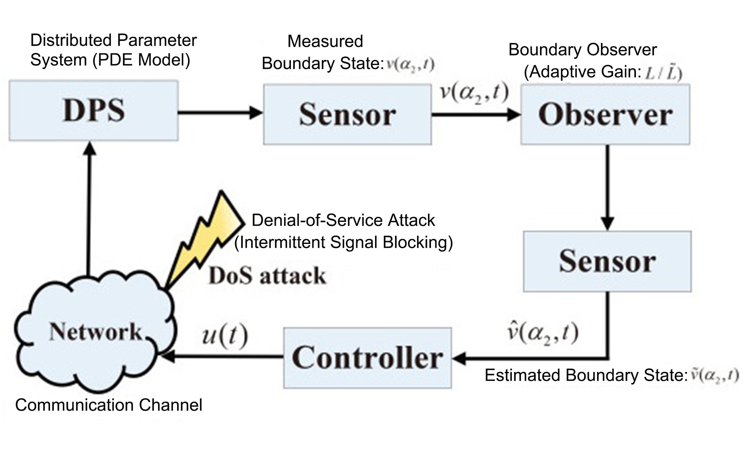
where $$ t \in [0, \infty ) $$ and $$ x \in \Omega \buildrel \Delta \over = [{\alpha _1}, {\alpha _2}] \subset \mathbb R $$ denote the time and space, respectively. $$ v(x, t) \in {\mathbb{R}^{{n_s}}} $$ is the state of the system, $$ u(t) \in {\mathbb{R}^{{n_u}}} $$ is control input. $$ \Theta > 0 \in {\mathbb{R}^{{n_s} \times {n_s}}} $$, $$ {A_1} \in {\mathbb{R}^{{n_s} \times {n_s}}} $$ and $$ B \in {\mathbb{R}^{{n_s} \times {n_u}}} $$ are known constant matrices with appropriate dimensions. The initial condition is represented as $$ {v_0}(x) $$. Considering factors including cost saving and ease of application in complex systems, the observer and controller in this paper are mainly designed through the state information at $$ x = {\alpha _2} $$ (the right boundary of the system and the observer), based on which we set $$ {v_{out}}(t) = v({\alpha _2}, t) $$.

2.2. DoS attacks

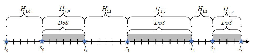
DoS attacks aim to intermittently disrupt communication channels as indicated in[22,26]. Such attacks have particularly notable impacts on the controller, rendering it challenging to control the DPS Equation (1).

The model of DoS attacks is expressed as follows:

$$ \begin{equation} {D_{DoS}} = \left\{ \begin{array}{l}0, \; t \in [{l_n}, {s_n}), \\1, \; t \in [{s_n}, {l_{n + 1}}), \end{array} \right. \end{equation} $$

with time series $$ {\{ {l_n}\} _{n \in \mathbb{N}}} $$ and $$ {\{ {s_n}\} _{n \in \mathbb{N}}} $$ satisfy $$ 0 = {l_0} < {s_0} \le {l_1} < \cdots < {l_n} < {s_n} \le \cdots $$ for $$ {n \in \mathbb{N}} $$.

Take the n-th interval as an example. The interval $$ [{l_n}, {s_n}) $$ indicates that the channel is not blocked and data can be transmitted, and $$ [{s_n}, {l_{n + 1}}) $$ represents that the channel is blocked.

For $$ t \ge {t_r} \ge 0 $$, $$ n({t_r}, t) $$ means the cumulative number of DoS attacks start and stop status changes during the period from $$ {t_r} $$ to t. Additionally, $$ {{\bar \Phi }_{DoS}}({t_r}, t) $$ indicates the collection of durations for which the attacks were active over the interval $$ [{t_r}, t) $$. Based on the above discussion, during $$ [{t_r}, t) $$, the attack sleep interval is

$$ \begin{equation*} {{\bar \Phi }_{sleep}}({t_r}, t) = ({t_r}, t)/{{\bar \Phi }_{DoS}}({t_r}, t). \end{equation*} $$

The framework of DoS attacks is shown in Figure 1. To facilitate the analysis of DoS attacks, the following assumptions are formulated:

Observer-based boundary control for distributed parameter system under denial-of-service attacks

Figure 1. The framework of DoS attacks.

Assumption 1. (DoS Duration) Suppose an interval $$ 0 \le {t_z} \le t $$ and set $$ {T_{D1}} > 0 $$. Then we can get

$$ \begin{equation*} {{\bar \Phi }_{DoS}}({t_r}, t) \le \frac{t}{{{T_{D1}}}}. \end{equation*} $$

2.3. Boundary observer description and problem formulation

In real-world applications, acquiring complete domain state information for Equation (1) is usually unavailable due to limitations such as high measurement cost. Therefore, a boundary state observer is constructed to estimate the state of Equation (1), and subsequently an anti-DoS observer-based controller is designed to achieve effective control for Equation (1).

Taking into account practical factors, this paper assumes that only the state information at $$ x = {\alpha _2} $$ (right boundary of the system) is available, then we set

$$ \begin{equation} \left\{ \begin{array}{l}\frac{{\partial \hat v(x, t)}}{{\partial t}} = \Theta \frac{{{\partial ^2}\hat v(x, t)}}{{\partial {x^2}}} + {A_2}\hat v(x, t) + L({v_{out}}(t) - {{\hat v}_{out}}(t)), \\\hat v(x, 0) = {{\hat v}_0}(x), \; {{\hat v}_{out}}(t) = \hat v({\alpha _2}, t), \\\frac{{\partial \hat v(x, t)}}{{\partial x}}{|_{x = {\alpha _1}}} = 0, \; \frac{{\partial \hat v(x, t)}}{{\partial x}}{|_{x = {\alpha _2}}} = u(t)\end{array} \right. \end{equation} $$

where {$$ \hat v(x, t) \in {\mathbb{R}^{{n_s}}} $$ denotes the observer state. The observer initial condition is given as $$ {{\hat v}_0}(x) $$. The output of the observer is $$ {{\hat v}_{out}}(t) \buildrel \Delta \over = \hat v({\alpha _2}, t) $$. $$ {A_2} \in {\mathbb{R}^{{n_s} \times {n_s}}} $$ is known matrix. $$ L \in {\mathbb{R}^{{n_s} \times {n_s}}} $$ is the boundary observer gain.

Considering the DoS attacks, the observation gain L is expressed in:

$$ \begin{equation*} L = \left\{ \begin{array}{l}L, \; t \in {H_{1, n}}, \\\tilde L, \; t \in {H_{2, n}}, \end{array} \right. \end{equation*} $$

where $$ \tilde L \in {\mathbb{R}^{{n_s} \times {n_s}}} $$ represents the controller gain under DoS attacks.

The aim of this paper is to design an anti-DoS observer-based controller. First, we set a piecewise function $$ p(t) $$

$$ \begin{equation*} p(t) = \left\{ \begin{array}{l}1, \; t \in {H_{1, n}}, \\2, \; t \in {H_{2, n}}, \end{array} \right. \end{equation*} $$

then we can get the feasible set of $$ p(t) $$: $$ {S_p}({\varsigma _{11}}, {\varsigma _{12}};{\varsigma _{21}}, {\varsigma _{22}}) = \{ p(t):{\varsigma _{11}} \le {s_n} - {l_n} \le {\varsigma _{12}};{\varsigma _{21}} \le {l_{n + 1}} - {s_n} \le {\varsigma _{22}}\} $$, {in which $$ {\varsigma _{ij}} > 0 $$, $$ i, j \in \langle 2 \rangle $$ are constants.

Drawing upon the above discussions, the controller is proposed:

$$ \begin{equation} u(t) = \left\{ \begin{array}{l}BK{{\hat v}_{out}}(t), \; t \in {H_{1, n}}, \\0, \; t \in {H_{2, n}}.\end{array} \right. \end{equation} $$

with $$ {B} \in {\mathbb{R}^{{n_s} \times {n_s}}} $$ is known matrix, $$ K \in {\mathbb{R}^{{n_s} \times {n_s}}} $$ is the controller gain.

The estimation error is specified as

$$ e(x, t) \triangleq v(x, t)-\hat{v}(x, t).$$

Based on (5), we have

$$ \begin{equation*} \begin{aligned}\frac{{\partial e(x, t)}}{{\partial t}} =& \frac{{\partial v(x, t)}}{{\partial t}} - \frac{{\partial \hat v(x, t)}}{{\partial t}}\\=& \Theta (\frac{{{\partial ^2}v(x, t)}}{{\partial {x^2}}} - \frac{{{\partial ^2}\hat v(x, t)}}{{\partial {x^2}}}) + {A_1}v(x, t) - {A_2}\hat v(x, t) - L({v_{out}}(t) - {{\hat v}_{out}}(t))\\=& \Theta \frac{{{\partial ^2}e(x, t)}}{{\partial {x^2}}} + {A_1}v(x, t) + {A_2}v(x, t) - {A_2}v(x, t) - {A_2}\hat v(x, t) - L({v_{out}}(t) - {{\hat v}_{out}}(t))\\=& \Theta \frac{{{\partial ^2}e(x, t)}}{{\partial {x^2}}} + ({A_1} - {A_2})v(x, t) + {A_2}e(x, t) - L({v_{out}}(t) - {{\hat v}_{out}}(t)). \end{aligned} \end{equation*} $$

Then, we derive the subsequent error system

$$ \begin{equation} \left\{ \begin{array}{l}\frac{{\partial e(x, t)}}{{\partial t}} = \Theta \frac{{{\partial ^2}e(x, t)}}{{\partial {x^2}}} + {A_2}e(x, t) + ({A_1} - {A_2})v(x, t) - L({v_{out}}(t) - {{\hat v}_{out}}(t)), \\{\left. {\frac{{\partial e(x, t)}}{{\partial x}}} \right|_{x = {\alpha _1}}} = {\left. {\frac{{\partial e(x, t)}}{{\partial x}}} \right|_{x = {\alpha _2}}} = 0, \\e(x, 0) = {e_0}(x), \end{array} \right. \end{equation} $$

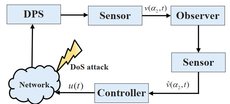
The overall control framework is illustrated in Figure 2. This paper aims to develop an anti-DoS observer-based controller Equation (4), such that the DPS Equation (1) is exponentially stable. For the convenience of stability analysis, the following lemma is presented.

Observer-based boundary control for distributed parameter system under denial-of-service attacks

Figure 2. Observer-based boundary control scheme for DPS under DoS attacks.

Lemma 1. (Wirtinger’s Inequality[21])Set $$ z \in {\mathbb{R}^{{n_s}}} $$ with $$ z({\alpha _2}) = 0 $$ or $$ z({\alpha _1}) = 0 $$. If there exists any matrix $$ U \ge 0 $$, the following inequality is satisfied

$$ \begin{equation*} \int_\Omega {{z^T}} (x)Uz(x)dx \le \frac{{4{{({\alpha _2} - {\alpha _1})}^2}}}{{{\pi ^2}}}\int_\Omega {\frac{{d{z^T}}}{{dx}}U\frac{{dz}}{{dx}}dx} . \end{equation*} $$

In addition, if $$ z({\alpha _2}) = 0 $$ and $$ z({\alpha _1}) = 0 $$, we can deduce that

$$ \begin{equation*} \int_\Omega {{z^T}} (x)Uz(x)dx \le \frac{{{{({\alpha _2} - {\alpha _1})}^2}}}{{{\pi ^2}}}\int_\Omega {\frac{{d{z^T}}}{{dx}}U\frac{{dz}}{{dx}}dx} . \end{equation*} $$

3. MAIN RESULTS

In this part, the design of observers and controllers for DPSs Equations (1) is analyzed and derived based on sufficient conditions obtained from LKF.

Inspired from[27], as for $$ n \in \mathbb{N} $$, the following piecewise linear functions are defined to support the subsequent stability analysis.

$$ \begin{equation*} \begin{aligned}\begin{array}{l}{\theta _{11}}(t) = \frac{{t - {l_n}}}{{{s_n} - {l_n}}}, \; {\theta _{12}}(t) = \frac{{{s_n} - t}}{{{s_n} - {l_n}}}, {\theta _{10}}(t) = \frac{1}{{{s_n} - {l_n}}}, \; t \in {H_{1, n}}, \\{\theta _{21}}(t) = \frac{{t - {s_n}}}{{{l_{n + 1}} - {s_n}}}, {\theta _{22}}(t) = \frac{{{l_{n + 1}} - t}}{{{l_{n + 1}} - {s_n}}}, \; {\theta _{20}}(t) = \frac{1}{{{l_{n + 1}} - {s_n}}}, \; t \in {H_{2, n}}.\end{array}\end{aligned} \end{equation*} $$

Moreover, we can obtain

$$ \begin{equation} \begin{aligned}\begin{array}{l}{\theta _{11}}({l_n}) = {\theta _{22}}(l_n^ - ) = 0, \; {\theta _{11}}(s_n^ - ) = {\theta _{22}}({s_n}) = 1, \\{\theta _{12}}({l_n}) = {\theta _{21}}(l_n^ - ) = 1, \; {\theta _{12}}(s_n^ - ) = {\theta _{21}}({s_n}) = 0.\end{array}\end{aligned} \end{equation} $$

Obviously, there are constants $$ {\varsigma _{ij}} > 0 $$, $$ i, j \in \langle 2 \rangle $$ such that $$ {s_n} - {l_n} \in [{\varsigma _{11}}, {\varsigma _{12}}] $$, $$ {l_{n + 1}} - {s_n} \in [{\varsigma _{21}}, {\varsigma _{22}}] $$ and we can deduce that $$ {\phi _{h1}}(t):{\mathbb{R}_ + } \to [0, 1] $$, satisfy

$$ \begin{equation} \begin{aligned}\begin{array}{l}{\theta _{h0}}(t) = \frac{{{\phi _{h1}}(t)}}{{{\varsigma _{h1}}}} + \frac{{{\phi _{h2}}(t)}}{{{\varsigma _{h2}}}}, \\{\phi _{h2}}(t) = 1 - {\phi _{h1}}(t), \end{array}\end{aligned} \end{equation} $$

with $$ h \in \langle 2 \rangle $$.

Subsequently, the design of controller Equations (4) and observer Equations (3) will be analyzed.

Theorem 1. For given constants $$ {\alpha _1} > 0 $$, $$ {\mu _1} > 1 $$ and $$ {\mu _2} > 1 $$, the control gain K, the observer gain L, if there exist matrices $$ {P_{lm}} \in {\mathbb{R}^{{n_s} \times {n_s}}} > 0 $$, $$ l, m \in \langle 2 \rangle $$, such that

$$ \begin{equation} {P_{22}} \le {\mu _1}{P_{11}}, \; {P_{12}} \le {\mu _2}{P_{21}}, \end{equation} $$

$$ \begin{equation} \Xi _1^m < 0, \end{equation} $$

$$ \begin{equation} \Xi _2^m < 0, \end{equation} $$

$$ \begin{equation} \frac{{\ln {\mu _1}}}{{{\varsigma _{12}}}} - {\alpha _1} > 0, \; \frac{{\ln {\mu _2}}}{{{\varsigma _{22}}}} - {\alpha _1} < 0, \end{equation} $$

$$ \begin{equation} - (\frac{{\ln {\mu _1}}}{{{\varsigma _{1l}}}} - {\alpha _1})(1 - \frac{1}{{{T_{D1}}}}) - (\frac{{\ln {\mu _2}}}{{{\varsigma _{2l}}}} - {\alpha _1})\frac{1}{{{T_{D1}}}} < 0, \; l \in \langle 2 \rangle \end{equation} $$

where

$$ \begin{align*} \Xi _1^{ml} = \left[ {\begin{array}{*{20}{c}}{\Delta _{11}^{ml}}&{\Delta _{12}^m}&{\Delta _{13}^m}&{\Delta _{14}^m}\\* &{\Delta _{22}^m}&{\Delta _{23}^m}&{\Delta _{24}^m}\\* & * &{\Delta _{33}^{ml}}&{\Delta _{34}^m}\\* & * & * &{\Delta _{44}^m}\end{array}} \right], \\\Xi _2^{ml} = \left[ {\begin{array}{*{20}{c}}{\Lambda _{11}^{ml}}&{\Lambda _{12}^m}&{\Lambda _{13}^m}&{\Lambda _{14}^m}\\* &{\Lambda _{22}^m}&{\Lambda _{23}^m}&{\Lambda _{24}^m}\\* & * &{\Lambda _{33}^{ml}}&{\Lambda _{34}^m}\\* & * & * &{\Lambda _{44}^m}\end{array}} \right], \end{align*} $$

$$ \Delta _{11}^m = {\alpha _1}{P_{1m}} + \frac{1}{{{\varsigma _{1l}}}}({P_{11}} - {P_{12}}) + ({P_{1m}}{A_2} + * ) - \frac{{{\pi ^2}}}{{4{{({\alpha _2} - {\alpha _1})}^2}}}({P_{1m}}\Theta + * ) $$, $$ \Delta _{12}^m = \frac{{{\pi ^2}}}{{4{{({\alpha _2} - {\alpha _1})}^2}}}({P_{1m}}\Theta + * ) $$, $$ \Delta _{13}^m = {({P_{1m}}({A_1} - {A_2}))^T} $$, $$ \Delta _{14}^m = {P_{1m}}L $$, $$ \Delta _{22}^m = \frac{2}{{{\alpha _2} - {\alpha _1}}}{P_{1m}}BK - \frac{{{\pi ^2}}}{{4{{({\alpha _2} - {\alpha _1})}^2}}}({P_{1m}}\Theta + * ) $$, $$ \Delta _{33}^m = {\alpha _1}{P_{1m}} + \frac{1}{{{\varsigma _{1l}}}}({P_{11}} - {P_{12}}) + ({P_{1m}}{A_2} + * ) + ({P_{1m}}({A_1} - {A_2}) + * ) - \frac{{{\pi ^2}}}{{4{{({\alpha _2} - {\alpha _1})}^2}}}({P_{1m}}\Theta + * ) $$, $$ \Delta _{34}^m = - {P_{1m}}L + \frac{{{\pi ^2}}}{{4{{({\alpha _2} - {\alpha _1})}^2}}}({P_{1m}}\Theta + * ) $$, $$ \Delta _{44}^m = - \frac{{{\pi ^2}}}{{4{{({\alpha _2} - {\alpha _1})}^2}}}({P_{1m}}\Theta + * ) $$, $$ \Lambda _{11}^m = {\alpha _1}{P_{2m}} + \frac{1}{{{\varsigma _{2l}}}}({P_{21}} - {P_{22}}) + ({P_{2m}}{A_2} + * ) - \frac{{{\pi ^2}}}{{4{{({\alpha _2} - {\alpha _1})}^2}}}({P_{2m}}\Theta + * ) $$, $$ \Lambda _{12}^m = \frac{{{\pi ^2}}}{{4{{({\alpha _2} - {\alpha _1})}^2}}}({P_{2m}}\Theta + * ) $$, $$ \Lambda _{13}^m = {({P_{2m}}({A_1} - {A_2}))^T} $$, $$ \Lambda _{14}^m = {P_{2m}}\tilde L $$, $$ \Lambda _{22}^m = - \frac{{{\pi ^2}}}{{4{{({\alpha _2} - {\alpha _1})}^2}}}({P_{2m}}\Theta + * ) $$, $$ \Lambda _{33}^m = {\alpha _1}{P_{2m}} + \frac{1}{{{\varsigma _{2l}}}}({P_{21}} - {P_{22}}) + ({P_{2m}}{A_2} + * ) + ({P_{2m}}({A_1} - {A_2}) + * ) - \frac{{{\pi ^2}}}{{4{{({\alpha _2} - {\alpha _1})}^2}}}({P_{2m}}\Theta + * ) $$, $$ \Lambda _{34}^m = - {P_{2m}}\tilde L + \frac{{{\pi ^2}}}{{4{{({\alpha _2} - {\alpha _1})}^2}}}({P_{2m}}\Theta + * ) $$, $$ \Lambda _{44}^m = - \frac{{{\pi ^2}}}{{4{{({\alpha _2} - {\alpha _1})}^2}}}({P_{2m}}\Theta + * ) $$, the part of Δ and Λ that are not specified are zero. Then, the DPS Equations (1) and the error system Equations (6) are exponentially stable.

Proof. Replacing $$ {P_{1m}} $$, $$ {P_{2m}} $$, $$ \frac{1}{{{\varsigma _{1l}}}} $$ and $$ \frac{1}{{{\varsigma _{2l}}}} $$ in Equations (10) and (11) by $$ {P_1}(t) $$, $$ {P_2}(t) $$, $$ {\theta _{10}}(t) $$ and $$ {\theta _{20}}(t) $$ we have

$$ \begin{equation} \Xi _1^{}(t) = \left[ {\begin{array}{*{20}{c}}{\Delta _{11}^{}(t)}&{\Delta _{12}^{}(t)}&{\Delta _{13}^{}(t)}&{\Delta _{14}^{}(t)}\\* &{\Delta _{22}^{}(t)}&{\Delta _{23}^{}(t)}&{\Delta _{24}^{}(t)}\\* & * &{\Delta _{33}^{}(t)}&{\Delta _{34}^{}(t)}\\* & * & * &{\Delta _{44}^{}(t)}\end{array}} \right], \end{equation} $$

$$ \begin{equation} \Xi _2^{}(t) = \left[ {\begin{array}{*{20}{c}}{\Lambda _{11}^{}(t)}&{\Lambda _{12}^{}(t)}&{\Lambda _{13}^{}(t)}&{\Lambda _{14}^{}(t)}\\* &{\Lambda _{22}^{}(t)}&{\Lambda _{23}^{}(t)}&{\Lambda _{24}^{}(t)}\\* & * &{\Lambda _{33}^{}(t)}&{\Lambda _{34}^{}(t)}\\* & * & * &{\Lambda _{44}^{}(t)}\end{array}} \right], \end{equation} $$

with $$ {P_{p(t)}}(t) = \sum\limits_{d = 1}^2 {{\theta _{p(t), d}}(t)} {P_{p(t), d}} $$.

Construct the Lyapunov functional as

$$ \begin{equation} {V_{p(t)}}(t) = \sum\limits_{s = 1}^2 {{V_{p(t), s}}(t)} , \end{equation} $$

where

$$ {V_{p(t), 1}}(t) = {\psi _{p(t)}}(t)\int_\Omega {{{\hat v}^T}} (s, t){P_{p(t)}}(t)\hat v(s, t)ds, $$

$$ {V_{p(t), 2}}(t) = {\psi _{p(t)}}(t)\int_\Omega {{e^T}} (s, t){P_{p(t)}}(t)e(s, t)ds, $$

and $$ {\psi _{p(t)}}(t) = \mu _{p(t)}^{{\theta _{p(t), 1}}(t)} $$.

For $$ t \in [{l_n}, {s_n}) $$, $$ p(t) = 1 $$, we can deduce that

$$ \begin{equation*} \begin{aligned}{V_{11}}(t) = {\psi _1}(t)\int_\Omega {{{\hat v}^T}(x, t){P_1}(t)\hat v(x, t)} dx, \\{V_{12}}(t) = {\psi _1}(t)\int_\Omega {{e^T}(x, t){P_1}(t)e(x, t)} dx, \end{aligned} \end{equation*} $$

then we obtain the derivative of $$ {V_{11}}(t) $$ as:

$$ \begin{equation} \begin{aligned}\frac{{\partial {V_{11}}(t)}}{{\partial t}} =& \frac{{\ln {\mu _1}}}{{{s_n} - {l_n}}}{V_{11}}(t) - {\alpha _1}{V_{11}}(t)+ {\psi _1}(t)\int_\Omega {{{\hat v}^T}(x, t){\alpha _1}{P_1}(t)\hat v(x, t)} dx\\&+ {\psi _1}(t)\int_\Omega {{{\hat v}^T}(x, t){\theta _{10}}(t)({P_{11}} - {P_{12}})\hat v(x, t)} dx+ 2{\psi _1}(t)\int_\Omega {{{\hat v}^T}(x, t){P_1}(t)\frac{{\partial \hat v(x, t)}}{{\partial t}}} dx.\end{aligned} \end{equation} $$

Based on Equations (3) and (19), we have

$$ \begin{equation} \begin{aligned}&2{\psi _1}(t)\int_\Omega {{{\hat v}^T}(x, t){P_1}(t)\frac{{\partial \hat v(x, t)}}{{\partial t}}} dx\\=& 2{\psi _1}(t)\int_\Omega {{{\hat v}^T}(x, t){P_1}(t)(\Theta \frac{{{\partial ^2}\hat v(x, t)}}{{\partial {x^2}}}} + {A_2}\hat v(x, t) + Le({\alpha _2}, t))dx\\=& 2{\psi _1}(t)\int_\Omega {{{\hat v}^T}(x, t){P_1}(t)\Theta \frac{{{\partial ^2}\hat v(x, t)}}{{\partial {x^2}}}} dx + 2{\psi _1}(t)\int_\Omega {{{\hat v}^T}(x, t){P_1}(t){A_2}\hat v(x, t)} dx\\&+ 2{\psi _1}(t)\int_\Omega {{{\hat v}^T}(t, s){P_1}(t)L{e_0}({\alpha _2}, t)} dx, \end{aligned} \end{equation} $$

Furthermore, we can get

$$ \begin{equation} \begin{array}{l}2{\psi _1}(t)\int_\Omega {{{\hat v}^T}(x, t){P_1}(t)\Theta \frac{{{\partial ^2}\hat v(x, t)}}{{\partial {x^2}}}} dx\\= \left. {2{\psi _1}(t){{\hat v}^T}(x, t){P_1}(t)\Theta \frac{{\partial \hat v(x, t)}}{{\partial x}}} \right|_{{\alpha _1}}^{{\alpha _2}} - 2{\psi _1}(t)\int_\Omega {\frac{{\partial {{\hat v}^T}(x, t)}}{{\partial x}}{P_1}(t)\Theta \frac{{\partial \hat v(x, t)}}{{\partial x}}} dx\\= 2{\psi _1}(t){{\hat v}^T}({\alpha _2}, t){P_1}(t)\Theta {\left. {\frac{{\partial \hat v(x, t)}}{{\partial x}}} \right|_{{\alpha _2}}} - 2{\psi _1}(t)\int_\Omega {\frac{{\partial {{\hat v}^T}(x, t)}}{{\partial x}}{P_1}(t)\Theta \frac{{\partial \hat v(x, t)}}{{\partial x}}} dx\\= 2{\psi _1}(t){{\hat v}^T}({\alpha _2}, t){P_1}(t)\Theta BK\hat v({\alpha _2}, t) - 2{\psi _1}(t)\int_\Omega {\frac{{\partial {{\hat v}^T}(x, t)}}{{\partial x}}{P_1}(t)\Theta \frac{{\partial \hat v(x, t)}}{{\partial x}}} dx.\end{array} \end{equation} $$

From Lemma 1, we can conclude that

$$ \begin{equation} \begin{aligned}&2{\psi _1}(t)\int_\Omega {\frac{{\partial {{\hat v}^T}(x, t)}}{{\partial x}}{P_1}(t)\Theta \frac{{\partial \hat v(x, t)}}{{\partial x}}} dx\\\le& - {\psi _1}(t)\frac{{{\pi ^2}}}{{4({\alpha _2} - {\alpha _1})}}\int_\Omega {{{(\hat v(x, t) - \hat v({\alpha _2}, t))}^T}({P_1}(t)\Theta + {{({P_1}(t)\Theta )}^T})(\hat v(x, t) - \hat v({\alpha _2}, t))} dx.\end{aligned} \end{equation} $$

Then, from the derivative of $$ {{V_{12}}(t)} $$, we can deduce that

$$ \begin{equation} \begin{aligned}\frac{{\partial {V_{12}}(t)}}{{\partial t}} =& \frac{{\ln {\mu _1}}}{{{s_n} - {l_n}}}{V_{12}}(t) - {\alpha _1}{V_{12}}(t) + {\psi _1}(t)\int_\Omega {{e^T}(x, t){\alpha _1}{P_1}(t)e(x, t)} dx\\&+ {\psi _1}(t)\int_\Omega {{e^T}(x, t){\theta _{10}}(t)({P_{11}} - {P_{12}})e(x, t)} dx + 2{\psi _1}(t)\int_\Omega {{e^T}(x, t){P_1}(t)\frac{{\partial e(x, t)}}{{\partial t}}} dx, \end{aligned} \end{equation} $$

in which

$$ \begin{equation} \begin{aligned}&2{\psi _1}(t)\int_\Omega {{e^T}(x, t){P_1}(t)\frac{{\partial e(x, t)}}{{\partial t}}} dx\\=& 2{\psi _1}(t)\int_\Omega {{e^T}(x, t){P_1}(t)} \{ \Theta \frac{{{\partial ^2}e(x, t)}}{{\partial {x^2}}} + {A_2}e(x, t) + ({A_1} - {A_2})v(x, t) - Le({\alpha _2}, t)\} dx\\=& 2{\psi _1}(t)\int_\Omega {{e^T}(x, t){P_1}(t)} \Theta \frac{{{\partial ^2}e(x, t)}}{{\partial {x^2}}}dx + 2{\psi _1}(t)\int_\Omega {{e^T}(x, t){P_1}(t)} {A_2}e(x, t)dx\\&+ 2{\psi _1}(t)\int_\Omega {{e^T}(x, t){P_1}(t)} ({A_1} - {A_2})(e(x, t) + \hat v(x, t))dx - 2{\psi _1}(t)\int_\Omega {{e^T}(x, t){P_1}(t)} Le({\alpha _2}, t)dx.\end{aligned} \end{equation} $$

Similar to Equations (21) and (22), one has

$$ \begin{equation} \begin{aligned}&{\psi _1}(t)\int_\Omega {{e^T}(x, t){P_1}(t)} \Theta \frac{{{\partial ^2}e(x, t)}}{{\partial {x^2}}}dx\\\le& - {\psi _1}(t)\frac{{{\pi ^2}}}{{4({\alpha _2} - {\alpha _1})}}\int_\Omega {{{(e(x, t) - e({\alpha _2}, t))}^T}({P_1}(t)\Theta + {{({P_1}(t)\Theta )}^T})(e(x, t) - e({\alpha _2}, t))} dx.\end{aligned} \end{equation} $$

Combining Equations (19)-(25), we obtain the following inequality

$$ \begin{equation} \begin{aligned}\frac{{\partial {V_1}(t)}}{{\partial t}} = {\psi _1}(t)\int_\Omega {\varepsilon _1^T} {\Xi _1}(t){\varepsilon _1}dx + (\frac{{\ln {\mu _1}}}{{{s_n} - {l_n}}} - {\alpha _1}){V_1}(t), \end{aligned} \end{equation} $$

with $$ {\varepsilon _1} = {\rm{col}}(\hat v(x, t), \hat v({\alpha _2}, t), e(x, t), e({\alpha _2}, t)) $$.

From Equations (10) and (14), one can derive that

$$ \begin{equation} \begin{aligned}\frac{{\partial {V_1}(t)}}{{\partial t}} \le (\frac{{\ln {\mu _1}}}{{{s_n} - {l_n}}} - {\alpha _1}){V_1}(t), \end{aligned} \end{equation} $$

where $$ {\beta _1} = \frac{{\ln {\mu _1}}}{{{s_n} - {l_n}}} - {\alpha _1} > 0 $$, due to Equation (7), we can easily deduce that

$$ \begin{equation} \begin{aligned}{V_1}(t) \le {e^{ - {\beta _1}(t - {l_n})}}{V_1}({l_n}), t \in {H_{1, n}}.\end{aligned} \end{equation} $$

For $$ t \in [{s_{n}}, {l_{n+1}}) $$, $$ p(t) = 2 $$, we can deduce that

$$ \begin{equation} \begin{aligned}{V_{21}}(t) = {\psi _2}(t)\int_\Omega {{{\hat v}^T}(x, t){P_2}(t)\hat v(x, t)} dx, \\{V_{22}}(t) = {\psi _2}(t)\int_\Omega {{e^T}(x, t){P_2}(t)e(x, t)} dx.\end{aligned} \end{equation} $$

Taking the derivative of $$ {{V_{21}}(t)} $$, we can deduce that:

$$ \begin{equation} \begin{aligned}\frac{{\partial {V_{21}}(t)}}{{\partial t}} =& \frac{{\ln {\mu _2}}}{{{l_{n + 1}} - {s_n}}}{V_{21}}(t) - {\alpha _1}{V_{21}}(t) + {\psi _2}(t)\int_\Omega {{{\hat v}^T}(x, t){\alpha _1}{P_2}(t)\hat v(x, t)} dx\\&+ {\psi _2}(t)\int_\Omega {{{\hat v}^T}(x, t){\theta _{20}}(t)({P_{21}} - {P_{22}})\hat v(x, t)} dx + 2{\psi _2}(t)\int_\Omega {{{\hat v}^T}(x, t){P_2}(t)\frac{{\partial \hat v(x, t)}}{{\partial t}}} dx.\end{aligned} \end{equation} $$

Furthermore, it is obvious that

$$ \begin{equation} \begin{aligned}&2{\psi _2}(t)\int_\Omega {{{\hat v}^T}(x, t){P_2}(t)\frac{{\partial \hat v(x, t)}}{{\partial t}}} dx\\=& 2{\psi _2}(t)\int_\Omega {{{\hat v}^T}(x, t){P_2}(t)\Theta \frac{{{\partial ^2}\hat v(x, t)}}{{\partial {x^2}}}} dx + 2{\psi _2}(t)\int_\Omega {{{\hat v}^T}(x, t){P_2}(t){A_2}\hat v(x, t)} dx\\&+ 2{\psi _2}(t)\int_\Omega {{{\hat v}^T}(x, t){P_2}(t)Le({\alpha _2}, t)} dx, \end{aligned} \end{equation} $$

Similar to Equation (21), it is evident that

$$ \begin{equation} \begin{aligned}&2{\psi _2}(t)\int_\Omega {{{\hat v}^T}(x, t){P_2}(t)\Theta \frac{{{\partial ^2}\hat v(x, t)}}{{\partial {x^2}}}} dx\\=& \left. {2{\psi _2}(t){{\hat v}^T}(x, t){P_2}(t)\Theta \frac{{\partial \hat v(x, t)}}{{\partial x}}} \right|_{{\alpha _1}}^{{\alpha _2}} - 2{\psi _2}(t)\int_\Omega {\frac{{\partial {{\hat v}^T}(x, t)}}{{\partial x}}{P_2}(t)\Theta \frac{{\partial \hat v(x, t)}}{{\partial x}}} dx\\=& - 2{\psi _2}(t)\int_\Omega {\frac{{\partial {{\hat v}^T}(x, t)}}{{\partial x}}{P_2}(t)\Theta \frac{{\partial \hat v(x, t)}}{{\partial x}}} dx\\\le& - {\psi _2}(t)\frac{{{\pi ^2}}}{{4({\alpha _2} - {\alpha _1})}}\int_\Omega {{{(\hat v(x, t) - \hat v({\alpha _2}, t))}^T}({P_2}(t)\Theta + {{({P_2}(t)\Theta )}^T})(\hat v(x, t) - \hat v({\alpha _2}, t))} dx.\end{aligned} \end{equation} $$

For $$ \frac{{\partial {V_{22}}(t)}}{{\partial t}} $$, we get the derivative as

$$ \begin{equation} \begin{aligned}\frac{{\partial {V_{22}}(t)}}{{\partial t}} =& \frac{{\ln {\mu _2}}}{{{l_{n + 1}} - {s_n}}}{V_{22}}(t) - {\alpha _1}{V_{22}}(t) + {\psi _2}(t)\int_\Omega {{e^T}(x, t){\alpha _1}{P_2}(t)e(x, t)} dx\\&+ {\psi _2}(t)\int_\Omega {{e^T}(x, t){\theta _{20}}(t)({P_{21}} - {P_{22}})e(x, t)} dx + 2{\psi _2}(t)\int_\Omega {{e^T}(x, t){P_2}(t)\frac{{\partial e(x, t)}}{{\partial t}}} dx.\end{aligned} \end{equation} $$

Similar to Equation (24), we use the same method and get

$$ \begin{equation} \begin{aligned}&2{\psi _2}(t)\int_\Omega {{e^T}(x, t){P_2}(t)\frac{{\partial e(x, t)}}{{\partial t}}} dx\\=& 2{\psi _2}(t)\int_\Omega {{e^T}(x, t){P_2}(t)} \{ \Theta \frac{{{\partial ^2}e(x, t)}}{{\partial {x^2}}} + {A_2}e(x, t) + ({A_1} - {A_2})(e(x, t) + \hat v(x, t)) - Le({\alpha _2}, t)\} dx\\=& 2{\psi _2}(t)\int_\Omega {{e^T}(x, t){P_2}(t)} \Theta \frac{{{\partial ^2}e(x, t)}}{{\partial {x^2}}}dx + {\psi _2}(t)\int_\Omega {{e^T}(x, t){P_2}(t)} {A_2}e(x, t)dx\\&+ 2{\psi _2}(t)\int_\Omega {{e^T}(x, t){P_2}(t)} ({A_1} - {A_2})(e(x, t) + \hat v(x, t))dx - 2{\psi _2}(t)\int_\Omega {{e^T}(x, t){P_2}(t)} \tilde Le({\alpha _2}, t)dx, \end{aligned} \end{equation} $$

where

$$ \begin{equation} \begin{aligned}&2{\psi _2}(t)\int_\Omega {{e^T}(x, t){P_2}(t)} \Theta \frac{{{\partial ^2}e(x, t)}}{{\partial {x^2}}}dx\\\le& - {\psi _2}(t)\frac{{{\pi ^2}}}{{4({\alpha _2} - {\alpha _1})}}\int_\Omega {{{(e(x, t) - e({\alpha _2}, t))}^T}({P_2}(t)\Theta + {{({P_2}(t)\Theta )}^T})(e(x, t) - e({\alpha _2}, t))} dx.\end{aligned} \end{equation} $$

From Equations (30)-(35), it follows that

$$ \begin{equation} \begin{aligned}\frac{{\partial {V_2}(t)}}{{\partial t}} = {\psi _2}(t)\int_\Omega {\varepsilon _2^T} {\Xi _2}(t){\varepsilon _2}dx + (\frac{{\ln {\mu _2}}}{{{l_{n + 1}} - {s_n}}} - {\alpha _1}){V_2}(t), \end{aligned} \end{equation} $$

where $$ {\varepsilon _2} = {\rm{col}}(\hat v(x, t), \hat v({\alpha _2}, t), e(x, t), e({\alpha _2}, t)) $$.

One can derive from Equations (11) and (15) that

$$ \begin{equation} \begin{aligned}\frac{{\partial {V_2}(t)}}{{\partial t}} \le {\beta _2}{V_2}(t), \end{aligned} \end{equation} $$

with $$ {\beta _2} = \frac{{\ln {\mu _2}}}{{{l_{n + 1}} - {s_n}}} - {\alpha _1} < 0 $$. From Equation (7), which means that

$$ \begin{equation} \begin{aligned}{V_2}(t) \le {e^{ - {\beta _2}(t - {s_n})}}{V_2}({s_n}), \; t \in {H_{2, n}}.\end{aligned} \end{equation} $$

By combining Equations (28) and (38), it can be deduced that the conditions in Equations (7) and (9)–(12) ensure the feasibility of the following inequalities:

$$ \begin{equation} \left\{ \begin{array}{l}{V_2}({s_n}) \le {V_1}(s_n^ - ), \\{V_1}({l_n}) \le {V_2}(l_n^ - ).\end{array} \right. \end{equation} $$

In summary, we can conclude that

$$ \begin{equation} \begin{aligned}V(t) &\le {e^{ - {\beta _1}(t - \frac{t}{{{T_D}}}) - {\beta _2}\frac{t}{{{T_D}}}}}{V_1}(0)\\&= {e^{{\theta _0}t}}{V_1}(0), \end{aligned} \end{equation} $$

in which $$ {\theta _0} = - {\beta _1}(1 - \frac{1}{{{T_{D1}}}}) - {\beta _2}\frac{1}{{{T_{D1}}}} < 0 $$.

It can be concluded that system Equation (1) and the error system Equation (6) are exponentially stable, thereby finishing the proof.

Next, we would like to elaborate on the design methods of boundary controller Equation (4) and observer Equation (3) using Theorem 2. First, we set

$$ \begin{equation} \begin{aligned}&{X_{11}} \buildrel \Delta \over = P_{11}^{ - 1}, \; {X_{21}} \buildrel \Delta \over = P_{21}^{ - 1}, \\&{P_{12}} = {\chi _1}{P_{11}}, \; {P_{22}} = {\chi _2}{P_{21}}, \end{aligned} \end{equation} $$

where $$ {\chi _1} $$, $$ {\chi _2}>0 $$ are constants.

Theorem 2. Consider constants $$ {\alpha _1} > 0 $$, $$ {\chi _l} >0 $$ and $$ {\mu _l} > 1 $$, if there exist matrices $$ {X_{l1}} \in {\mathbb{R}^{{n_s} \times {n_s}}} > 0 $$, $$ l, m \in \langle 2 \rangle $$, such that the following linear matrix inequalities (LMIs) hold:

$$ \begin{equation} {X_{11}} \le {\mu _1}\chi _2^{ - 1}{X_{21}}, \; {X_{21}} \le {\mu _2}\chi _1^{ - 1}{X_{11}}, \end{equation} $$

$$ \begin{equation} \bar \Xi _1^{ml} < 0, \end{equation} $$

$$ \begin{equation} \bar \Xi _2^{ml} < 0, \end{equation} $$

where

$$ \begin{align*} \bar \Xi _1^{ml} = \left[ {\begin{array}{*{20}{c}}{\bar \Delta _{11}^{ml}}&{\bar \Delta _{12}^m}&{\bar \Delta _{13}^m}&{\bar \Delta _{14}^m}\\* &{\bar \Delta _{22}^m}&{\bar \Delta _{23}^m}&{\bar \Delta _{24}^m}\\* & * &{\bar \Delta _{33}^{ml}}&{\bar \Delta _{34}^m}\\* & * & * &{\bar \Delta _{44}^m}\end{array}} \right], \\\bar \Xi _2^{ml} = \left[ {\begin{array}{*{20}{c}}{\bar \Lambda _{11}^{ml}}&{\bar \Lambda _{12}^m}&{\bar \Lambda _{13}^m}&{\bar \Lambda _{14}^m}\\* &{\bar \Lambda _{22}^m}&{\bar \Lambda _{23}^m}&{\bar \Lambda _{24}^m}\\* & * &{\bar \Lambda _{33}^{ml}}&{\bar \Lambda _{34}^m}\\* & * & * &{\bar \Lambda _{44}^m}\end{array}} \right], \end{align*} $$

$$ \bar \Delta _{11}^{ml} = {\alpha _1}\chi _1^{m - 1}{X_{11}} + \frac{1}{{{\varsigma _{1l}}}}({X_{11}} - {\chi _1}{X_{11}}) + (\chi _1^{m - 1}{A_2}{X_{11}} + * ) - \frac{{{\pi ^2}}}{{4{{({\alpha _2} - {\alpha _1})}^2}}}(\chi _1^{m - 1}\Theta {X_{11}} + * ) $$, $$ \bar \Delta _{12}^m = \frac{{{\pi ^2}}}{{4{{({\alpha _2} - {\alpha _1})}^2}}}(\chi _1^{m - 1}\Theta {X_{11}} + * ) $$, $$ \bar \Delta _{13}^m = {(\chi _1^{m - 1}({A_1} - {A_2}){X_{11}})^T} $$, $$ \bar \Delta _{14}^m = \chi _1^{m - 1}{{\bar L}_{11}} $$, $$ \bar \Delta _{22}^m = \frac{2}{{{\alpha _2} - {\alpha _1}}}\chi _1^{m - 1}B{{\bar K}_{11}} - \frac{{{\pi ^2}}}{{4{{({\alpha _2} - {\alpha _1})}^2}}}(\chi _1^{m - 1}\Theta {X_{11}} + * ) $$, $$ \bar \Delta _{33}^{ml} = {\alpha _1}\chi _1^{m - 1}{X_{11}} + \frac{1}{{{\varsigma _{1l}}}}({X_{11}} - {\chi _1}{X_{11}}) + (\chi _1^{m - 1}{A_2}{X_{11}} + * ) + (\chi _1^{m - 1}({A_1} - {A_2}){X_{11}} + * ) - \frac{{{\pi ^2}}}{{4{{({\alpha _2} - {\alpha _1})}^2}}}(\chi _1^{m - 1}\Theta {X_{11}} + * ) $$, $$ \bar \Delta _{34}^m = - \chi _1^{m - 1}{{\bar L}_{11}} + \frac{{{\pi ^2}}}{{4{{({\alpha _2} - {\alpha _1})}^2}}}(\chi _1^{m - 1}\Theta {X_{11}} + * ) $$, $$ \bar \Delta _{44}^m = - \frac{{{\pi ^2}}}{{4{{({\alpha _2} - {\alpha _1})}^2}}}(\chi _1^{m - 1}\Theta {X_{11}} + * ) $$, $$ \bar \Lambda _{11}^{ml} = {\alpha _1}\chi _2^{m - 1}{X_{21}} + \frac{1}{{{\varsigma _{2l}}}}({X_{21}} - {\chi _2}{X_{21}}) + (\chi _2^{m - 1}{A_2}{X_{21}} + * ) - \frac{{{\pi ^2}}}{{4{{({\alpha _2} - {\alpha _1})}^2}}}(\chi _2^{m - 1}\Theta {X_{21}} + * ) $$, $$ \bar \Lambda _{12}^m = \frac{{{\pi ^2}}}{{4{{({\alpha _2} - {\alpha _1})}^2}}}(\chi _2^{m - 1}\Theta {X_{21}} + * ) $$, $$ \bar \Lambda _{13}^m = {(\chi _2^{m - 1}({A_1} - {A_2}){X_{21}})^T} $$, $$ \bar \Lambda _{14}^m = \chi _2^{m - 1}{{\bar L}_{21}} $$, $$ \bar \Lambda _{22}^m = - \frac{{{\pi ^2}}}{{4{{({\alpha _2} - {\alpha _1})}^2}}}(\chi _2^{m - 1}\Theta {X_{21}} + * ) $$, $$ \bar \Lambda _{33}^{ml} = {\alpha _1}\chi _2^{m - 1}{X_{21}} + \frac{1}{{{\varsigma _{2l}}}}({X_{21}} - {\chi _2}{X_{21}}) + (\chi _2^{m - 1}{A_2}{X_{21}} + * ) + (\chi _2^{m - 1}({A_1} - {A_2}){X_{21}} + * ) - \frac{{{\pi ^2}}}{{4{{({\alpha _2} - {\alpha _1})}^2}}}(\chi _2^{m - 1}\Theta {X_{21}} + * ) $$, $$ \bar \Lambda _{34}^m = - \chi _2^{m - 1}{{\bar L}_{21}} + \frac{{{\pi ^2}}}{{4{{({\alpha _2} - {\alpha _1})}^2}}}(\chi _2^{m - 1}\Theta {X_{21}} + * ) $$, $$ \bar \Lambda _{44}^m = - \frac{{{\pi ^2}}}{{4{{({\alpha _2} - {\alpha _1})}^2}}}(\chi _2^{m - 1}\Theta {X_{21}} + * ) $$,

the part of $$ \bar \Delta $$ and $$ \bar \Lambda $$ that are not specified are zero. Moreover, the controller gains are designed as $$ K = {{\bar K}_{11}}X_{11}^{ - 1} $$, and the observer gains $$ L = {{\bar L}_{11}}X_{11}^{ - 1} $$, $$ \tilde L = {{\bar L}_{21}}X_{21}^{ - 1} $$.

Proof. Pre- and post-multiplying Equations (14) and (15) by $$ {\rm{diag}}\{ {X_{11}}, {X_{11}}, {X_{11}}, {X_{11}}\} $$ and $$ {\rm{diag}}\{ {X_{21}}, {X_{21}}, {X_{21}}, {X_{21}}\} $$. Then we complete the proof.

4. NUMERICAL EXAMPLES

In this section, we provide an example to indicate the feasibility of the observer (3) and boundary controller (4). Consider the following DPS:

$$ \begin{equation*} \label{01}\begin{aligned}\left\{ \begin{array}{l}\frac{{\partial v(x, t)}}{{\partial t}} = \Theta \frac{{{\partial ^2}v(x, t)}}{{\partial {x^2}}} + {A_1}v(x, t), \\v(x, 0) = {v_0}(x), \; {v_{out}}(t) = v({\alpha _2}, t), \\\frac{{\partial v(x, t)}}{{\partial x}}{|_{x = {\alpha _1}}} = 0, \; \frac{{\partial v(x, t)}}{{\partial x}}{|_{x = {\alpha _2}}} = u(t), \end{array} \right.\end{aligned} \end{equation*} $$

and following observer:

$$ \begin{equation*} \label{3}\left\{ \begin{array}{l}\frac{{\partial \hat v(x, t)}}{{\partial t}} = \Theta \frac{{{\partial ^2}\hat v(x, t)}}{{\partial {x^2}}} + {A_2}\hat v(x, t) + L({v_{out}}(t) - {{\hat v}_{out}}(t)), \\\hat v(x, 0) = {{\hat v}_0}(x), \; {{\hat v}_{out}}(t) = \hat v({\alpha _2}, t), \\\frac{{\partial \hat v(x, t)}}{{\partial x}}{|_{x = {\alpha _1}}} = 0, \; \frac{{\partial \hat v(x, t)}}{{\partial x}}{|_{x = {\alpha _2}}} = u(t).\end{array} \right. \end{equation*} $$

where $$ v(x, t) = col\{ {v_1}(x, t), {v_2}(x, t), {v_3}(x, t)\} $$, $$ \hat v(x, t) = col\{ {{\hat v}_1}(x, t), {{\hat v}_2}(x, t), {{\hat v}_3}(x, t)\} $$, $$ {\alpha _1} = 0 $$, $$ {\alpha _2} = 5 $$, $$ {A_1} = - 4 \times {I_3} $$, $$ {A_2} = - {I_3} $$, $$ \Theta = {I_3} $$ and $$ B = {I_3} $$.

Subject to initial conditions

$$ \begin{equation*} \left\{ \begin{array}{l}{v_1}(x, 0) = \sin (0.5\pi x), \\{{\hat v}_1}(x, 0) = \cos (0.5\pi x), \end{array} \right.\left\{ \begin{array}{l}{v_2}(x, 0) = \cos (0.5\pi x), \\{{\hat v}_2}(x, 0) = \sin (0.5\pi x), \end{array} \right.\left\{ \begin{array}{l}{v_3}(x, 0) = \cos (0.7\pi x), \\{{\hat v}_3}(x, 0) = \sin (0.8\pi x).\end{array} \right. \end{equation*} $$

We use MATLAB (Matrix Laboratory) to verify that the LMIs presented in Theorem 2 have a feasible solution. Based on the results above, we can derive the corresponding controller gain matrix and observer gain matrices, and the results are as follows:

$$ \begin{align*} K = - 1.5067 \times {I_3}, \; L = 3.6189 \times {I_3}, \; \tilde L = 4.8605 \times {I_3}. \end{align*} $$

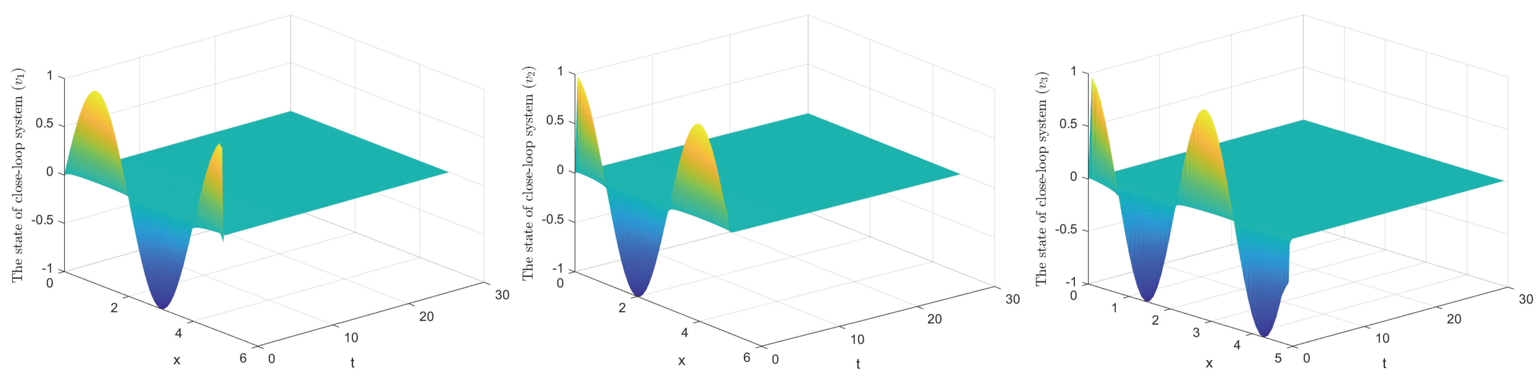
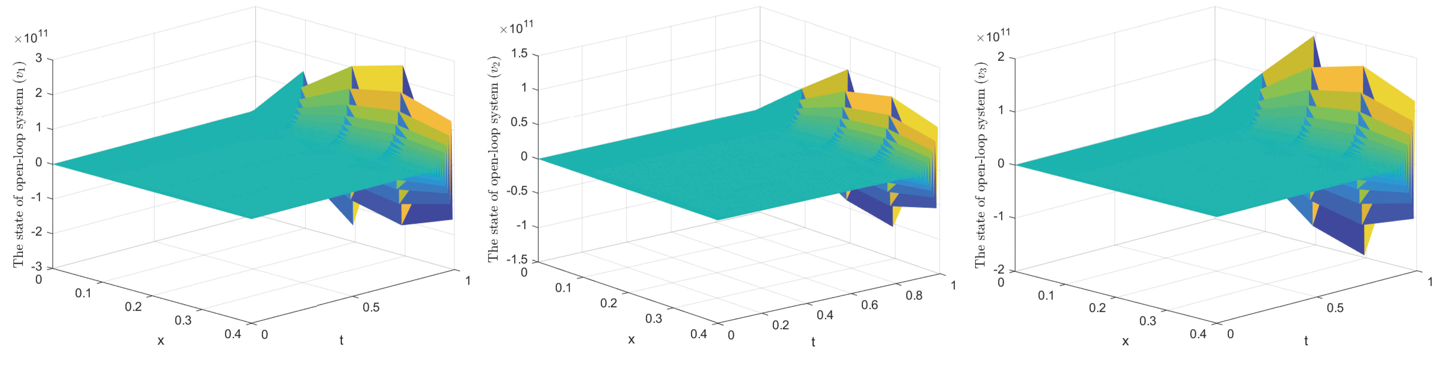
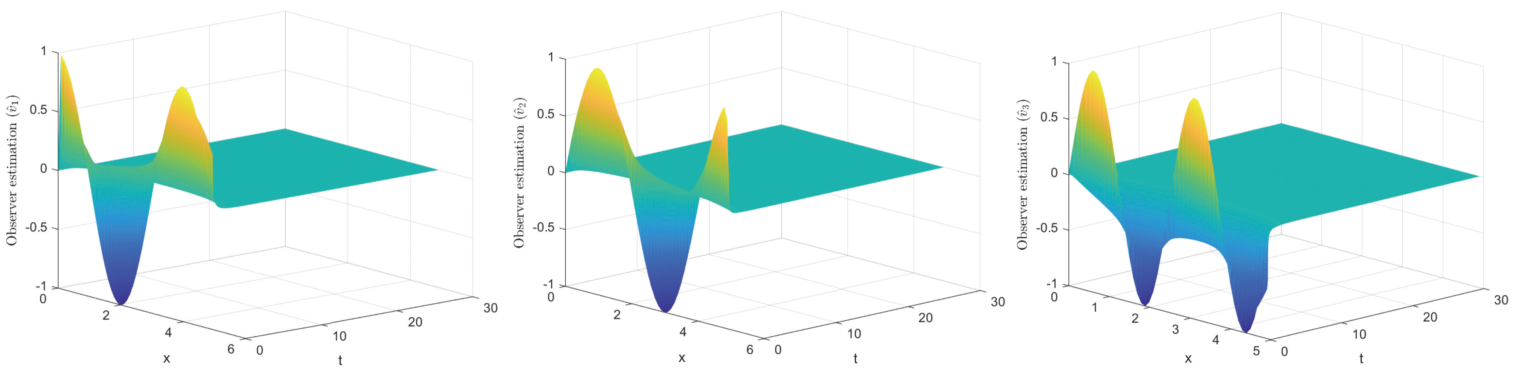
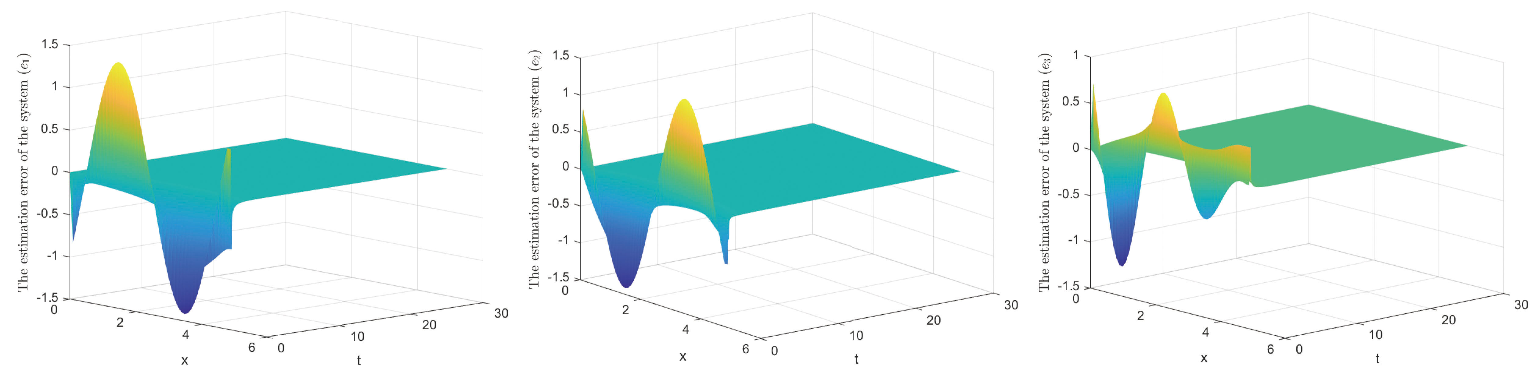
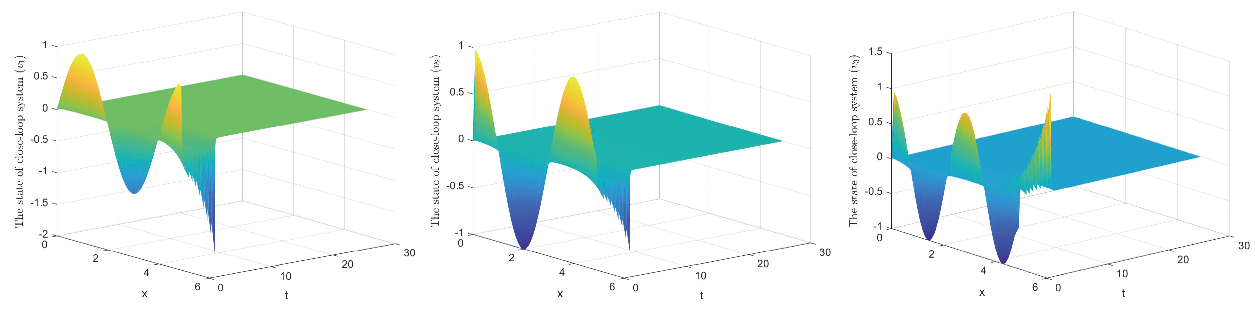
As indicated in Figure 3, the controller drives the system to gradually achieve stability. Conversely, Figure 4 demonstrates that without the controller, the system exhibits divergence over time. The observed state of the system is depicted in Figure 5, and the observation error curve is shown in Figure 6. These results confirm that the observer provides accurate estimates of the system state and transmits this information to the controller, thereby ensuring the effectiveness of the control.

Observer-based boundary control for distributed parameter system under denial-of-service attacks

Figure 3. The state of close-loop system.

Observer-based boundary control for distributed parameter system under denial-of-service attacks

Figure 4. The state of open-loop system.

Observer-based boundary control for distributed parameter system under denial-of-service attacks

Figure 5. Observer state.

Observer-based boundary control for distributed parameter system under denial-of-service attacks

Figure 6. The estimation error of the system.

It is worth noting that most existing studies fail to consider the impact of DoS attacks, and conventional controllers typically rely directly on full system outputs or multi-point boundary measurements for feedback control[28].

In traditional methods, the controller Equation (4) is usually designed as

$$ \begin{equation*} u(t) = {K_0}{v_{out}}(t). \end{equation*} $$

When this controller is used to control the system Equation (1), the matrices and parameters of the system are consistent with those in the above.We ultimately obtain the controller gain $$ {K_0} = -0.7983 \times {I_3} $$.

The state of the closed-loop system obtained thereby is shown in Figure 7. The results demonstrate that although such traditional controllers can maintain the stability of system Equation (1) without considering DoS attacks or incorporating observers, the proposed method in this paper simultaneously integrates the suppression of DoS attack interference and state estimation via observers. It is more aligned with practical engineering scenarios involving communication attacks and constrained state measurement, thus exhibiting more prominent application value.

Observer-based boundary control for distributed parameter system under denial-of-service attacks

Figure 7. System states of the traditional strategy (Without DoS Attacks and Observer).

5. CONCLUSIONS

In this paper, the problem of boundary control for DPSs under DoS attacks has been addressed. First, a PDE-based DPS model has been established to accurately characterize the system’s spatiotemporal dynamics, and a boundary observer dependent only on the right boundary state has been designed to tackle the practical issue of incomplete state measurement in complex DPSs. Then, an anti-DoS observer-based boundary controller has been proposed, which is applied solely to the spatial boundary to reduce actuator deployment costs while ensuring robustness against intermittent DoS attacks. Additionally, a systematic design strategy for the observer and controller gains has been presented by constructing a LKF and solving LMIs, which theoretically guarantees the exponential stability of the closed-loop system. Finally, the feasibility and effectiveness of the proposed method have been fully demonstrated through a numerical example. This strategy not only theoretically guarantees the exponential stability of the closed-loop system but also quantifies the trade-off between attack parameters and system stability performance, thereby filling the gap in quantitative design criteria for anti-DoS control of DPSs.

DECLARATIONS

Authors’ contributions

Methodology, writing - original draft, investigation, conceptualization: Wang, Y.

Conceptualization, investigation, visualization: Zhao, N.

Availability of data and materials

The raw data and experimental datasets supporting this research were generated through numerical simulations based on the proposed theoretical model.

AI and AI-assisted tools statement

Not applicable.

Financial support and sponsorship

None.

Conflicts of interest

Both authors declared that there are no conflicts of interest.

Ethical approval and consent to participate

Not applicable.

Consent for publication

Not applicable.

Copyright

© The Author(s) 2026.

REFERENCES

1. Lu, G.; Zhang, L.; Song, S.; Song, X. Observer-based quantized control for networked interconnected PDE systems with actuator failures. J. Franklin. Inst. 2024, 361, 107208.

2. Guan, Y.; Jiang, B.; Chen, Y. PDE-based fault-tolerant control of swarm deployment while preserving connectedness. J. Franklin. Inst. 2023, 360, 13339-58.

3. Song, X.; Zhang, Q.; Song, S.; Ahn, C. K. Event-triggered underactuated control for networked coupled PDE-ODE systems with singular perturbations. IEEE. Syst. J. 2023, 17, 4474-84.

4. Benner, P.; Hinze, M. Chapter 4 - Feedback control of time-dependent nonlinear PDEs with applications in fluid dynamics. In Handbook of Numerical Analysis, Elsevier, 2023; pp. 77-130.

5. Fan, X.; Xue, Y.; Zhang, X.; Ma, J. Finite-time state observer for delayed reaction-diffusion genetic regulatory networks. Neurocomputing 2017, 227, 18-28.

6. Liu, Q.; Lv, Z.; Zou, C.; Zhang, H. Finite-time stability analysis of interacting genetic regulatory networks with spatial diffusion term. Comput. Biol. Med. 2025, 195, 110585.

7. Wang, Y.; Li, H.; Yang, H. Adaptive spatial-model-based predictive control for complex distributed parameter systems. Adv. Eng. Inform. 2024, 59, 102331.

8. Wang, Z. P.; Li, Q. Q.; Qiao, J.; Wu, H. N.; Huang, T. Fuzzy boundary sampled-data control for nonlinear parabolic DPSs. IEEE. Trans. Cybern. 2024, 54, 3565-76.

9. Wang, P.; Katz, R.; Fridman, E. Constructive finite-dimensional boundary control of stochastic 1D parabolic PDEs. Automatica 2023, 148, 110793.

10. Man, J.; Zeng, Z.; Sheng, Y. Finite-time fuzzy boundary control for 2-D spatial nonlinear parabolic PDE systems. IEEE. Trans. Fuzzy. Syst. 2023, 31, 3278-89.

11. Wang, Z.; Zhang, X.; Qiao, J.; Wu, H.; Huang, T. Synchronization of reaction–diffusion neural networks with random time-varying delay via intermittent boundary control. Neurocomputing 2023, 556, 126645.

12. Wang, X.; Wu, H.; Cao, J.; Li, X. Dynamic event-triggered boundary control for exponential consensus of multi-agent systems of impulsive PDEs with switching topology. Inform. Sci. 2024, 655, 119901.

13. Zhan, X.; Du, X.; Wu, J.; Yan, H. Performance analysis of MIMO Information time-delay systems with message queue under multiple communication parameters. IEEE. Trans. Syst. Man. Cybern. Syst. 2024, 54, 88-96.

14. Zhu, G.; Xu, Z.; Gao, Y.; Yu, Y.; Li, L. Periodic event-triggered adaptive neural output feedback tracking control of unmanned surface vehicles under replay attacks. Eng. Appl. Artif. Intel. 2025, 146, 110237.

15. Su, L.; Ye, D.; Zhao, X. Static output feedback secure control for cyber-physical systems based on multisensor scheme against replay attacks. Int. J. Robust. Nonlinear. Control. 2020, 30, 8313-26.

16. Li, Y.; Liu, H.; Wang, H.; Lai, Y. Active security control for helicopter systems under targeted deception attacks based on Stackelberg game. J. Franklin. Inst. 2026, 363, 108300.

17. Dai, H.; Guo, X.; Ji, L.; Li, H. Bipartite synchronization of multi-agent systems under deception attacks via pinning delayed-impulsive control. Int. J. Robust. Nonlinear. Control. 2023, 33, 7718-34.

18. Zhang, S.; Yin, X.; Gao, Z. Prescribed-time consensus control of nonlinear time-delayed multi-agent systems under DoS attacks. ISA. Trans. 2025.

19. Wu, X.; Xu, N.; Ding, S.; Zhao, X.; Niu, B.; Wang, W. Event-based adaptive neural resilient formation control for MIMO nonlinear MASs under actuator saturation and denial-of-service attacks. Inform. Sci. 2025, 691, 121619.

20. Wang, S.; Wu, D.; You, Z.; Feng, N.; Mao, M. Event-triggered prescribed performance control for trajectory tracking of unmanned surface vehicle under DoS attacks. Ocean. Eng. 2026, 343, 123451.

21. Wang, Z.; Chen, B.; Qiao, J.; Wu, H.; Huang, T. Fuzzy boundary sampled-data control for nonlinear DPSs with Random time-varying delays. IEEE. Trans. Fuzzy. Syst. 2024, 32, 5872-85.

22. Wan, M.; Xu, Y.; Wu, Z. Dynamic event-triggered resilient control of nonlinear multi-agent systems against asynchronous DoS attacks. IEEE. Trans. Automat. Sci. Eng. 2025, 22, 13633-43.

23. Liu, Y.; Zhang, W.; Wang, J.; Liu, Y.; Peng, J. Event-triggered feedback control for nonlinear parabolic distributed parameter systems with time-varying delays. IEEE. Trans. Automat. Sci. Eng. 2025, 22, 5308-21.

24. Cheng, J.; Tang, T.; Yan, H.; Wu, Z.; Zhang, D. A novel switching rule to observer-based control for switched systems. Automatica 2026, 183, 112622.

25. Farbood, M.; Echreshavi, Z.; Mobayen, S.; Skruch, P. Resilient event-triggered observer-based control of uncertain nonlinear fuzzy systems subject to unknown inputs. IEEE. Access. 2025, 13, 156359-74.

26. Wang, Y.; Zeng, Z.; Liu, X.; Liu, Z. Input-to-state stability of switched linear systems with unstabilizable modes under DoS attacks. Automatica 2022, 146, 110607.

27. Zhao, N.; Zhang, H.; Shi, P. Observer-based sampled-data adaptive tracking control for heterogeneous nonlinear multi-agent systems under denial-of-service attacks. IEEE. Trans. Automat. Sci. Eng. 2025, 22, 4771-9.

28. Wang, Z. P.; Zhang, X.; Wu, H. N.; Huang, T. Fuzzy boundary control for nonlinear delayed DPSs under boundary measurements. IEEE. Trans. Cybern. 2023, 53, 1547-56.

Cite This Article

Research Article
Open Access
Observer-based boundary control for distributed parameter system under denial-of-service attacks

How to Cite

Download Citation

If you have the appropriate software installed, you can download article citation data to the citation manager of your choice. Simply select your manager software from the list below and click on download.

Export Citation File:

Type of Import

Tips on Downloading Citation

This feature enables you to download the bibliographic information (also called citation data, header data, or metadata) for the articles on our site.

Citation Manager File Format

Use the radio buttons to choose how to format the bibliographic data you're harvesting. Several citation manager formats are available, including EndNote and BibTex.

Type of Import

If you have citation management software installed on your computer your Web browser should be able to import metadata directly into your reference database.

Direct Import: When the Direct Import option is selected (the default state), a dialogue box will give you the option to Save or Open the downloaded citation data. Choosing Open will either launch your citation manager or give you a choice of applications with which to use the metadata. The Save option saves the file locally for later use.

Indirect Import: When the Indirect Import option is selected, the metadata is displayed and may be copied and pasted as needed.

About This Article

Disclaimer/Publisher’s Note: All statements, opinions, and data contained in this publication are solely those of the individual author(s) and contributor(s) and do not necessarily reflect those of OAE and/or the editor(s). OAE and/or the editor(s) disclaim any responsibility for harm to persons or property resulting from the use of any ideas, methods, instructions, or products mentioned in the content.
© The Author(s) 2026. Open Access This article is licensed under a Creative Commons Attribution 4.0 International License (https://creativecommons.org/licenses/by/4.0/), which permits unrestricted use, sharing, adaptation, distribution and reproduction in any medium or format, for any purpose, even commercially, as long as you give appropriate credit to the original author(s) and the source, provide a link to the Creative Commons license, and indicate if changes were made.

Data & Comments

Data

Views
62
Downloads
0
Citations
0
Comments
0
0

Comments

Comments must be written in English. Spam, offensive content, impersonation, and private information will not be permitted. If any comment is reported and identified as inappropriate content by OAE staff, the comment will be removed without notice. If you have any queries or need any help, please contact us at [email protected].

0
Download PDF
Share This Article
Scan the QR code for reading!
See Updates
Contents
Figures
Related
Complex Engineering Systems
ISSN 2770-6249 (Online)

Portico

All published articles are preserved here permanently:

https://www.portico.org/publishers/oae/

Portico

All published articles are preserved here permanently:

https://www.portico.org/publishers/oae/