An integrated energy system scheduling method considering year-round load variations based on deep reinforcement learning

Traditional optimization dispatch approaches

In existing research, numerous traditional approaches have been proposed to address the scheduling issues of IES^[6]. Initially, optimization problems for IES relied on traditional linear programming (LP) methods that were simple and easy to implement^[7]. However, with the need to consider discrete and continuous decision problems for each piece of equipment, mixed integer linear programming (MILP) and mixed-integer nonlinear programming (MILNP) in mathematical programming methods are used to handle such optimization problems^[8]. Subsequently, the dynamic programming (DP) method was introduced to handle multi-stage decision problems considering time series, such as optimizing the operation of IES over multiple periods^[9]. As the scale and complexity of optimization problems increase, the above methods face challenges regarding time and space processing. Heuristic and metaheuristic algorithms, represented by the genetic algorithm (GA)^[10], particle swarm optimization (PSO) algorithm^[11], and simulated annealing (SA), are widely used due to their advantages in finding approximate solutions to large-scale problems^[12].

However, the above traditional mathematical models face challenges in solving energy system operation optimization problems, which are characterized by multivariate, multi-constraint, and multi-dimensional features. Due to the introduction of energy storage and renewable energy, the complexity and randomness of the energy system have increased. Therefore, the application of AI algorithms in the energy field is gradually emerging ^[13]. Attributed to its robust nonlinear fitting capabilities, model-agnostic nature, and proficient decision-making process, RL as a kind of AI is proposed to address such operation problems in IES^[14].

RL application in IES optimization dispatch

RL is a decision-based learning method that can learn optimal strategies through interaction with the environment. This ability makes RL suitable for applications that require continuous decision-making, such as the optimization scheduling of IES under the renewable and load uncertainty scenario^[15]. The RL method based on the value function, represented by Q-Learning, is used to learn the value function (Q-value) of long-term expected benefits for taking each possible action under a given state^[16]. However, handling high-dimensional state spaces is difficult because they rely on lookup tables to store the values of each state-action pair, which becomes infeasible when the state or action space is large.

Deep reinforcement learning (DRL) performs outstandingly in tasks with complex or high-dimensional state spaces^[17] in IES. This technology combines deep learning (DL) with RL^[18], utilizing DL models to represent strategies or value functions in RL. According to the characteristics and mechanisms of DRL, it can be divided into value-based methods^[19] and policy-based methods^[20]. Deep Q network (DQN)^[21], double DQN, and double dueling deep Q Net (D3QN) are value-based methods. This approach focuses on learning the value of each state or state-action pair to maximize future expected returns. It is suitable for problems with discrete action spaces, such as starting a device or adjusting power output levels. Zheng et al. used the D3QN method and proposed a multi-stage real-time dispatch method for IES based on RL^[22]. The convergence rate is accelerated by reducing the number of actions in the action space and introducing an improved action-choosing strategy^[4]. However, this method is hardly applicable when the action space is large and continuous. Compared with the value-based method of DRL, policy-based methods represented by REINFORCE, advantage Actor-Critic (A2C), and Asynchronous Advantage Actor-Critic (A3C) can optimize directly in the policy space, handle continuous action spaces, and directly output the optimal action^[23]. Nakabi et al. utilized the A3C algorithm in their study on enhancing the energy management system of a microgrid using DRL^[24]. The methods above cannot address IES optimization problems characterized by continuous control.

The deep deterministic policy gradient (DDPG) excels in handling continuous action spaces and leverages deep neural networks for complex environments. It incorporates experience replay and target networks to stabilize training and improve sample efficiency. Despite the potential slower convergence speed, DDPG remains a potent algorithm for solving challenging RL problems. Yang et al. introduced an enhanced DDPG algorithm to address IES’s dynamic energy dispatch challenge^[25]. Thus, the improved version of DDPG, Twin Delayed DDPG (TD3), is applied to address the continuous control optimization problem of IES operation in this study.

In conclusion, DRL has yielded specific achievements in addressing the optimization challenges of IES operations. It is well-suited for addressing continuous decision-making problems, yet it presents challenges in handling device shutdown actions. Moreover, in scenarios characterized by high-dimensional action and state spaces, establishing the reward function poses significant challenges, as it is pivotal for quantifying objectives and facilitating interaction between IES and algorithms. An improperly set reward function can readily lead to disordered device output, necessitating the inclusion of specific constraints. Consequently, our literature review focuses on the DRL training sets, agents, and reward functions, as shown in Table 1, and we raise the following questions.

(1) For the training set, existing studies predominantly address a single type of load, ranging from a few days to several months, rarely including data for an entire year.

(2) For agent control, the TD3 algorithm can address IES optimization problems involving continuous control. However, the current TD3 agent is commonly used for controlling continuous actions, making it challenging to achieve shutdown actions for devices with discrete action characteristics, such as thermal energy storage system (TESS) and battery energy storage system (BESS) equipment. This results in unreasonable energy storage and other device outputs.

(3) Most studies only consider cost and power constraints for the reward function. Agents have long learning times and slow convergence rates. Furthermore, the limitations in training set length and learning time can lead to insufficient learning by the agents, resulting in improper device operation.

Objective function

The optimization problem aims to minimize the operational expenses of the energy system. Hence, the daily operational cost is the designated objective function, as given in

where COST represents the cost incurred by the IES, and the variable t signifies the time step denoted in h. $$ \operatorname{COST}_{\text {Grid }}^{t} $$ represents the grid cost, while $$ \operatorname{COST}_{\text {PG }}^{t} $$ is the natural gas cost at time step t.

Electricity and natural gas procurement expenditures can be computed by multiplying the consumption by the respective prices using

where $$ \operatorname{E}_{\text {Grid }}^{t} $$ and $$ \operatorname{NG}_{\text {GE }}^{t} $$ symbolize the electricity output and gas quantities, respectively. $$ \operatorname{Pr}_{\text {E }}^{t} $$ and $$ \operatorname{Pr}_{\text {NG }}^{t} $$ represent the prices of electricity and natural gas for the given time step, respectively.

Constraint setting

The constraints primarily encompass limitations on device output concerning performance, along with constraints ensuring energy balance.

(1) Constraints on device performance

The GE must ensure that its electrical and thermal power outputs remain within the specified maximum and minimum generation capacities and the defined maximum and minimum heating capacities.

where $$ \operatorname{E}_{\text {GE }}^{t} $$ and $$ \operatorname{H}_{\text {GE }}^{t} $$ denote the electricity and heat output generated by the GE, respectively. $$ \operatorname{E}_{\text {GE }}^{Min} $$ and $$ \operatorname{E}_{\text {GE }}^{Max} $$ refer to the minimum and maximum electricity generation capacities of the GE. Similarly, $$ \operatorname{H}_{\text {GE }}^{Min} $$ and $$ \operatorname{H}_{\text {GE }}^{Max} $$ represent the minimum and maximum heat generation capacities. The efficiencies of the GE for electricity and heat are denoted by $$ \operatorname{η}_{\text {GE }}^{E} $$ and $$ \operatorname{η}_{\text {GE }}^{H} $$, respectively. $$ \operatorname{NG}_{\text {GE }}^{t} $$ indicates the natural gas consumed by the GE, and LCV stands for the lower calorific value of the natural gas.

The AC utilizes waste heat from the GE and must operate within the defined maximum and minimum cooling power limits.

where $$ \operatorname{C}_{\text {AC }}^{Min} $$ and $$ \operatorname{C}_{\text {AC }}^{Max} $$ denote the minimum and maximum cooling outputs of the AC, respectively. $$ \operatorname{C}_{\text {AC }}^{t} $$ represents the AC’s cooling capacity at time step t. $$ \operatorname{H}_{\text {AC }}^{t} $$ indicates the heat obtained by the AC, and COP_AC refers to the coefficient of performance (COP) of the AC.

The HP uses electrical energy to provide heat and must adhere to its COP and maximum and minimum heating power limits.

where $$ \operatorname{H}_{\text {HP }}^{Min} $$ and $$ \operatorname{H}_{\text {HP }}^{Max} $$ denote the minimum and maximum heating capacities of the HP, the COP_HP represents the COP of the HP. $$ \operatorname{H}_{\text {HP }}^{t} $$ and $$ \operatorname{E}_{\text {HP }}^{t} $$ indicate the heat and electricity generated by the HP at time t, respectively.

The EC uses electrical energy to provide cooling and must comply with its COP and maximum and minimum cooling power limits.

where $$ \operatorname{C}_{\text {EC }}^{Min} $$ and $$ \operatorname{C}_{\text {EC }}^{Max} $$ represent the minimum and maximum cooling outputs from the EC, respectively. $$ \operatorname{C}_{\text {EC }}^{t} $$ and $$ \operatorname{E}_{\text {EC }}^{t} $$ denote the cooling output and electricity consumption of the EC at time step t. The COP_EC represents the COP of the EC.

The BESS manages energy through charging and discharging processes and must adhere to its capacity limits and maximum charging and discharging capabilities.

where $$ \operatorname{SOC}_{\text {BESS }}^{t} $$ represents the state of charge (SOC) of the BESS. $$ \operatorname{SOC}_{\text {BESS }}^{Min} $$ and $$ \operatorname{SOC}_{\text {BESS }}^{Max} $$ denote the minimum and maximum SOC of the BESS, respectively. $$ \operatorname{E}_{\text {BESS }}^{t} $$ indicates the charging or discharging electrical amount of the BESS, Cap_BESS signifies the capacity of the BESS, and $$ \operatorname{η}_{\text {BESS }}^{ch,dis} $$ denotes the efficiency of the BESS during charging and discharging.

The TESS manages energy by storing and releasing heat, and it must adhere to its capacity limits and maximum charging and heat release capabilities.

where $$ \operatorname{SOC}_{\text {TESS }}^{t} $$ represents the SOC of TESS. $$ \operatorname{SOC}_{\text {TESS }}^{Min} $$ and $$ \operatorname{SOC}_{\text {TESS }}^{Max} $$ stand for the minimum and maximum SOC of TESS, respectively. $$ \operatorname{H}_{\text {TESS }}^{t} $$ is the amount of heat charged or discharged by the TESS. $$ \operatorname{H}_{\text {TESS }}^{t} $$ and $$ \operatorname{H}_{\text {TESS }}^{Max} $$ stand for the amount of TESS and the maximum amount of TESS, respectively. Cap_TESS denotes the capacity of the TESS, and $$ \operatorname{η}_{\text {TESS }}^{ch,dis} $$ represents the efficiency of the TESS during charging and discharging.

(2) Constraints of energy balance

The load balancing constraints are established to fulfill user demands, and the constraints for cooling, heating, and electricity loads are expressed as follows:

where $$ \operatorname{E}_{\text {PV }}^{t} $$ represents the electricity generated by PV panels. $$ \operatorname{C}_{\text {d }}^{t} $$, $$ \operatorname{H}_{\text {d }}^{t} $$, and $$ \operatorname{E}_{\text {d }}^{t} $$ denote the cooling, heating, and electric demand at time t, respectively.

State space

The state space denotes the feasible states of the environment observable by the agent. In this study, the states encompass the energy demand at the user side, PV power generation, electricity price, and SOC of the BESS and TESS at each time step t. To delineate the state space, these states above are defined in

where s^t denotes the state space. $$ \operatorname{C}_{\text {d }}^{t} $$, $$ \operatorname{H}_{\text {d }}^{t} $$, and $$ \operatorname{E}_{\text {d }}^{t} $$ represent the cooling, heating, and electric demand at time t, respectively.

Action space

The action space represents the set of all conceivable actions accessible to the agent within the environment. In optimizing the IES, the action space encompasses the decision variables within the agent’s control, comprising the output of the GE and the charging or discharging power of the BESS and TESS. These decision variables are expounded upon in

where a^t denotes the action space. $$ \operatorname{a}_{\text {GE }}^{t} $$, $$ \operatorname{a}_{\text {BESS }}^{t} $$, and $$ \operatorname{a}_{\text {TESS }}^{t} $$ represent the actions of the GE, BESS, and TESS at time t. Since the air conditioner (AC) output is contingent upon the GE, and the EC and HP are solely utilized to meet the cooling and heating load demands, respectively, they remain beyond the realm of control.

Reward function

The reward function is pivotal in RL, guiding the agent toward the desired behavior and optimal policy. In this study, the reward function consists of three primary components:

(1) Operating cost: The cost of purchasing electricity from the grid and natural gas, which the agent seeks to minimize.

(2) Supply-demand balance: Encourages stable and reliable operation of the IES.

(3) Expert knowledge penalties: Incorporate domain-specific constraints and preferences to discourage irrational actions.

While the initial two components of the reward function are consistent across the three agents undergoing training, the third component, expert knowledge, is tailored to accommodate the distinct load characteristics. This approach enables the agents to acquire policies attuned to the various load profiles.

Formulating the reward function is a critical step in guiding the RL algorithm towards the targeted optimization objectives for the IES, as given in

where r^t represents the reward function, α, β, and γ are constants. α, β, and γ are constants used to describe the weights of cost, energy balance, and penalty, respectively. where α, β, and γ are set to 0.0001, 0.0003, and 0.01, respectively. The results are obtained using the optimal system cost through experiments. EB denotes the amount of energy imbalance, encompassing cooling, heating, and electric load. $$ \operatorname{P}_{\text {action }}^{t} $$ represents the penalty for irrational actions.

Validation of load clustering and expert knowledge under Cluster 2

This section compares and analyzes the impact of expert knowledge and clustering on equipment output and system cost. A typical day under heating conditions is selected as the research object. The device output and heat load distribution are depicted in Figure 9. The heat load is supplied by three devices, namely GE, TESS, and HP, with HP’s electrical energy sourced from GE, PV, Grids, and BESS. HP’s output is distributed based on the current output ratios of Grids, PV, GE, and BESS. It is observed that the TD3c2 agent, without prior knowledge, only learned the scheduling strategy for TESS and failed to learn about BESS. This deficiency is evident in Figure 9, where the absence of the green portion compared to other agents indicates BESS did not contribute to the energy dispatch.

Figure 9. The impact of clustering and expert knowledge on the output of different devices. (A) Output of different devices in TD3base scenario; (B) Output of different devices in TD3c2 scenario; (C) Output of different devices in TD3c2-wpk scenario; (D) Output of different devices in MPC scenario. TD3base: This primary scenario does not employ load clustering and does not incorporate expert knowledge into the reward function; TD3c2: scenario with clustering under heating electricity load; TD3c2-wpk: scenario with clustering and expert knowledge under heating electricity load; MPC: operational optimization using model predictive control algorithms; HP: heat pump; BESS: battery electricity energy storage; PV: photovoltaic; GE: gas engine; TESS: thermal energy storage system.

From the output of HP, it is apparent that BESS did not participate in the energy conversion, resulting in a loss of potential profits from lower nighttime electricity prices. This occurred because TESS scheduling was more accessible to optimize for higher rewards, causing the agent to neglect the scheduling strategy for BESS, which might require longer training steps to achieve. From the graph of TD3base, there is no TESS activity after 20 h. This is attributed to both agents maintaining the SOC of TESS at a high level, thereby lacking effective utilization. Additionally, the power generation of GE in TD3base is lower than the others, leading to a failure in harnessing combined heat and power generation.

As shown in Figure 9D, compared with the TD3 method method, the limited control step size of MPC prevents effective use of heat pumps to store thermal energy in the TESS during periods of low electricity prices, reducing potential benefits. Given that RL possesses long-term planning capabilities, the costs of TD3base, TD3c2, and TD3c2-wpk are all lower than those of MPC.

Table 5 summarizes the impact of clustering and expert knowledge on system cost. Compared to the TD3base scenario, the TD3c2 scenario, after clustering, optimized the output of each device and reduced system costs by 9.3%. After incorporating expert knowledge, the learning of TESS and BESS became more effective, and the TD3-wpk scenario further reduced the cost by 2.4% compared to scenario TD3c2. Due to the inability to perform long-term optimization, its operating cost exceeds the optimization results of all RL scenarios.

Validation of CNN utilized under Cluster 3

In the last scenario of a typical day in cluster result 3, the figures utilize device output and electrical load to explain. Since the test set load encompasses cooling, heating, and electricity, and both cooling and heating loads are minimal, the device schedule differs from the first two typical days, as depicted in Figure 10. From 0 to 5 h, TD3c0 (scenarios representing typical electric cooling and heat loads) utilized Grids to store energy in TESS. However, this typical day had no heat load, resulting in energy waste. TD3c0’s action is attributed to the inclusion of current load demand in the state space and the similar nighttime load demands, with only an electrical load. Consequently, TD3c0 could not ascertain the necessity of storing heat. In contrast, the TD3c0-wpk agent, which incorporates expert knowledge and CNN processors for nested agents based on scenarios representing typical electric cooling and heating loads, effectively schedules the BESS under the constraints of CNN on TESS actions and, when trained with prior knowledge, reduces the system cost by 7.58% [Table 6].

Figure 10. Typical day of cluster result in 3 for TD3 with load clustering (A) TD3 with prior knowledge and load clustering (B). TD3: Twin-delayed deep deterministic policy gradient; TD3c0:scenarios representing typical lower-level mixed cooling, heating, and electricity load loads; TD3c0-wpk: incorporates expert knowledge and CNN processors for nested agents based on scenarios representing typical lower-level mixed cooling, heating, and electricity load; PV: photovoltaic; BESS: battery energy storage system; GE: gas engine.

Validation of CNN-MTD3 under cooling scenario

To validate the comprehensive efficacy of the CNN-MTD3 algorithm framework, this study considers that the benefits of energy storage devices may not be fully discernible within a typical day. Therefore, two scenarios are selected, each spanning 120 h, encompassing both the cooling and heating seasons. A comparison is conducted to assess the impact of this study’s proposed CNN-MTD3 and TD3 baseline on device performance.

During the test period, from August 28^th to September 2^nd, emphasis is placed on electricity and cooling load as the primary variables. The data generated by each device exemplifies specific equipment actions, as depicted in Figure 11. Notably, the cooling load registers higher levels during the initial three days. In contrast, the subsequent two days witness a decrease due to the operational cycle of the office building. Throughout the first three days, the cooling load peaks between 9 AM and 12 PM, followed by a gradual decline. Employing the CNN-MTD3 method, the BESS exhausts all its stored electricity to fulfill the demand of the peak cooling load. Conversely, during the last two days, characterized by the reduced loads, the stored electricity in BESS takes approximately 9 to 10 h to discharge completely. In contrast, BESS’s involvement in the TD3base algorithm is comparatively lesser, particularly noticeable on the final day at 7 PM. To utilize the surplus electrical energy stored in BESS, the cooling load is solely supported by the EC, necessitating the shutdown of the GE, thereby impacting GE’s subsequent efficiency.

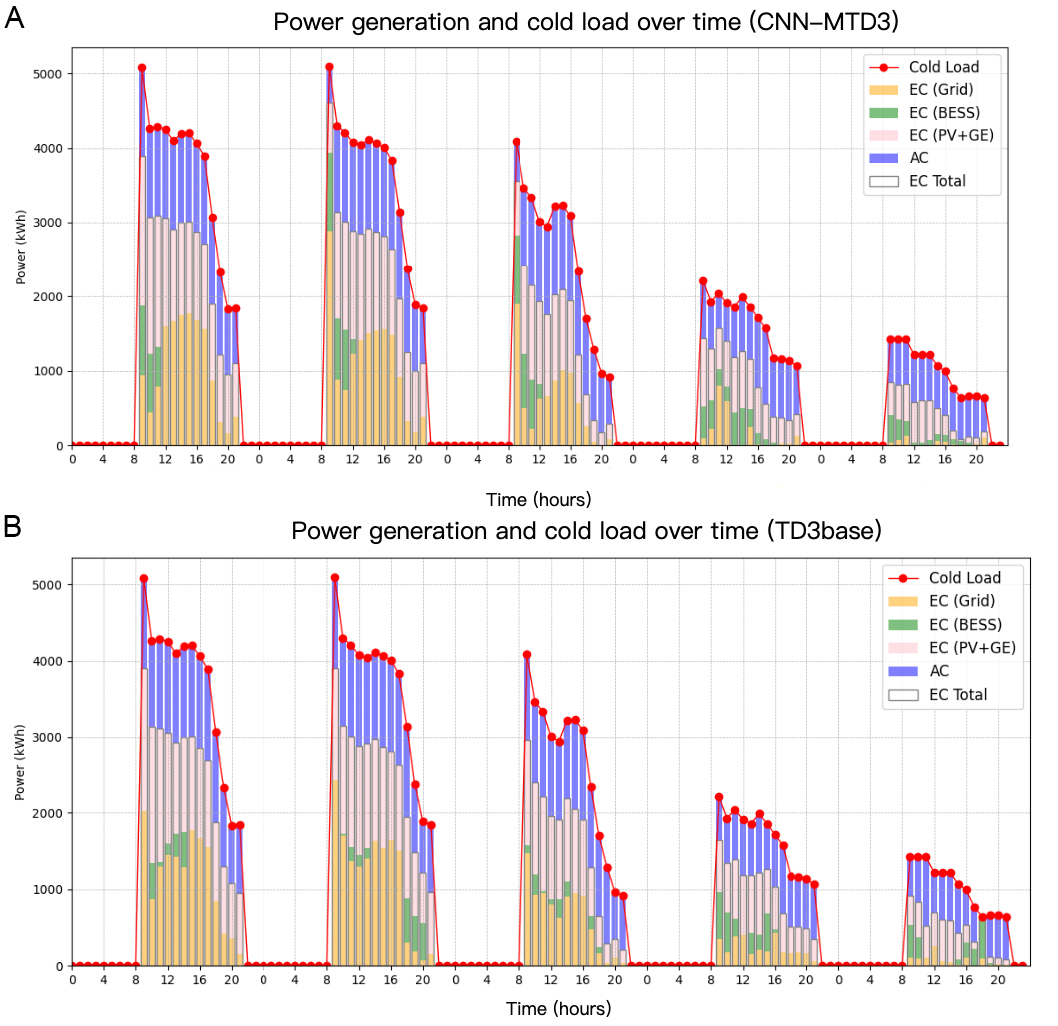
Figure 11. Operation in the cooling scenario for 120 h of CNN-MTD3 (A) and TD3base (B). CNN-MTD3: A deep reinforcement learning algorithm proposed in this paper; CNN: convolutional neural network; MTD3: multi agent of twin delayed deep deterministic policy gradient; EC: electricity cooling; BESS: battery energy storage system; PV: photovoltaic; GE: gas engine; AC: absorption cooling; TD3base: this primary scenario does not employ load clustering and does not incorporate expert knowledge into the reward function.

Validation of CNN-MTD3 under heating scenario

In the second scenario, December 24^th to December 31^st is chosen as the test set, focusing on electricity and heating loads. Figure 12 illustrates that the TD3base algorithm better understands BESS charging and discharging strategies. BESS’s participation is notably higher than that of TESS. Initially, TD3base fully charges TESS, but it struggles to release stored thermal energy effectively in subsequent scheduling. This may be attributed to TD3base being trained on the annual test set, making learning the BESS strategy easier than TESS. Conversely, within the selected five days of the test set, CNN-MTD3 discovers that both TESS and BESS engage in a broader spectrum of energy exchanges. Notably, TESS utilizes GE’s waste heat for energy storage in the 20th hour of each day, exploiting the surplus electricity load without heat demand, thereby effectively leveraging GE’s waste heat and minimizing energy wastage.

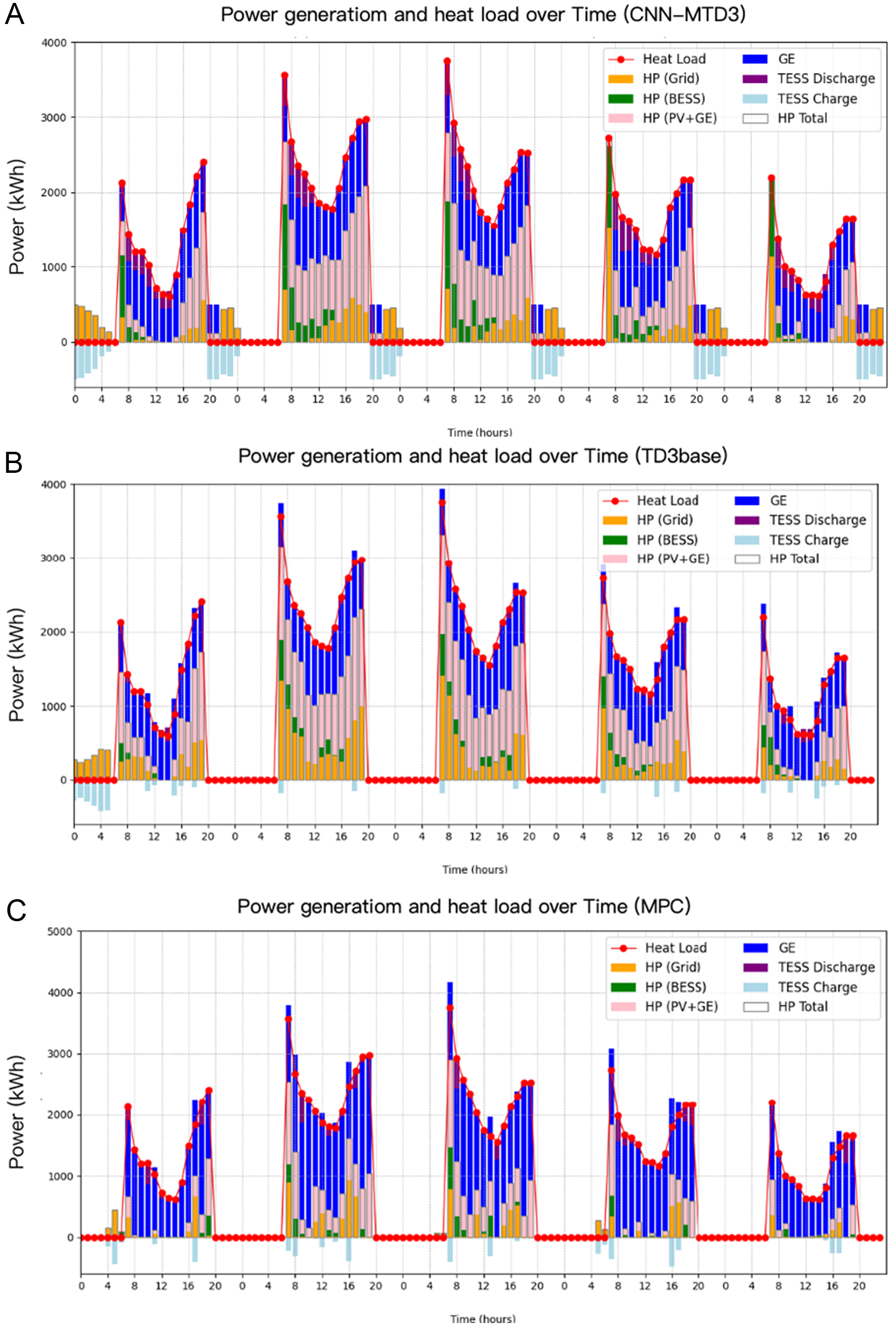
Figure 12. Operation in the heating scenario for 120 h of CNN-MTD3 (A), TD3base (B) and MPC (C). CNN-MTD3: A deep reinforcement learning algorithm proposed in this paper; CNN: convolutional neural network; MTD3: multi agent of twin delayed deep deterministic policy gradient method; TD3base: this primary scenario does not employ load clustering and does not incorporate expert knowledge into the reward function; MPC: operational optimization using model predictive control algorithms; HP: heat pump; BESS: battery electricity energy storage; PV: photovoltaic; GE: gas engine; TESS: thermal energy storage system.

Besides, Figure 12C illustrates a scenario in which MPC was configured for a 120-hour operational optimization. A comparison with TD3base reveals that, under the MPC application, the BESS and TESS were not utilized effectively; energy storage activities continued even during periods when electricity prices were not at off-peak levels, thereby increasing costs.

Performance comparison

This section compares the performance of the TD3base, CNN-MTD3 and MPC models by evaluating the operational cost and effective operating h in different scenarios. As depicted in Table 7, for both cooling and heating scenarios, the cost incurred by the CNN-MTD3 framework is lower than that of the base scenario. Specifically, compared to the base scenario, system costs in the cooling and heating scenarios are reduced by 4.7% and 10.4%, respectively. Furthermore, due to the MPC’s lack of global optimization capabilities, energy storage devices were not utilized to their full potential, resulting in a 9.37% increase in costs compared to the TD3base heating scenario, which operates continuously for 120 h.

Effective operating h refer to the actual number of h that equipment operates within a specific time frame. This metric is crucial as it reflects the stability and reliability of the system. By monitoring the adequate operation time of the equipment, one can evaluate the system’s performance and operational efficiency. An increase in effective operating time indicates higher utilization, thereby leading to a more efficient energy supply and cost reduction. Table 8 presents the operating time for both models in the cooling and heating scenarios, respectively.

The CNN-MTD3 model excels in managing the BESS and AC units for the cooling scenario, as shown in Table 8. It demonstrates an increase in effective operating h by 4.82 and 0.74 h, respectively, compared to the TD3base model. This illustrates the significant advantage of the CNN-MTD3 model in optimizing operational efficiency and control strategies for these devices. Although there is a slight decrease in operating h for the GE and EC devices, the overall difference is minimal, indicating the stable performance of the CNN-MTD3 model with these types of equipment.

For the heating scenario, the CNN-MTD3 model particularly shines with the BESS and TESS devices. As shown in Table 7, it substantially increases the effective operating h by 10.43 and 13.8 h, respectively. This reflects the model’s exceptional ability to manage charging and discharging strategies and the efficiency of energy storage devices. The operating time of the GE equipment increased slightly by 1.62 h. The CNN-MTD3 model primarily achieves a substantial increase in the effective utilization hours of energy storage equipment.

Sensitivity analysis of cluster number

To verify the impact of the number of clusters on system performance optimization, we conducted a sensitivity analysis by varying the number of clusters from 2 to 5. The results are shown in Figure 13A. Excessive clustering increases the probability of misclassification in the CNN algorithm. At the same time, too many clusters reduce the size of the training dataset available for each agent, and misclassification during training also hinders the training of the agents. In addition, we conducted a comparative analysis of the system optimization costs under different numbers of clusters, as shown in Figure 13B. It is worth noting that this analysis is based on a typical heating day, where the agents were deployed in strict accordance with the clustering results. Under these conditions, an increase in the number of clusters was not observed to yield significant cost improvements.

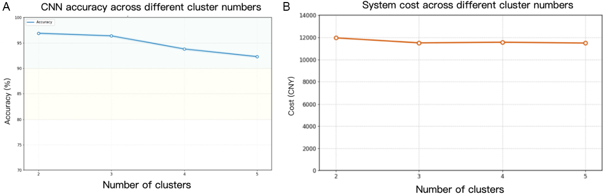
Figure 13. Variation in CNN-based agent classification accuracy (A) and IES cost with different numbers of clusters (B). CNN: Convolutional neural network; IES: integrated energy system.

Sensitivity analysis of CNN performance on agent selection

Throughout the IES operation optimization process in CNN-MTD3, the CNN plays a critical role in load classification and agent selection. To this end, we analyzed the scenarios in which misclassification occurred and their impact on system optimization. Figure 14 displays the loss, accuracy, and start/stop status of TESS for the CNN’s load classification in this study. The loss function exhibits a positive downward trend, indicating stable model training. The CNN classification accuracy exceeds 96%, and the TESS start-stop accuracy is around 95%, indicating that the CNN performs well.

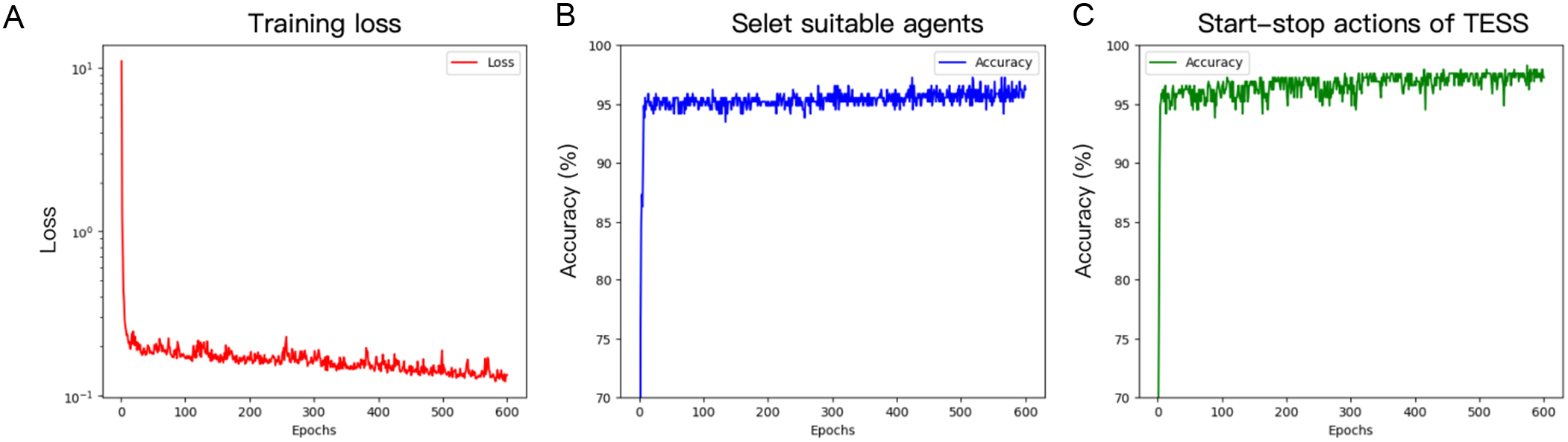
Figure 14. The training process diagram of CNN training loss (A), accuracy of select suitable agents (B), and accuracy of start-stop actions of TESS. CNN: Convolutional neural network; TESS: thermal energy storage system.

Furthermore, Figure 15 shows that, in the 100-day validation dataset, the CNN misclassified on 4 days: days 96, 186, 188, and 329 of the year. In the vast majority of cases, the CNN classifier clearly distinguishes between different scenes (as indicated by the clearly defined blue rectangles). The only four misclassifications (marked by red diamonds) all occurred in the boundary regions between different scene types, representing a typical case of boundary ambiguity rather than a structural failure of the model. The confusion matrix shows the scenarios in which the agents made misclassifications. Agents 1, 2, and 3 made 2, 1, and 1 misclassifications, respectively.

Figure 15. Maximum daily load distribution (A) and confusion matrix (B) for load classification and agent selection on CNN. CNN: Convolutional neural network.

A comparison of the operating costs between the correct and incorrect agents is shown in Table 9. It can be seen that the cost difference is not significant. Compared to the operating cost of the correct agent, the cost under the optimized operation of the incorrect agent increased by a maximum of 2.5%. This is because the similarity of the loads leads to similar decisions by the agents.

REFERENCES

1. Deng, X.; Zhang, Y.; Jiang, Y.; Zhang, Y.; Qi, H. A novel operation method for renewable building by combining distributed DC energy system and deep reinforcement learning. Appl. Energy. 2024, 353, 122188.
2. Mehigan, L.; Deane, J.; Gallachóir, B.; Bertsch, V. A review of the role of distributed generation (DG) in future electricity systems. Energy 2018, 163, 822-36.
3. Liu, R.; He, G.; Su, Y.; Yang, Y.; Ding, D. Solar energy for low carbon buildings: choice of systems for minimal installation area, cost, and environmental impact. City. Built. Enviro. 2023, 1, 16.
4. Shi, L.; Lao, W.; Wu, F.; Lee, K. Y.; Li, Y.; Lin, K. DDPG-based load frequency control for power systems with renewable energy by DFIM pumped storage hydro unit. Renew. Energy. 2023, 218, 119274.
5. Wang, X.; Kang, X.; An, J.; Chen, H.; Yan, D. Reinforcement learning approach for optimal control of ice-based thermal energy storage (TES) systems in commercial buildings. Energy. Build. 2023, 301, 113696.
6. Yu, D.; Zhou, X.; Qi, H.; Qian, F. Low-carbon city planning based on collaborative analysis of supply and demand scenarios. City. Built. Enviro. 2023, 1, 7.
7. Ghersi, D. E.; Amoura, M.; Loubar, K.; Desideri, U.; Tazerout, M. Multi-objective optimization of CCHP system with hybrid chiller under new electric load following operation strategy. Energy 2021, 219, 119574.
8. Lu, Y.; Wang, S.; Sun, Y.; Yan, C. Optimal scheduling of buildings with energy generation and thermal energy storage under dynamic electricity pricing using mixed-integer nonlinear programming. Appl. Energy. 2015, 147, 49-58.
9. Xiao, Y.; Sun, W.; Sun, L. Dynamic programming based economic day-ahead scheduling of integrated tri-generation energy system with hybrid energy storage. J. Energy. Storage. 2021, 44, 103395.
10. Wang, J.; Jing, Y.; Zhang, C. Optimization of capacity and operation for CCHP system by genetic algorithm. Appl. Energy. 2010, 87, 1325-35.
11. Dai, Y.; Zeng, Y. Optimization of CCHP integrated with multiple load, replenished energy, and hybrid storage in different operation modes. Energy 2022, 260, 125129.
12. Wang, Y.; Qin, Y.; Ma, Z.; Wang, Y.; Li, Y. Operation optimisation of integrated energy systems based on cooperative game with hydrogen energy storage systems. Int. J. Hydrogen. Energy. 2023, 48, 37335-54.
13. Xu, Y.; Yan, C.; Liu, H.; Wang, J.; Yang, Z.; Jiang, Y. Smart energy systems: A critical review on design and operation optimization. Sustain. Cities. Soc. 2020, 62, 102369.
14. Wang, Z.; Xiao, F.; Ran, Y.; Li, Y.; Xu, Y. Scalable energy management approach of residential hybrid energy system using multi-agent deep reinforcement learning. Appl. Energy. 2024, 367, 123414.
15. Ren, K.; Liu, J.; Wu, Z.; Liu, X.; Nie, Y.; Xu, H. A data-driven DRL-based home energy management system optimization framework considering uncertain household parameters. Appl. Energy. 2024, 355, 122258.
16. Salari, A.; Ahmadi, S. E.; Marzband, M.; Zeinali, M. Fuzzy Q-learning-based approach for real-time energy management of home microgrids using cooperative multi-agent system. Sustain. Cities. Soc. 2023, 95, 104528.
17. He, H.; Meng, X.; Wang, Y.; et al. Deep reinforcement learning based energy management strategies for electrified vehicles: Recent advances and perspectives. Renew. Sustain. Energy. Rev. 2024, 192, 114248.
18. Ming, F.; Gao, F.; Liu, K.; Li, X. A constrained DRL-based bi-level coordinated method for large-scale EVs charging. Appl. Energy. 2023, 331, 120381.
19. Xiao, H.; Fu, L.; Shang, C.; Bao, X.; Xu, X.; Guo, W. Ship energy scheduling with DQN-CE algorithm combining bi-directional LSTM and attention mechanism. Appl. Energy. 2023, 347, 121378.
20. Tian, W.; Fu, G.; Xin, K.; Zhang, Z.; Liao, Z. Improving the interpretability of deep reinforcement learning in urban drainage system operation. Water. Res. 2024, 249, 120912.
21. Li, H.; Yang, Y.; Liu, Y.; Pei, W. Federated dueling DQN based microgrid energy management strategy in edge-cloud computing environment. Sustain. Energy. Grids. Netw. 2024, 38, 101329.
22. Zheng, L.; Wu, H.; Guo, S.; Sun, X. Real-time dispatch of an integrated energy system based on multi-stage reinforcement learning with an improved action-choosing strategy. Energy 2023, 277, 127636.
23. Demir, S.; Kok, K.; Paterakis, N. G. Statistical arbitrage trading across electricity markets using advantage actor–critic methods. Sustain. Energy. Grids. Netw. 2023, 34, 101023.
24. Nakabi, T. A.; Toivanen, P. Deep reinforcement learning for energy management in a microgrid with flexible demand. Sustain. Energy. Grids. Netw. 2021, 25, 100413.
25. Yang, T.; Zhao, L.; Li, W.; Zomaya, A. Y. Dynamic energy dispatch strategy for integrated energy system based on improved deep reinforcement learning. Energy 2021, 235, 121377.
26. Brandi, S.; Gallo, A.; Capozzoli, A. A predictive and adaptive control strategy to optimize the management of integrated energy systems in buildings. Energy. Rep. 2022, 8, 1550-67.
27. Zhang, B.; Hu, W.; Cao, D.; Huang, Q.; Chen, Z.; Blaabjerg, F. Deep reinforcement learning–based approach for optimizing energy conversion in integrated electrical and heating system with renewable energy. Energy. Conver. Manage. 2019, 202, 112199.
28. Lingmin, C.; Jiekang, W.; Huiling, T.; Feng, J.; Yanan, W. A Q-learning based optimization method of energy management for peak load control of residential areas with CCHP systems. Electr. Power. Syst. Res. 2023, 214, 108895.
29. Ding, H.; Xu, Y.; Chew Si Hao, B.; Li, Q.; Lentzakis, A. A safe reinforcement learning approach for multi-energy management of smart home. Electr. Power. Syst. Res. 2022, 210, 108120.
30. Jiang, W.; Liu, Y.; Fang, G.; Ding, Z. Research on short-term optimal scheduling of hydro-wind-solar multi-energy power system based on deep reinforcement learning. J. Clean. Prod. 2023, 385, 135704.
31. Zhou, Y.; Huang, Y.; Mao, X.; Kang, Z.; Huang, X.; Xuan, D. Research on energy management strategy of fuel cell hybrid power via an improved TD3 deep reinforcement learning. Energy 2024, 293, 130564.
32. Raffin, A.; Hill, A.; Gleave, A.; Kanervisto, A.; Ernestus, M.; Dormann, N. Stable-baselines3: reliable reinforcement learning implementations. J. Mach. Learn. Res. 2021. , 22, 1-8. https://github.com/DLR-RM/stable-baselines3 (accessed 2026-03-30).
33. Brockman, G.; Cheung, V.; Pettersson, L.; et al. OpenAI Gym. arXiv 2016. , arXiv:1606.01540. Available online: https://arxiv.org/abs/1606.01540 (accessed 30 March 2026).
34. PyTorch. PyTorch: Tensors and dynamic neural networks in Python with strong GPU acceleration. 2016. Retrieved from https://pytorch.org/. (accessed 2026-03-30).
35. State Grid Home Page. https://www.95598.cn/osgweb/index. (accessed 2026-03-30).
36. Shanghai Municipal Development & Reform Commission Home Page. https://fgw.sh.gov.cn/. (accessed 2026-03-30).
Cite This Article
How to Cite
Download Citation
Export Citation File:
Type of Import
Tips on Downloading Citation
Citation Manager File Format
Direct Import: When the Direct Import option is selected (the default state), a dialogue box will give you the option to Save or Open the downloaded citation data. Choosing Open will either launch your citation manager or give you a choice of applications with which to use the metadata. The Save option saves the file locally for later use.
Indirect Import: When the Indirect Import option is selected, the metadata is displayed and may be copied and pasted as needed.
About This Article
Copyright
Data & Comments
Data
0
Comments
Comments must be written in English. Spam, offensive content, impersonation, and private information will not be permitted. If any comment is reported and identified as inappropriate content by OAE staff, the comment will be removed without notice. If you have any queries or need any help, please contact us at [email protected].