Download PDF
Research Article  |  Open Access  |  2 Sep 2022

Networked scheduling for decentralized load frequency control

Views: 1224 |  Downloads: 637 |  Cited:   0
Intell Robot 2022;2(3):298-312.
10.20517/ir.2022.27 |  © The Author(s) 2022
Author Information
Article Notes
Cite This Article

Abstract

This paper investigates the scheduling process for multi-area interconnected power systems under the shared but band-limited network and decentralized load frequency controllers. To cope with sub-area information and avoid node collision of large-scale power systems, round-robin and try-once-discard scheduling are used to schedule sampling data among different sub-grids. Different from existing decentralized load frequency control methods, this paper studies multi-packet transmission schemes and introduces scheduling protocols to deal with the multi-node collision. Considering the scheduling process and decentralized load frequency controllers, an impulsive power system closed-loop model is well established. Furthermore, sufficient stabilization criteria are derived to obtain decentralized ℋ output feedback controller gains and scheduling protocol parameters. Under the designed decentralized output feedback controllers, the prescribed system performances are achieved. Finally, a three-area power system example is used to verify the effectiveness of the proposed scheduling method.

Keywords

Multi-area power systems, round-robin scheduling, try-once-discard scheduling, load frequency control

1. INTRODUCTION

With the vigorous development of power markets, the degree of interconnection among power grid regions is increasing. At present, power grids have developed into multi-area interconnected power systems[1, 2]. Generally, there are two communication schemes to transmit data between neighborhood areas, that is, the dedicated channel and the open infrastructure. Since the latter has outstanding advantages over the former, such as higher flexibility and lower cost, it has been widely used in the communication of multi-area interconnected power systems[3-5].

An important indicator to measure power system operation quality is the fluctuation in frequency, and load frequency control (LFC) is widely used to maintain frequency interchanges at scheduled values and stifle frequency fluctuation caused by load disturbances[2, 6, 7]. Under the open communication infrastructure, the sensor in each area collects data information. Then, data is transmitted to the decentralized controller under the shared but band-limited network. The corresponding control commands are issued to actuators in each area respectively. However, due to the introduction of the network, the design and operation of LFC face some new challenges, such as node collision, data loss and network-induced delay[8-10].

Due to different locations of sub-region power grids and the wide distribution of system components, multi-channel transmission is inevitable in multi-area interconnected power systems, while most of the existing results[10-13] take the general assumption that sampled data is packaged into a single packet to transmit, which is not applied in large-scale multi-area interconnected power systems. On the other hand, the shared network has limited bandwidth, where the simultaneous transmission under multiple channels may cause node congestion. To solve this problem, scheduling protocols have been presented to decide which node to gain access to the communication network[14, 15].

Generally, multi-channel scheduling includes Round-Robin (RR) scheduling[16, 17], try-once-discard (TOD) scheduling[18, 19], and stochastic scheduling[20]. Under the RR scheduling protocol, each node is transmitted periodically with a fixed period whose value is the total number of transmission channels. Under the TOD scheduling, the sensor node with the largest scheduling error has access to the channel. Recently, a time-delay analysis method has been discussed to derive stability criteria for networked control systems (NCSs) which are scheduled by the above three communication protocols[14, 21]. Besides, a hybrid system method has been employed to analyze NCSs with variable delays under the TOD communication protocol[19], where a partial exponential stabilization criterion has been derived. The $$ H_\infty $$ filtering of NCSs with multiple nodes has been investigated[22], in which TOD protocol is used to schedule sampled data.

This paper studies the $$ H_\infty $$ LFC for multi-area interconnected power systems with decentralized controllers under the shared but band-limited network. RR and TOD protocols are used to schedule the sampling information of different sub-grids, which could greatly improve communication efficiency. Through linear matrix inequality (LMI) technology and Lyapunov analysis methods, sufficient conditions that guarantee the prescribed $$ H_\infty $$ performance of the studied system are derived. Decentralized controller gains and protocol parameters can be obtained simultaneously. The main contributions are summarized as follows.

(1) RR and TOD protocols are used to deal with the multi-node collision of large-scale power systems, which improve communication efficiency greatly. Compared with the existing LFC methods[10, 23, 24], the scheduling process under multi-area transmission schemes is investigated.

(2) An networked power system impulsive closed-loop model is well constructed, which covers the multi-channel scheduling, packet dropout, disturbance, and network-induced delays in a unified framework. Compared with the system without disturbance[19], this paper studies the anti-disturbance performance of the studied system. An $$ H_\infty $$ LFC method is presented to obtain decentralized controller gains and scheduling protocol parameters simultaneously.

1.1. Notations

Throughout this paper, $$ \mathbb{R}_n $$ stands for the n-dimensional Euclidean space with vector norm $$ \parallel\cdot\parallel $$. $$ diag\{\cdots\} $$ and $$ col\{\cdots\} $$ denote the block-diagonal matrix and block-column vector, respectively. The superscript $$ T $$ stands for the transpose of a matrix or a vector. $$ I $$ is an identity matrix with an appropriate dimension. Matrix $$ X>0(X\geq0) $$ means that $$ X $$ is a positive definite (positive semi-definite) symmetric matrix. The symbol $$ \ast $$ is the symmetric term in a matrix. $$ w[-h, 0] $$ denotes the Banach type of absolutely continuous functions $$ \phi:[-h, 0]\rightarrow \mathbb{R}_n $$ with $$ \phi^\cdot \in\mathbb{L}_2(-h, 0) $$ with the norm $$ \parallel\phi\parallel_w=\max\limits_{v\in[-h, 0]} \parallel\phi(v)\parallel+[\int_{-h}^0 \parallel\phi^\cdot(v)\parallel^2 ds]^{\frac{1}{2}} $$.

2. PROBLEM FORMULATION

Considering single-packet size constraints, the dynamic model of multi-area interconnected power systems with decentralized load frequency controllers is constructed in this section. An impulsive system model under TOD or RR protocol is established.

2.1. Multi-area decentralized LFC model

Diagram of the multi-area decentralized LFC under scheduling protocols is shown in Figure 1, where data transmission from sensors to decentralize controllers is scheduled by RR or TOD scheduling protocol.

Networked scheduling for decentralized load frequency control

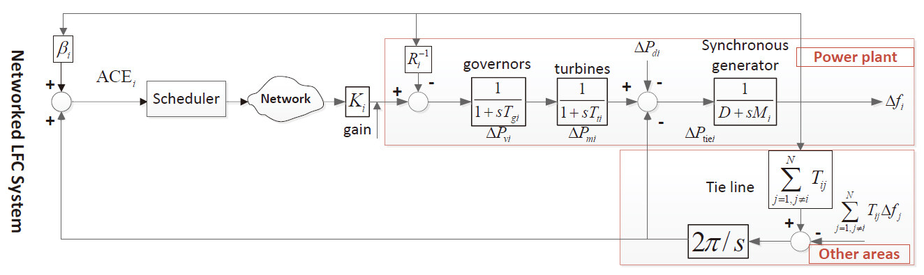
Figure 1. Multi-area decentralized power systems under scheduling protocols.

The system model is represented as[23, 25]:

$$ \begin{eqnarray} \begin{cases} \dot x(t)\, =Ax(t)-Bu(t)+D\omega(t), \cr y(t)\; \, =Cx(t), \end{cases} \end{eqnarray} $$

where $$ x(t)\in\mathbb{R}_{x} $$ is the state vector, $$ y(t)\in\mathbb{R}_{n_y} $$ is the measurement and $$ \omega(t)\in\mathbb{R}_{\omega} $$ is the disturbance, $$ u(t)\in\mathbb{R}_{u} $$ is the control input vector. The multi-area power systems consist of generators, turbines, and governors, where $$ \Delta P_{vi}, \Delta P_{mi}, \Delta P_{di} $$, and $$ \Delta f_i $$ denote the deviation of valve position, generator mechanical output, load, and the frequency of the $$ ith $$ sub-area, respectively. The area control error $$ ACE_i(s) $$ is

$$ \begin{eqnarray} ACE_i(s)=\beta_i \Delta f_i(s)+\Delta P_{tie-i}(s). \end{eqnarray} $$

The state and measured output signals are

$$ \begin{eqnarray*} &x_i^T(t)=[\Delta f_i(t), \Delta P_{tie-i}(t), \Delta P_{mi}, \Delta P_{vi}(t), \int ACE_i(t)] \\ &\omega_i(t)=\Delta P_{di}(t), \; y_i^T(t)=[ACE_i(t), \int ACE_i(t)] \end{eqnarray*} $$

where $$ x(t)=[x_1^T(t), \cdots, x_n^T(t)]^T $$, $$ \begin{align*} y(t) & = [y_1^T(t), \cdots, y_n^T(t)]^T\in \mathbb{R}_{n_y}, \\ \omega(t) & = [\omega_1^T(t), \cdots, \omega_n^T(t)]^T, \\ A & = [A_{ij}]_{n\times n}, \\ B & = \text{diag}\{B_1, \cdots, B_n\}, \\ C & = [C_1^T, \cdots, C_N^T]^T, \\ F & = \text{diag}\{F_1, \cdots, F_n\}, \\ C_i & = [\underbrace{0, \cdots, 0}_{i-1}, \bar{C}_i, \underbrace{0, \cdots, 0}_{N-i}] \end{align*} $$,

$$ \begin{eqnarray*} A_{ii}= \begin{bmatrix} -\frac{D_i}{M_i} & -\frac{1}{M_i} & \frac{1}{M_i} & 0 & 0 \\ 2 \pi \sum\limits_{j=1, j\neq i}^n T_{ij} & 0 & 0 & 0 & 0 \\ 0 & 0 & -\frac{1}{T_{chi}} & \frac{1}{T_{chi}} & 0 \\ -\frac{1}{R_i T_{gi}} & 0 & 0 & -\frac{1}{T_{gi}} & 0 \\ \beta_i & 1 & 0 & 0 & 0 \end{bmatrix}, \end{eqnarray*} $$

$$ \begin{eqnarray*} A_{ij}= \begin{bmatrix} 0 & 0 & 0 & 0 & 0 \\ -2 \pi T_{ij} & 0 & 0 & 0 & 0 \\ 0 & 0 & 0 & 0 & 0 \\ 0 & 0 & 0 & 0 & 0 \\ 0 & 0 & 0 & 0 & 0 \end{bmatrix}, F_i= \begin{bmatrix} -\frac{1}{M_i} \\ 0 \\ 0 \\ 0 \\ 0 \end{bmatrix}, B_i= \begin{bmatrix} 0 \\ 0 \\ 0 \\ \frac{1}{T_{gi}} \\ 0 \end{bmatrix}, \bar{C}_i^T= \begin{bmatrix} \beta_i & 0\\ 1 & 0 \\ 0 & 0 \\ 0 & 0 \\ 0 & 0 \end{bmatrix}. \end{eqnarray*} $$

The multi-area power system includes $$ N $$ controlled areas, $$ N $$ decentralized controllers, which are connected via the network. Then, measurement signals are given by $$ y_i(t)=C_i x(t)\in \mathbb{R}_{n_i}, i=1, \cdots, N, \sum\limits_{i=1}^N n_i=n_y $$. Based on the phasor measurement unit, sampling instants of $$ N $$ sensors are synchronized in different areas of power systems. Denote sampling instant by $$ s_q $$, satisfying that

$$ 0=s_0<s_1<\cdots<s_q<\cdots, s_{q+1}-s_q\leq \varrho, \lim\limits_{q\rightarrow +\infty} s_q= +\infty $$
, where $$ \varrho $$ is the maximum allowable transfer interval.

In this paper, we take imperfect network conditions into account, such as data loss and network-induced delay. Denote the sequence after packet loss by $$ \{s_k\}\subseteq\{s_q\} $$; that is, only at sampling instants $$ {s_k} $$, the input of the controller can be updated. For $$ i=1, \cdots, N $$, an uncertain, time-varying delay $$ v_{s_k}^i \in [0, \tau_M^i] $$ is assumed to occur, where $$ \tau_M^i $$ is delay upper bound of the $$ ith $$ channel and $$ \max\limits_{i=1, \cdots, N}\{\tau_M^i\}=\tau_M $$. Buffers are set to store and choose the largest communication delay $$ \tau_{s_k} $$ of power system channels, i.e., $$ \tau_{s_k}=\max\limits_{i=1, \cdots, N}\{v_{s_k}^i\} $$. Then, ZOH updating instant is $$ t_k=s_k+\tau_{s_k} $$. The transmission delay is assumed to be bound, satisfying:

$$ \begin{eqnarray} 0\leq\tau_{s_k}\leq\tau_M, \; t_{k+1}-t_k-\tau_{s_k}\leq \tau_M+\varrho=\bar{\tau}. \end{eqnarray} $$

Let $$ \hat{y}(s_k)=[\hat{y}_1^T (s_k) \cdots \hat{y}_N^T (s_k)]^T \in \mathbb{R}_{n_y} $$ denote the output signal transmitted to the scheduler. At instant $$ s_k $$, only one node can be active. Let $$ \iota_k\in \{1, \cdots, N\} $$ be the active output node at $$ s_k $$, which is dependent on the scheduling rule. Then, we have

$$ \begin{eqnarray} \hat{y}_i(s_k)= \begin{cases} y_i(s_k), i=\iota_k \\ \hat{y}_i(s_{k-1}), i\neq \iota_k \end{cases} \end{eqnarray} $$

Consider the scheduling error between output $$ y_i(s_k) $$ and the last available measurement $$ \hat{y}_i(s_{k-1}) $$:

$$ e_i(t)=-y_i(s_k)+\hat{y}_i(s_{k-1}), \; e(t)=col\{e_1(t), \cdots, e_N(t)\}, \; t\in[t_k, t_{k+1}), $$

where $$ \hat{y}_i(s_{-1})\triangleq 0, \; i=1, \cdots, N $$. In this paper, controllers and actuators in the $$ ith $$ area are event-driven. Let $$ L_i>0, i=1, \cdots, N $$ be node weighting matrices. Under TOD scheduling,

$$ \iota_k=\arg\max\limits_{i\in \{1, \cdots, N\}}|\sqrt{L_i}(-y_i(s_k)+\hat{y}_i(s_{k-1}))|^2. $$

Under RR scheduling protocol, the active node $$ \iota_k $$ is selected periodically:

$$\iota_k=\iota_{k+N}. $$

In the following, we will design the decentralized LFC law under the communication network. Similar to[23], a PI controller is used in this paper:

$$ \begin{eqnarray} u_i(t)=-K_{Pi} ACE_i(t)-K_{Ii}\int ACE_i(t). \end{eqnarray} $$

Therefore, dynamic model of the scheduled power systems under the decentralized LFC Equation (8) and imperfect network environments can be formalized as

$$ \begin{eqnarray} \begin{cases} \dot{x}(t)=Ax(t)-BK\hat{y}(s_k)+F\omega(t) \\ y(t)=Cx(t), t\in[t_k, t_{k+1}), \end{cases} \end{eqnarray} $$

where $$ u(t)=\sum\limits_{i=1}^N K_i y_i(t)=Ky(t), \; K=[K_1, \cdots, K_N] $$, $$ K_i=[K_{Pi}, K_{Ii}] $$.

2.2. Impulsive model and study objective

From Equation (5), one can obtain that

$$ \begin{eqnarray} e_i(t_{k+1})= \begin{cases} &C_i x(s_k)-C_i x(s_{k+1}), i=\iota_k \\ &C_i[x(s_k)-x(s_{k+1})]+e_i(t_k), i\neq \iota_k \end{cases} \end{eqnarray} $$

Define an artificial delay $$ \tau(t)=t-s_k $$, from which one arrives at

$$ \begin{eqnarray} 0\leq\tau_{s_k}\leq\tau(t)\leq s_{k+1}-s_k+\tau_{s_{k+1}}\leq\tau_M, \; \dot{\tau}(t)=1. \end{eqnarray} $$

From Equation (5) and Equation (9), the impulsive power system model can be

$$ \dot{x}(t)=Ax(t)-BKCx(t-\tau(t))-\sum\limits_{i=1, i\neq \iota_k}^N BK_i C_i e_i(t)+F\omega(t). $$

For system Equation (12), the initial condition of $$ x(t) $$ on $$ [-\tau_M, 0] $$ is supplemented as $$ x(t)=\phi(t), t\in[-\tau_M, 0] $$, with $$ \phi(0)=x_0 $$, where $$ \phi(t) $$ is a continuous function on $$ [-\tau_M, 0] $$.

Using scheduling scheme Equation (6) and Equation (7), this paper is to design the decentralized controller Equation (8) such that system Equation (12) is exponentially stable with a prescribed $$ H_\infty $$ performance $$ \gamma $$.

3. MAIN RESULTS

In the following, we first derive sufficient criteria under scheduling scheme Equation (6) and Equation (7) to ensure the exponential stability of system Equation (12) with a prescribed $$ H_\infty $$ performance. Then, criteria are proposed to design decentralized controllers under multi-channel transmission.

3.1. Stability analysis under the TOD scheduling scheme Equation (6)

Construct Lyapunov-Krasovskii functional candidate:

$$ \begin{eqnarray} \begin{aligned} V(t)=\sum\limits_{i=1}^N e_i^T(t)L_i e_i(t)+\Pi(t)+V_H, \end{aligned} \end{eqnarray} $$

where

$$ O>0, H_i>0, T>0, L_i>0, \alpha>0, S>0, i=1, \cdots, N, t\in[t_k, t_{k+1}) $$
,

$$ \begin{align*} V_H=&\sum\limits_{i=1}^N \int_{s_k}^t \tau_M e^{2\alpha(s-t)} \left\Vert \sqrt{H_i} C_i \dot x(s)\right\Vert^2 ds, \\ \Pi(t)=&\int_{t-\tau_M}^t e^{2\alpha(s-t)}x^T(s)Sx(s)ds+x^T(t)Ox(t)+\tau_M \int_{t-\tau_M}^t \int_s^t e^{2\alpha(s-t)}\dot{x}^T(v)T\dot{x}(v)dvds. \end{align*} $$

Remark 1$$ V_H $$is introduced to cope with reset conditions, which is continuous on $$ [t_k, t_{k+1}) $$, and does not grow in the jumps when $$ t=t_{k+1} $$ since

$$ -V_H(t_{k+1}^-)+V_H(t_{k+1})\leq-\sum\limits_{i=1}^N e^{-2\alpha\tau_M} \left\Vert\sqrt{H_i}C_i (-x(s_{k+1})+x(s_k))\right\Vert^2 $$

Theorem 1Under TOD scheduling scheme Equation (6), for given scalars $$ \tau_M, \alpha>0, \gamma>0 $$, impulsive system Equation (12) is exponentially stable with a prescribed $$ H_\infty $$ performance $$ \gamma $$, if there exist appropriate dimensions $$ Y $$ and real matrices $$ O>0, S>0, T>0, H_i>0, J_i>0, L_i>0, i=1, \cdots, N $$ such that

$$ \begin{eqnarray} \begin{bmatrix} \Xi_{11} & \ast & \ast \\ \Xi_{21} & \Xi_{22} & \ast \\ \Xi_{31} & 0 & \Xi_{33} \end{bmatrix}<0, \end{eqnarray} $$

$$ \begin{eqnarray} \begin{bmatrix} T & Y^T \\ Y & T \end{bmatrix}>0, \end{eqnarray} $$

$$ \begin{eqnarray} \Omega_i= \begin{bmatrix} \Omega_{11} & \Omega_{12} \\ \ast & \Omega_{22} \end{bmatrix}<0 \end{eqnarray} $$

are feasible for $$ i, j=1, \cdots, N $$, where

$$ \begin{eqnarray*} &\Xi_{11}= \begin{bmatrix} \Psi_{11} & \Psi_{12} & \Psi_{13} & \Psi_{14} & \Psi_{15} \\ \ast & \Psi_{22} & \Psi_{23} & 0 & 0 \\ \ast & \ast & \Psi_{33} & 0 & 0 \\ \ast & \ast & \ast & \Psi_{44} & 0 \\ \ast & \ast & \ast & \ast & \Psi_{55} \end{bmatrix}, \bar{\xi}_i= \begin{cases} [-PBK_2C_2, \cdots, -PBK_NC_N], \iota_k=1 \\ [-PBK_1C_1, \cdots, -PBK_{N-1}C_{N-1}], \iota_k=N \\ [-PBK_1C_1, \cdots, -PBK_jC_{j|j\neq \iota_k}, \cdots, -PBK_NC_N], \iota_k\neq1, N \end{cases} \\ &\phi_i= \begin{cases} diag\{\psi_2, \cdots, \psi_N\}, \iota_k=1 \\ diag\{\psi_1, \cdots, \psi_{N-1}\}, \iota_k=N \\ diag\{\psi_1, \cdots, \psi_{j|j\neq \iota_k}, \cdots, \psi_N\}, \iota_k\neq1, N \end{cases}, \pi_i= \begin{cases} [BK_2C_2, \cdots, BK_NC_N], \iota_k=1 \\ [BK_1C_1, \cdots, BK_{N-1}C_{N-1}], \iota_k=N \\ [BK_1C_1, \cdots, BK_jC_{j|j\neq \iota_k}, \cdots, BK_NC_N], \iota_k\neq1, N. \end{cases}\\ &\Psi_{11}=OA+A^TO+2\alpha O+S+T, \Psi_{13}=-Y^T, \Psi_{14}=\chi_i, \Psi_{23}=Y^T-T, F_i=[A, BKC, 0, \pi_i, F], \\ &\Psi_{22}=2T-Y-Y^T, \Psi_{33}=T-S, \Psi_{44}=\chi_i, \Omega_{11}=-\frac{1-2\alpha\tau_M}{N-1}L_i+J_i, \Psi_{12}=-OBKC-T+Y^T, \\ &\chi_i=[-OBK_1C_1, \cdots, -OBK_NC_N], \Omega_{22}=L_i-H_i e^{-2\alpha\tau_M}, \Xi_{22}=diag\{-T, -H_1, \cdots, -H_N\}, \\ &\Psi_{15}=OF, \Omega_{12}=L_i, \Xi_{21}=[\tau_M TF_i, \sqrt{\tau_M}H_1C_1F_1, \cdots, \sqrt{\tau_M}H_NC_NF_N], \Psi_{55}=-\gamma^2I, \\ &\psi_j=-\frac{1}{\tau_M}J_j+2\alpha L_j, \Theta=\tau_M^2 T+\tau_M\sum\limits_{i=1}^N C_i^T H_iC_i, \Xi_{31}=[C, 0, \cdots, 0]. \end{eqnarray*} $$

Proof: Differentiating $$ V(t) $$ along Equation (12) and applying Wirtinger-based integral inequality[26], we can obtain

$$ \begin{eqnarray} \begin{aligned} &\dot{V}(t)+2\alpha V(t)-\frac{1}{\tau_M}\sum\limits_{i=1, i\neq \iota_k}^N |\sqrt{J_i}C_i e_i(t)|^2-2\alpha|\sqrt{L_{\iota_k}}e_{\iota_k}(t)|^2+|y(t)|^2-\gamma^2 |\omega(t)|^2\leq-\frac{1}{\tau_M}\sum\limits_{l=1, l\neq i}^N |\sqrt{J_l}C_le_l(t)|^2 \\ &-\gamma^2|\omega(t)|^2-e^{-2\alpha \tau_M}x^T(t-\tau_M)Sx(t-\tau_M)+|y(t)|^2+\dot{x}^T(t)\Theta \dot{x}(t)-e^{-2\alpha\tau_M}\tau_M\int_{t-\tau_M}^t \dot{x}^T(s)T\dot{x}(s)ds\\ &+2\alpha\sum\limits_{l=1, l\neq i}^N e_l^T(t)C_lL_lC_le_l(t)+2x^T(t)O\dot{x}(t)+x^T(t)(2\alpha O+S)x(t), \end{aligned} \end{eqnarray} $$

where $$ \xi_i(t)=col\{x(t), x(t-\tau(t)), x(t-\tau_M), \bar{\xi}_i(t), \omega(t)\} $$.

We use the reciprocally convex approach[27] to deal with the cross item in Equation (18). By using Schur's complement, one can get

$$ \begin{eqnarray} \begin{aligned} \dot{V}(t)+2\alpha V(t)-\frac{1}{\tau_M}\sum\limits_{i=1, i\neq \iota_k}^N |\sqrt{J_i}C_i e_i(t)|^2-2\alpha|\sqrt{L_{\iota_k}}e_{\iota_k}(t)|^2+|y(t)|^2-\gamma^2 |\omega(t)|^2<0. \end{aligned} \end{eqnarray} $$

In the following, we will prove that

(ⅰ) with $$ \omega(t)=0 $$, the impulsive system Equation (12) is exponentially stable.

Since $$ \frac{d}{dt}e^{2\alpha t}V(t)=e^{2\alpha t}(\dot{V}(t)+2\alpha V(t)) $$ and $$ V(t) $$ is continuous in $$ t\in[t_k, t_{k+1}) $$, the integration of Equation (19) yields

$$ \begin{eqnarray} \begin{aligned} e^{2\alpha t}V(t)-e^{2\alpha t_k}V(t_k)\leq \int_{t_k}^t e^{2\alpha s}ds[2\alpha|\sqrt{L_{\iota_k}}e_{\iota_k}(t)|^2+\frac{1}{\tau_M}\sum\limits_{i=1, i\neq \iota_k}^{N}|\sqrt{J_i}C_i e_i(t)|^2]. \end{aligned} \end{eqnarray} $$

It follows from $$ \int_{t_k}^t e^{2\alpha(s-t)}ds\leq \tau_M $$ that

$$ \begin{eqnarray} V(t_{k+1})\leq \Theta_k+e^{2\alpha(t_k-t_{k+1})}V(t_k), \end{eqnarray} $$

where

$$ \begin{eqnarray} \begin{aligned} \Theta_k=\sum\limits_{j=1}^N [-V_H(t_{k+1}^-)+|\sqrt{L_{\iota_k}}e_{\iota_k}(t_{k+1})|^2-|\sqrt{L_{\iota_k}}e_{\iota_k}(t_k)|^2+V_H(t_{k+1})]+\sum\limits_{i=1, i\neq \iota_k}^N |\sqrt{J_i} C_i e_i(t)|^2+2\alpha\tau_M|\sqrt{L_{\iota_k}}e_{\iota_k}(t_k)|^2. \end{aligned} \end{eqnarray} $$

Then taking Equation (17) and Equation (22) into account, denoting $$ \kappa_i=[e_i(t_k), C_i[-x(s_{k+1})+x(s_k)]]^T $$, we have

$$ \begin{eqnarray} \begin{aligned} \Theta_k\leq-|(\sqrt{H_{\iota_k}}e^{-2\alpha\tau_M}-\sqrt{L_{\iota_k}})C_{\iota_k}[x(s_k)-x(s_{k+1})]|^2+\sum\limits_{i=1, i\neq \iota_k}^N \kappa_i\Omega_i\kappa_i\leq0. \end{aligned} \end{eqnarray} $$

Hence, one can conclude that

$$ \begin{eqnarray} \begin{aligned} V(t)\leq \sum\limits_{i=1, i\neq \iota_k}^N |\sqrt{J_i}e_i(t_k)|^2+e^{2\alpha(t_0-t)}V(t_0)+2\alpha\tau_M |\sqrt{L_{\iota_k}}e_{\iota_k}(t_k)|^2. \end{aligned} \end{eqnarray} $$

From Equation (24), we have

$$ \begin{eqnarray*} V(t)\geq \lambda_{min}\{O\}|x(t)|^2+\sum\limits_{i=1}^N|\sqrt{L_i}e_i(t)|^2, \end{eqnarray*} $$

which implies that

$$ \begin{eqnarray*} \lambda_{min}\{O\}|x(t)|^2\leq (2\alpha\tau_M-1)|\sqrt{L_{\iota_k}}e_{\iota_k}(t)|^2+\sum\limits_{i=1, i\neq \iota_k}^N |\sqrt{J_i-L_i}e_i(t)|^2+e^{2\alpha(t_0-t)}V(t_0). \end{eqnarray*} $$

It follows from $$ \Omega_i<0 $$ that for $$ t\geq t_0 $$

$$ \begin{eqnarray} \lambda_{min}\{O\}|x(t)|^2\leq e^{2\alpha(t_0-t)}V(t_0). \end{eqnarray} $$

For $$ t<t_0 $$, the system takes the form $$ \dot{x}=Ax(t)+F\omega(t) $$, then its corresponding solution is given by

$$ \begin{eqnarray} x(t)=e^{At}x(0)+\int_0^t e^{A(-s+t)}F\omega(s)ds. \end{eqnarray} $$

Clearly, there exists the maximum of $$ |x(t)| $$ for $$ t\in[t_0-\tau_M, t_0] $$. Thus, $$ V(t_0)\leq \mu \|x_{t_0}\|_W^2+\sum\limits_{i=1}^N e_i^T(t_0)L_ie_i(t_0) $$ for some $$ \mu>0 $$.

Therefore, the exponential stability of the system Equation (12) with $$ \omega(t)=0 $$ is guaranteed.

Next, we will show that

(ⅱ) under the zero initial condition, the inequality $$ \|y\|_{L_2}\leq\gamma\|\omega\|_{L_2} $$ holds for any nonzero $$ \omega\in L_2[0, +\infty) $$.

From Equation (19), we obtain that for $$ t\in[t_k, t_{k+1}) $$,

$$ \begin{eqnarray} \begin{aligned} |y(t)|^2-\gamma^2|\omega(t)|^2\leq -\dot{V}(t)+2\alpha|\sqrt{L_{\iota_k}}e_{\iota_k}(t)|^2+\frac{1}{\tau_M}\sum\limits_{i=1, i\neq \iota_k}^N |\sqrt{J_i}C_ie_i(t)|^2. \end{aligned} \end{eqnarray} $$

Integrating Equation (27) on $$ t $$ from $$ t_k $$ to $$ t_{k+1}^- $$ yields

$$ \begin{eqnarray} \begin{aligned} \int_{t_k}^{t_{k+1}^-}|y(s)|^2-\gamma^2|\omega(s)|^2ds+V(t_{k+1})\leq V(t_k)+\Theta_k\leq V(t_k). \end{aligned} \end{eqnarray} $$

Then, by summing Equation (28) on $$ k $$ from $$ 0 $$ to $$ \rho $$, where $$ \rho\rightarrow +\infty $$, we have

$$ \begin{eqnarray} \int_{t_0}^{t_{\rho+1}^-}(|y(s)|^2-\gamma^2|\omega(s)|^2)ds\leq V(t_0). \end{eqnarray} $$

Under the zero initial condition, $$ \int_0^{+\infty} y^T(s)y(s)ds\leq \int_0^{+\infty}\gamma^2\omega^T(s)\omega(s)ds $$. Therefore, one can derive that under the zero initial condition, $$ \|y\|_{L_2}\leq\gamma\|\omega\|_{L_2} $$ for any nonzero $$ \omega\in L_2[0, +\infty) $$. This completes the proof.

Remark 2The feasibility of the linear martix inequalities has been sufficiently explained in[23, 28]. Due to page limitations, this part is omitted here.

3.2. Stability analysis under the RR scheduling scheme Equation (7)

Construct the following Lyapunov-Krasovskii functional candidate:

$$ \begin{eqnarray} \begin{aligned} V(t)=\Pi(t)+V_H+V_L, \; k\geq N-1, \; t\in[t_k, t_{k+1}), \end{aligned} \end{eqnarray} $$

where

$$ \begin{align*} &V_H= \begin{cases} \sum\limits_{i=1}^{N-1}\tau_M\int_{s_k}^t e^{2\alpha(s-t)}|\sqrt{H_i} C_i\dot{x}(s)ds, \; k\neq N-1, \\ \sum\limits_{i=1}^{N-1}\tau_M\int_{s_0}^t e^{2\alpha(s-t)}|\sqrt{H_i} C_i\dot{x}(s)ds, \; k=N-1, \\ \end{cases} \\ &H_i=(N-1)L_i e^{2\alpha(N-1)\tau_M}, V_L=\sum\limits_{i=1}^{N-1}\frac{t_{k+1}-t}{i\tau_M}|\sqrt{L_{\iota_{k-j}}}e_{\iota_{k-j}}(t)|^2. \end{align*} $$

Similar to Theorem 5.2 in[29], we establish the following result.

Theorem 2Under RR scheduling scheme Equation (7), given $$ \tau_M>0 $$ and $$ \alpha>0 $$, assume that there exist matrices $$ O>0, S>0, T>0, L_i>0, i=1, \cdots, N $$ and $$ Y $$ with appropriate dimensions such that Equation (15) and Equation (16) are feasible with $$ J_i=\frac{L_i}{N-1} $$, where $$ G_i $$ is given by Equation (30). Then, system Equation (12) is exponentially stable with a prescribed $$ H_\infty $$ performance $$ \gamma $$.

Proof: The detailed derivation process can refer to[29] and the proof of Theorem 1, which is omitted here due to the limited pages.

3.3. Controller Design under the TOD scheduling scheme Equation (6)

Theorem 3.3.Under TOD scheduling scheme Equation (6), for given matrices $$ A, B, C, F $$, and scalars $$ \tau_M, \alpha>0, \gamma>0, \zeta>0 $$, system Equation (12) is exponentially stable with a prescribed $$ H_\infty $$ performance $$ \gamma $$, if there exist real matrices

$$ Z>0, \tilde{S}>0, \tilde{T}>0, i, j=1, \cdots, N, \tilde{J}_i>0, H_i>0, \tilde{L}_i>0 $$
and appropriate dimensions $$ \tilde{Y}, \beth, \digamma $$ such that

$$ \begin{align} \begin{split} & min \ tr\left\{\sum\limits_{i=1}^N H_i h_i\right\}\\ & s.t. \ Equation (17), Equation (32)^*, Equation (33), Equation (34), Equation (35) \end{split} \end{align} $$

$$ \begin{eqnarray} \begin{bmatrix} \tilde{\Xi}_{11} & \ast & \ast \\ \tilde{\Xi}_{21} & \tilde{\Xi}_{22} & \ast \\ \tilde{\Xi}_{31} & 0 & \tilde{\Xi}_{33} \end{bmatrix}<0, \end{eqnarray} $$

$$ \begin{eqnarray} \begin{bmatrix} \tilde{T} & \tilde{Y}^T \\ \tilde{Y} & \tilde{T} \end{bmatrix}>0, \end{eqnarray} $$

$$ \begin{eqnarray} \begin{bmatrix} h_i & \ast \\ I & H_i \end{bmatrix}>0, \end{eqnarray} $$

$$ \begin{eqnarray} \begin{bmatrix} -\zeta I & (\beth C-CZ)^T \\ \beth C-CZ & -I \end{bmatrix}<0, \end{eqnarray} $$

is solvable, and the controller gain is given by $$ K=\digamma\beth^{-1} $$, where $$ Equation (32)^* $$ is equivalent to Equation (32) by replacing $$ -H_i^{-1} -Z^T\tilde{T}_r^{-1} Z $$ with $$ -h_i, \rho^2 \tilde{T}_r-2\rho Z $$, and

$$ \begin{eqnarray*} &\tilde{\Xi}_{11}= \begin{bmatrix} \tilde{\Psi}_{11} & \tilde{\Psi}_{12} & \tilde{\Psi}_{13} & \tilde{\Psi}_{14} & \tilde{\Psi}_{15} \\ \ast & \tilde{\Psi}_{22} & \tilde{\Psi}_{23} & 0 & 0 \\ \ast & \ast & \tilde{\Psi}_{33} & 0 & 0 \\ \ast & \ast & \ast & \tilde{\Psi}_{44} & 0 \\ \ast & \ast & \ast & \ast & \tilde{\Psi}_{55} \end{bmatrix}, \\ &\tilde{\phi}_i= \begin{cases} diag\{\tilde{\psi}_2, \cdots, \tilde{\psi}_N\}, \iota_k=1 \\ diag\{\tilde{\psi}_1, \cdots, \tilde{\psi}_{N-1}\}, \iota_k=N \\ diag\{\tilde{\psi}_1, \cdots, \tilde{\psi}_{j|j\neq \iota_k}, \cdots, \tilde{\psi}_N\}, \iota_k\neq1, N \end{cases}\\ &\tilde{\bar{\xi}}_i= \begin{cases} [-BK_2C_2Z, \cdots, -BK_NC_NZ], \iota_k=1 \\ [-BK_1C_1Z, \cdots, -BK_{N-1}C_{N-1}Z], \iota_k=N \\ [-BK_1C_1Z, \cdots, -BK_jC_{j|j\neq \iota_k}Z, \cdots, -BK_NC_NZ], \iota_k\neq1, N \end{cases}\\ &\tilde{\psi}_j=-\frac{1}{\tau_M}\tilde{J}_j+2\alpha \tilde{L}_j, \tilde{\Xi}_{33}=-I, \tilde{\Psi}_{11}=AZ+ZA^T+2\alpha Z+\tilde{S}+\tilde{T}, \tilde{\Psi}_{12}=-BKCZ-\tilde{T}+\tilde{Y}^T, \tilde{\Psi}_{22}=2\tilde{T}-\tilde{Y}-\tilde{Y}^T, \tilde{T}=ZTZ, \\ &\tilde{\Psi}_{23}=\tilde{Y}^T-\tilde{T}, \tilde{\chi}_i=[-BK_1C_1Z, \cdots, -BK_NC_NZ], \tilde{\Psi}_{33}=\tilde{T}-\tilde{S}, \tilde{\Psi}_{14}=\tilde{\chi}_i, \tilde{\Psi}_{44}=\tilde{\phi}_i, \tilde{\Psi}_{55}=-\gamma^2I, \tilde{\Psi}_{13}=-\tilde{Y}^T, \tilde{S}=ZSZ, \\ &\tilde{\Xi}_{31}=[CZ, 0, \cdots, 0], \tilde{\Xi}_{22}=diag\{-Z\tilde{T}^{-1}Z, -H_1^{-1}, \cdots, -H_N^{-1}\}, \tilde{\Xi}_{21}^T=[\tau_M F_i, \sqrt{\tau_M}C_1F_1, \cdots, \sqrt{\tau_M}C_NF_N], \tilde{Y}=ZYZ. \end{eqnarray*} $$

Proof: Let $$ Z=O^{-1}, \tilde{J}_i=ZJ_iZ, \tilde{L_i}=ZL_iZ, i=1, \cdots, N $$. Pre- and post-multiplying Equation (15) and Equation (16) with

$$ \begin{align*} diag\{Z, \cdots, Z, I, T^{-1}, H_1^{-1}, \cdots, H_N^{-1}, I, Z\} \end{align*} $$

and their transposes, respectively. For the nonlinear terms $$ -Z\tilde{T}_r^{-1}Z, r=1, 2 $$ and $$ -H_i^{-1} $$, using inequalities $$ -Z\tilde{T}_r^{-1}Z\leq\rho^2 \tilde{T}_r-2\rho Z $$ and the cone complementary linearization algorithm in[27], one can obtain $$ Equation (32)^* $$. By solving the minimization problem Equation (31), system Equation (12) is exponentially stable with a prescribed $$ H_\infty $$ performance $$ \gamma $$ and $$ K=\digamma\beth^{-1} $$.

3.4. Controller design under the RR scheduling scheme Equation (7)

Similar to Theorem 5.2 in[29], we establish Theorem 4.

Theorem 4Under the RR scheduling scheme Equation (7), for given matrices $$ A, B, C, F $$, and scalars $$ \tau_M, \alpha>0, \gamma>0, \zeta>0 $$, system Equation (12) is exponentially stable with a prescribed $$ H_\infty $$ performance $$ \gamma $$, if there exist real matrices $$ Z>0, \tilde{S}>0, \tilde{T}>0, \tilde{L}_i>0, i=1, \cdots, N $$ and $$ \tilde{Y}, \beth, \digamma $$ with appropriate dimensions such that Equation (31) is solvable with $$ J_i=\frac{L_i}{N-1} $$, where $$ H_i $$ is given by Equation (30). The controller gain is given by $$ K=\digamma\beth^{-1} $$.

Proof: The detailed derivation process can refer to[29] and the proof of Theorem 3, which is omitted here.

4. AN ILLUSTRATIVE EXAMPLE

In the following, we use a three-area power system[23, 24, 28] interconnected by the shared communication network to demonstrate the effectiveness of main results. Parameters are listed in Table 1.

Table 1

Configuration of three-area power systems

$$ Parameter $$$$ T_{ch}(s) $$$$ T_g(s) $$$$ R $$$$ D $$$$ \beta $$$$ M(s) $$
$$ Area 1 $$0.300.370.051.0$$ \frac{1}{R_1}+D_1 $$10
$$ Area 2 $$0.170.400.051.5$$ \frac{4}{R_2}+D_2 $$10
$$ Area 3 $$0.200.350.051.8$$ \frac{3}{R_3}+D_3 $$12
$$ T_{12}=0.20, T_{13}=0.12, T_{23}=0.25(pu/rad) $$

Case 1: Stability of the studied system under TOD scheduling scheme Equation (6) and $$ \omega(t)=0 $$.

Assume parameters are chosen as $$ \tau_M=0.1s, \gamma=10, \rho=0.63 $$. We apply Theorem 3 which yields $$ K_1=[0.2393, 0.0224] $$, $$ K_2=[0.2379, -0.1352] $$, $$ K_3=[0.2324, 0.1965] $$.

Correspondingly, state responses and the switching behavior of active nodes are illustrated by Figure 2 and 3, respectively. Clearly, the designed dynamics output feedback controllers can stabilize the three-area power system under the TOD scheduling scheme Equation (6) in the absence of disturbance.

Networked scheduling for decentralized load frequency control

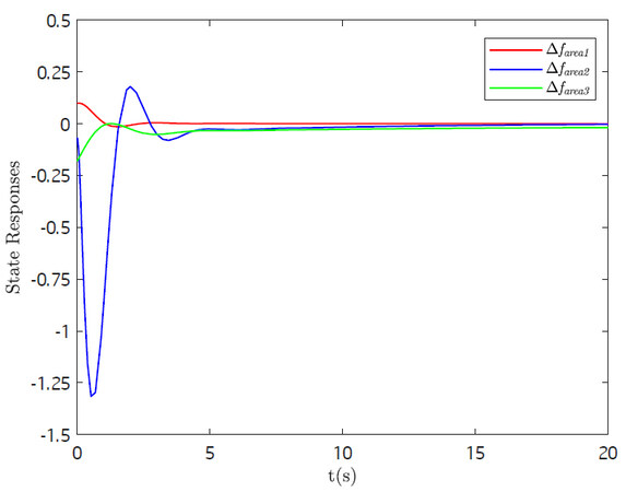
Figure 2. State responses of case 1.

Networked scheduling for decentralized load frequency control

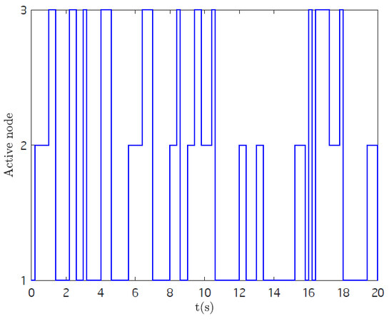
Figure 3. The switching behavior of active nodes of case 1.

Case 2: Stability of the studied system under RR scheduling scheme Equation (7) and $$ \omega(t)=0 $$.

To compare with the TOD protocol Equation (6), we use the same parameters as case 1. We apply Theorem 4 which yields $$ K_1=[0.1876, 0.0184] $$, $$ K_2=[0.1899, -0.1596] $$, $$ K_3=[0.1824, 0.1498] $$. Then, state responses and the switching behavior of active nodes are depicted in Figure 4 and 5. From Figure 2-5, one can obtain that the system can be stable under both scheduling protocols Equation (6), Equation (7). Compared with RR protocol, TOD protocol can achieve dynamic scheduling, which makes the control process more efficient.

Networked scheduling for decentralized load frequency control

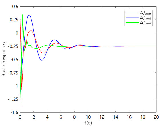
Figure 4. State responses of case 2.

Networked scheduling for decentralized load frequency control

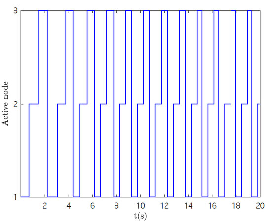
Figure 5. The switching behavior of active nodes of case 2.

Case 3: Stability of the studied system under TOD scheduling scheme Equation (6) and $$ \omega(t)\neq 0 $$.

According to Theorem 1-4, TOD protocol can degrade into RR protocol under certain conditions. In this case, we take the TOD protocol Equation (6) as an example to verify the anti-disturbance performance of the studied system. Under the disturbance $$ \omega(t) $$ shown in Figure 6, we obtain controller gains $$ K_1=[0.4005, -0.1702] $$, $$ K_2=[0.4839, -0.2094] $$, $$ K_3=[0.4914, -0.4009] $$. State responses of the system are depicted in Figure 7. The designed decentralized controllers under the TOD protocol Equation (6) can ensure system stability with load disturbances.

Networked scheduling for decentralized load frequency control

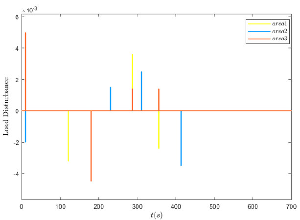
Figure 6. Disturbance of case 3.

Networked scheduling for decentralized load frequency control

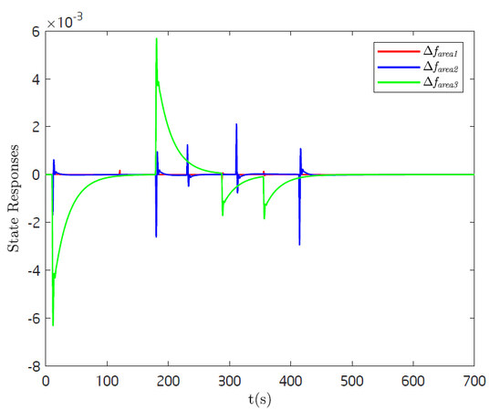
Figure 7. State responses of case 3.

5. CONCLUSIONS

This paper has designed $$ H_\infty $$ output feedback decentralized load frequency controllers for multi-area power systems under the shared but band-limited network. TOD and RR protocols have been used to improve communication efficiency. Since transmission priority has been well designed under scheduling protocols, a higher control performance has been obtained. Then, decentralized output feedback controllers with the prescribed performance have been designed in different areas. Finally, an example has verified the effectiveness of main results.

DECLARATIONS

Authors' contributions

Made substantial contributions to the research, idea generation, algorithm design, performed critical review, commentary and revision, as well as provided administrative, technical, and material support: Peng C

Conceived and designed the experiments, analyzed simulation results, wrote and edited the original draft: Yang H

Financial support and sponsorship

This work was supported in part by the National Natural Science Foundation of China under Grant 62173218, and the International Corporation Project of Shanghai Science and Technology Commission under Grant 21190780300.

Availability of data and materials

Not applicable.

Conflicts of interest

All authors declared that there are no conflicts of interest.

Ethical approval and consent to participate

Not applicable.

Consent for publication

Not applicable.

Copyright

© The Author(s) 2022.

REFERENCES

1. Mohandes B, El Moursi MS, Hatziargyriou N, El Khatib S. A review of power system flexibility with high penetration of renewables. IEEE Trans Power Syst 2019;34:3140-55.

2. Ranjan M, Shankar R. A literature survey on load frequency control considering renewable energy integration in power system: Recent trends and future prospects. J Energy Stor 2022;45:103717.

3. Peng C, Li F. A survey on recent advances in event-triggered communication and control. Inform Sci 2018;457:113-25.

4. Zhou Q, Shahidehpour M, Paaso A, et al. Distributed control and communication strategies in networked microgrids. IEEE Communic Surv & Tutori 2020;22:2586-633.

5. Shang Y. Group consensus of multi-agent systems in directed networks with noises and time delays. Int J Syst Sci 2015;46:2481-92.

6. Alhelou HH, Hamedani-Golshan ME, Zamani R, Heydarian-Forushani E, Siano P. Challenges and opportunities of load frequency control in conventional, modern and future smart power systems: a comprehensive review. Energies 2018;11:2497.

7. Yan Z, Xu Y. Data-driven load frequency control for stochastic power systems: a deep reinforcement learning method with continuous action search. IEEE Trans Power Syst 2018;34:1653-56.

8. Peng C, Wu J, Tian E. Stochastic event-triggered $H_\infty$ control for networked systems under denial of service attacks. IEEE Trans Syst, Man, Cybern: Systems 2021; doi: 10.1109/TSMC.2021.3090024.

9. Shangguan XC, He Y, Zhang CK, et al. Control performance standards-oriented event-triggered load frequency control for power systems under limited communication bandwidth. IEEE Trans Contr Syst Technol 2021;30:860-68.

10. Tian E, Peng C. Memory-based event-triggering $H_\infty$ load frequency control for power systems under deception attacks. IEEE Trans Cybern 2020;50:4610-18.

11. Peng C, Sun H, Yang M, Wang YL. A survey on security communication and control for smart grids under malicious cyber attacks. IEEE Trans Syst, Man, Cybern: Systems 2019;49:1554-69.

12. Wang D, Chen F, Meng B, Hu X, Wang J. Event-based secure $H_\infty$ load frequency control for delayed power systems subject to deception attacks. Appl Mathem Comput 2021;394:125788.

13. Wu J, Peng C, Yang H, Wang YL. Recent advances in event-triggered security control of networked systems: a survey. Int J Syst Sci 2022;0:1-20.

14. Freirich D, Fridman E. Decentralized networked control of systems with local networks: a time-delay approach. Automatica 2016;69:201-9.

15. Liu K, Fridman E, Hetel L, Richard JP. Sampled-data stabilization via round-robin scheduling: a direct Lyapunov-Krasovskii approach. IFAC Proceed Vol 2011;44:1459-64.

16. Ding D, Wang Z, Han QL, Wei G. Neural-network-based output-feedback control under round-robin scheduling protocols. IEEE trans cybern 2018;49:2372-84.

17. Zou L, Wang Z, Han QL, Zhou D. Full information estimation for time-varying systems subject to Round-Robin scheduling: A recursive filter approach. IEEE Trans Syst, Man, Cybern: Systems 2019;51:1904-16.

18. Zhang XM, Han QL, Ge X, et al. Networked control systems: a survey of trends and techniques. IEEE/CAA J Autom Sinica 2019;7:1-17.

19. Liu K, Fridman E, Hetel L. Network-based control via a novel analysis of hybrid systems with time-varying delays. In: 2012 IEEE 51st IEEE Confer Decis Contr (CDC). IEEE; 2012. pp. 3886-91.

20. Zhang J, Peng C, Xie X, Yue D. Output feedback stabilization of networked control systems under a stochastic scheduling protocol. IEEE trans cybern 2019;50:2851-60.

21. Liu K, Fridman E, Johansson KH. Networked control with stochastic scheduling. IEEE Trans Autom Contr 2015;60:3071-76.

22. Zhang J, Peng C. Networked $H_\infty$ filtering under a weighted TOD protocol. Automatica 2019;107:333-41.

23. Peng C, Zhang J, Yan H. Adaptive event-triggering $H_\infty$ load frequency control for network-based power systems. IEEE Trans Industr Electr 2017;65:1685-94.

24. Sun H, Peng C, Yue D, Wang YL, Zhang T. Resilient load frequency control of cyber-physical power systems under QoS-dependent event-triggered communication. IEEE Trans Syst, Man, Cybernet: Systems 2020;51:2113-22.

25. Shang Y. Median-based resilient consensus over time-varying random networks. IEEE Trans Circ Syst Ⅱ: Express Briefs 2021;69:1203-7.

26. Seuret A, Gouaisbaut F. Wirtinger-based integral inequality: application to time-delay systems. Automatica 2013;49:2860-66.

27. El Ghaoui L, Oustry F, AitRami M. A cone complementarity linearization algorithm for static output-feedback and related problems. IEEE trans autom contr 1997;42:1171-76.

28. Peng C, Li J, Fei M. Resilient Event-Triggering $H_\infty$ load frequency control for multi-area power systems with energy-limited DoS attacks. IEEE Trans Power Syst 2016;32:4110-18.

29. Liu K, Fridman E, Xia Y. Networked control under communication constraints. Springer; 2020.

Cite This Article

Export citation file: BibTeX | RIS

OAE Style

Peng C, Yang H. Networked scheduling for decentralized load frequency control. Intell Robot 2022;2(3):298-312. http://dx.doi.org/10.20517/ir.2022.27

AMA Style

Peng C, Yang H. Networked scheduling for decentralized load frequency control. Intelligence & Robotics. 2022; 2(3): 298-312. http://dx.doi.org/10.20517/ir.2022.27

Chicago/Turabian Style

Peng, Chen, Hongchenyu Yang. 2022. "Networked scheduling for decentralized load frequency control" Intelligence & Robotics. 2, no.3: 298-312. http://dx.doi.org/10.20517/ir.2022.27

ACS Style

Peng, C.; Yang H. Networked scheduling for decentralized load frequency control. Intell. Robot. 2022, 2, 298-312. http://dx.doi.org/10.20517/ir.2022.27

About This Article

© The Author(s) 2022. Open Access This article is licensed under a Creative Commons Attribution 4.0 International License (https://creativecommons.org/licenses/by/4.0/), which permits unrestricted use, sharing, adaptation, distribution and reproduction in any medium or format, for any purpose, even commercially, as long as you give appropriate credit to the original author(s) and the source, provide a link to the Creative Commons license, and indicate if changes were made.

Data & Comments

Data

Views
1224
Downloads
637
Citations
0
Comments
0
1

Comments

Comments must be written in English. Spam, offensive content, impersonation, and private information will not be permitted. If any comment is reported and identified as inappropriate content by OAE staff, the comment will be removed without notice. If you have any queries or need any help, please contact us at support@oaepublish.com.

0
Author's Talk
Download PDF
Cite This Article 11 clicks
Like This Article 1 likes
Share This Article
Scan the QR code for reading!
See Updates
Contents
Figures
Related
Intelligence & Robotics
ISSN 2770-3541 (Online)
Follow Us

Portico

All published articles are preserved here permanently:

https://www.portico.org/publishers/oae/

Portico

All published articles are preserved here permanently:

https://www.portico.org/publishers/oae/