

Evaluating the interpretability of a hierarchical fuzzy rule-based model for shipbreaking
 0
0 
Abstract
Machine learning models can provide valuable decision support in many real-world applications. However, a model must be interpretable to those using it. This paper explores the use of post-hoc model interpretability methods in combination with an intrinsically interpretable model design to create a model that is interpretable to both a model designer and a model end user. A hierarchical fuzzy rule-based model is trained with a genetic algorithm on a real-world shipbreaking use case and the performance-interpretability trade-off of the model with respect to a random forest model is discussed. Further, an interesting pattern was found using the post-hoc interpretability method SHapley Additive exPlanations (SHAP), with potential implications for the future design of hierarchical fuzzy rule-based models.
Keywords
1. INTRODUCTION
1.1. Importance of interpretability in machine learning
Machine learning models can identify patterns in large amounts of data that humans would not be able to detect. These patterns can aid in making better, more informed decisions. However, blindly trusting these models can lead to unfairness or wrong decisions. Therefore, the importance of interpretability for machine learning models used as decision support tools is widely recognized. Humans who work with decision support tools must be able to understand why a model gives certain predictions, so that they may decide whether to trust the model's output. Furthermore, the European Union's Artificial Intelligence (AI) Act outlines the interpretability requirements of a model based on its risk level[1].
Interpretability in a decision support model is defined here as the ability of a human user of the model to understand the model output and how it was created, using the model itself and the input data as context. There are many ways to categorize the interpretability of a model. Here a framework of when the interpretability is incorporated in the model can be used. The two primary temporal categories discussed in this work are understanding the model itself (intrinsic interpretability), and interpreting the model after it has been created (post-hoc interpretability). For a model itself to be interpretable, it must be simple or constrained in such a way that a human may understand it[2]. With a method such as feature importance, an attempt is made to understand a model after it has been created, because it is too complex for a human to understand as it is. This is often referred to as interpreting a "black box" model. A further important aspect of interpretability, as it is defined here, is who seeks to benefit from the model interpretability. Here, several "audiences" can be defined: the model designers, the model end users and those about whom the model makes decisions. In this application, the focus is on the model designers and the model end users, as for this use case, the model end users will provide explanations to those about whom the model makes decisions. The model end users for this application of shipbreaking are the ship inspectors.
1.2. Interpretable fuzzy rule-based models
Fuzzy rule-based models (FRBMs) lend themselves naturally to being interpretable. Fuzzy sets allow for an encoding of real-world data that better reflects the uncertainty and "fuzziness" of those data[3]. The linguistic "if-then" rules are formatted in the same manner that humans reason, and can be written by data set experts for smaller input applications. Though these aspects of FRBMs can lead to interpretability, there are many considerations and constraints that must be placed during the design of such models to ensure interpretability[4]. Alonso et al.[5] describe the many existing methods for retaining interpretability at each level of FRBM design. In a further study[6], these methods are put into practice for an up-to-date (at the time it was published) example of an interpretable FRBM. The application is for beer classification, and the number of inputs to the problem is three. In many current applications of machine learning, the number of inputs, or the dimensionality of the dataset, is far greater than three, including the application in this paper.
High-dimensional applications cause an explosion of rules for FRBMs. A hierarchical FRBM (HFRBM) was used as early as 1999[7] to reduce the curse of dimensionality for applications with a large number of inputs. More recently, the focus when building an HFRBM has shifted to retaining the interpretability of an FRBM, while also reducing the number of rules and therefore the FRBM complexity[8,9]. Most relevantly, Magdalena states that "The use of hierarchical fuzzy systems will only produce an effective interpretability improvement when the design of the hierarchical structure was driven by the semantics of the intermediate variables"[10]. In other words, the design of the hierarchical structure must be relevant to the application, and the blocks that make up the structure must be meaningful to someone who understands the data.
In the present work, the aim is to adhere to these interpretability constraints, ensuring that the model's decisions are clear to users (specifically, model designers and ship inspectors). However, these decisions are locally interpretable in that they can be understood one decision at a time. The other dimension of interpretability is global interpretability - understanding the model as a whole. This is less straightforward for an FRBM. Fuzzy inference-grams are introduced[11] to graphically visualize the interaction between rules in an FRBM to, for example, find the most significant rules in a model. The most important rules can provide a global understanding of the model; however, they may not offer insight into the most important features in the FRBM. Understanding the most important features is valuable for multiple reasons. First, the model designer may remove unimportant features from the dataset and redesign a simpler, more interpretable model. Second, a model designer may collaborate with an expert end user to verify whether the identified important features are relevant in the context of the data. If not, the model may need to be redesigned. In those cases where notions from fuzzy set theory are used to find feature importances, it is in the context of aggregating the results of several feature importance methods[12]. Feature importance calculation for the features of a FRBM has not been reported in the literature. Therefore, a post-hoc interpretability method is applied to the FRBM to determine the importance of its features for making predictions on the shipbreaking dataset.
1.3. Contributions and plan of the paper
This research aims to develop an interpretable model on shipbreaking data, and then apply post-hoc interpretability methods to that model. There are many examples throughout the literature of FRBMs used in industrial safety and environmental monitoring. Some recent interesting uses of fuzzy logic in these contexts are a neuro-fuzzy system-guided cross-modal zero-sample diagnostic framework to monitor gearbox conditions[13], a many-objective fuzzy decision-making model for coal production systems, incorporating environmental considerations as one of the objectives[14], an interval type-2 fuzzy sets-based model to evaluate site selection indicators of sustainable vehicle shredding facilities[15], and a fuzzy entropy-based evaluation of drilling trajectory optimization to improve the safety of industrial drilling[16]. In this work, a HFRBM is built using a genetic algorithm (GA) in a real-world engineering setting, with the aim of interpreting and explaining the model for both a model designer and a model end user (ship inspector). Previous work on the shipbreaking data has produced results useful to a model designer, but too complex to be useful for a model end user. In Section 2, this previous work is discussed, and the background of the shipbreaking application and the organization that provides the real-world data are introduced. In Section 3, the design of the FRBM is described, along with how it is trained. This section shows how the HFRBM is constrained at every step of model development and training to build a model as interpretable as possible. In Section 4, the performance of the trained HFRBM is analyzed and compared to the state-of-the-art performance on this dataset, as well as a decision tree (DT) model. In Section 5, the interpretability of the FRBM and the other two models is analyzed and compared by examining the models themselves. Then, the local and global interpretability of the three models is analyzed and compared using Shapley Additive exPlanations (SHAP), a feature importance method, to interpret the model post-hoc. Finally, in Section 6, two challenges to the HFRBM trained in this work are discussed.
It was found that applying SHAP provides further insight into how the trained FRBM makes decisions, especially globally where the rules of the model are not instructive. Thus, the unique contributions are: (a) a local visualization of the HFRBM to support the fuzzy rules and to understand and interpret the model results. This visualization is useful for both the model designer and the model end user; (b) The application of SHAP to an HFRBM to further support an understanding of the model for model design.
2. BACKGROUND & PREVIOUS WORK
In this section, the shipbreaking data used in this work are examined, along with the organization that provides them. Previous models built on these data, as well as prior work within the organization related to interpretability, are briefly discussed (Interpretability is used rather than explainability, a popular term often conflated with interpretability. Explainability is defined as a learned model "that is able to make itself plain or understandable to a human, in the human manner of an explanation"[17] and interpretability as a learned model "that a human is able to tell the meaning of/in the light of individual belief, judgment, or circumstance"[17]) and working toward creating machine learning tools that work with human users.
2.1. ILT
This study was conducted in collaboration with the Innovation and Data Lab of the Human Environment and Transport Inspectorate in the Netherlands ("Inspectie Leefomgeving en Transport" in Dutch, abbreviated as "ILT"). ILT is part of the Ministry of Infrastructure and Water Management, and works at improving safety, confidence, and sustainability in regard to transport, infrastructure, environment, and housing[18]. ILT is mandated with the task of verifying compliance with Dutch law and enforcing the law in the event of any violations. Due to the large number of organizations under supervision and limited inspection capacity, not all organizations can be inspected. This is why ILT has started to use machine learning models to prioritize inspections effectively.
2.1.1. Previous work by ILT on predicting (open-beach) shipbreaking
One particular focus area for ILT's application of machine learning is the problem of open-beach shipbreaking. After 20 to 30 years, most commercial ships reach their end-of-life stage and need to be scrapped. European law mandates that shipowners must recycle their ships at approved recycling facilities authorized by the European Commission[19]. Nonetheless, many ships are scrapped under harmful and hazardous conditions on open beaches in Bangladesh, India, and Pakistan[20].
In the Netherlands, the ILT is the responsible authority for enforcing the regulations for shipbreaking. To assist inspectors in this task, the Innovation and Data Lab of the ILT developed two random forest (RF) models to (1) predict whether a ship will soon be scrapped; and (2) whether this will be done on a South-Asian beach. The work here focuses only on the first goal, predicting whether a ship will soon be scrapped.
Using the predictions of a machine learning model, ILT inspectors can contact shipping companies before ships are actually scrapped. Shipping companies will be informed about the ship recycling regulations, and will learn that their actions are being monitored. In this way, ILT aims to prevent open-beach shipbreaking for Dutch ships. When doing these preventive inspections, inspectors need to be able to explain - to the shipping company - the reasons why this specific shipping company is being targeted. This is why not only good model performance, but also good interpretability of the model is required for practical use.
2.1.2. Previous work by ILT on interpretability
The Dutch Government strives to achieve a high level of transparency regarding its decisions for Dutch society[21], and as a part of the Public administration, the ILT does so, too. These efforts are further justified by public debates about the deployment of low-quality algorithms, which lead to biased outcomes affecting large numbers of individuals (e.g., Hadwick[22]). Therefore, it is of utmost importance to ensure both the transparency of the design process of an AI system[23] and of the outcomes of said AI system.
In an effort to integrate the AI model into practice and enhance the effectiveness of current inspection processes, the Innovation and Data Lab (IDlab) conducted several studies, identifying an inclination toward simple text explanations, which were complemented by simplified visualizations of original SHAP plots. Taken to the extreme, if only the simple representations that the model end user prefers are used, the potential that an ML algorithm brings as a decision support tool is not fully utilized.
As outlined in the introduction, the audience of focus includes the model designers, i.e., ILT ML developers, and the model end users, i.e., ILT inspectors. The skills and interests of these two differ, whereby the model designers are technically skilled, and interested in details at the global and local level, while the model end users have field experience and aim to interpret individual model predictions, on which they base their trust in the model.
The current work seeks to bridge this gap and provide non-technical users with a simple, easy-to-follow interpretation of model outputs comprising textual and visual representations, with the potential to streamline the adoption of the shipbreaking model in ILT daily practices.
2.2. Post-hoc interpretable machine learning methods
Post-hoc interpretability methods aim to offer insights into the outcomes of model predictions by conducting various statistical analyses of the conditions through which the data instance has passed. Numerous interpretability methods are available[24], each with its own advantages and disadvantages. For each method, multiple implementation algorithms have been developed[25], each with unique characteristics. One way to classify interpretability methods is by dividing them into local and global techniques. Global feature importance methods highlight the contribution of a feature over the entire dataset, and can account for interactions with other features[26]. Global importance scores are often obtained by averaging the local scores.
In contrast, local methods only analyze one data instance, focusing on the feature importances for one prediction. While the global view traditionally gives model developers more insight overall and can serve as a "sanity check" for how the model considers the data, local interpretability has shown potential for the end users, unraveling model outputs for decision makers who intend to use machine learning models as decision support tools, as is the case for the ILT.
In selecting the post-hoc interpretability method for this study, several methods were assessed, such as the mean decrease impurity (MDI)[27], using the Gini index[28]. However, this method is prone to biasing high-cardinality categorical features and can only provide insights into the training data, not into the model's ability to generalize to unseen data. The mean decrease in accuracy (MDA)[29], also known as permutation feature importance, is a suitable alternative that avoids the drawbacks of MDI. However, it skews feature importance on highly correlated variables and has a high computational cost. Finally, SHAP[26] is based on the Shapley values[30] developed in 1963. SHAP, an additive feature importance method that unifies six other interpretability methods (Local Interpretable Model-Agnostic Explanations (LIME), Shapley sampling values, Deep Learning Important FeaTures (DeepLIFT), Quantitative Input Influence, Layer-wise relevance propagation, and Shapley regression values)[26], shows better consistency with human intuition and has a few mathematical properties (completeness, symmetry) that make it a robust model-agnostic interpretability method. Further, SHAP can be used for global and local interpretability of a model, and it is model-agnostic, meaning that it can be used on any model. This is important in this work, as several different types of models are compared. Hence, it is also the chosen method of post-hoc interpretability. Two implementations of SHAP are used: for the DT and RF models, Tree SHAP[31] is used, and for the FRBM, Permutation SHAP[26] is employed. The latter is a model-agnostic implementation that requires a representation of the data structure to produce rules about logical feature coalitions, a representation built for this work.
2.3. Dataset
The dataset is provided by the ILT. The following three data sources have been used to create the data:
1. Open data from the NGO Shipbreaking Platform[32].
2. Data from the Global Integrated Shipping Information System (GISIS)[33], only accessible with an official account.
3. Data of port calls from the information system of THETIS-EU of the European Maritime Safety Agency (EMSA)[34], only accessible with an official account.
The dataset contains 15 inputs, as described in Table 1, and a binary output indicating whether a ship is at the end of its life. Each year, far fewer ships are dismantled than continue working, making the dataset highly unbalanced: for every ship at the end of its life, there are nine that are not. Such a high level of imbalance often leads to reduced performance in machine learning models[35]. Common approaches to handling imbalanced datasets include undersampling and oversampling[36]. However, these methods are not used. Instead, model performance is evaluated using the average precision score during training, which reflects the model's effectiveness across both output classes while training on the original, unaltered dataset.
The 15 input features
| Input name | Description |
| GSS type numeric | Type of ship |
| Age in months | Age of ship |
| GSS propulsion numeric | Type of ship propulsion |
| GSS main engines number of main engines | Number of ship main engines |
| GSS main engines Max power | Maximum power of main engines |
| GSS service speed | Service speed of the ship in calm waters |
| GSS main engines model numeric | Maximum age in months of this engine model in the training dataset |
| GSS main engines designer numeric | Maximum age in months of this engine designer in the training dataset |
| GSS main engines builder code numeric | Maximum age in months of this engine builder code in the training dataset |
| GSS gross tonnage | Volume of the ship |
| GSS deadweight | Carrying capacity of the ship |
| GSS TEU | Carrying capacity relevant to container ships |
| GSS insulated capacity | Carrying capacity relevant to refrigerated ships |
| GSS length between perpendiculars | Length of ship between the perpendiculars |
| GSS length overall | Overall length of ship |
3. DESIGN OF THE HFRBM
An overview of the methodology used in this work is given in Figure 1. A GA is used to train the rules and membership functions in a HFRBM. The GA uses the real-world dataset introduced in Section 2.3 to train the HFRBM in Section 3.1 and is described further in Section 3.2.
Figure 1. Overview of approach.
3.1. Hierarchical fuzzy rule-based model
A HFRBM is designed to predict whether a ship has reached the end of its life. Fuzzy logic is often heralded as a method for creating highly interpretable models. However, for a model trained on a high-dimensional dataset and without taking careful consideration, this interpretability is easily lost. At every step of creating the HFRBM, interpretability is the primary design goal in this work. To retain the interpretable properties of an HFRBM, the hierarchy must be designed so that the intermediate features are interpretable within the problem structure[10]. With careful consideration by those familiar with the dataset, the HFRBM is built for the shipbreaking application. Other design choices that maintain interpretability include ensuring that the rules and their corresponding membership functions fully cover the feature space, and constraining the membership functions to be strong fuzzy partitions (SFPs). SFPs were introduced by Ruspini[37] and can be considered as the most interpretable fuzzy partitions because they satisfy semantic constraints such as distinguishability, coverage, normality, convexity, etc., to guarantee semantic integrity at the level of fuzzy partitions[4].
An FRBM takes input values, fuzzifies them by assigning membership values in their respective input spaces, and uses a set of if-then rules to determine the output membership function which is then used to defuzzify the result, leading to a final, crisp output. This is illustrated in Figure 1. The FRBMs used in this research are Mamdani-Assilian inference models[38,39]. The method of defuzzification to compute the final output of the model is the center of gravity method[40]. Trapezoidal membership functions are trained by the GA. For the non-categorical features, only six values and, therefore, six genes in the GA are needed to describe a fuzzy partition of a domain as seen in Figure 2. To simplify further, the GA trains these values as floating-point values between 0 and 100, and before generating the membership functions, the values are sorted in ascending order and interpolated to fit the input range. This constraint ensures that the membership functions remain a SFP, and fit the entire input space of an input feature. The categorical features have fixed categories and therefore fixed membership functions, one for each category, which do not require training.
Figure 2. Six values describe a fuzzy partition of a domain. The example is taken from the trained input membership functions for GSS Length between perpendiculars.
Rule explosion is a big challenge for many input FRBMs. The number of rules grows exponentially with the number of inputs. The number of rules to describe an FRBM is given as:
where Nout is the number of outputs, Nmf is the number of membership functions for each input, and Nin is the number of features. For the shipbreaking application, with 15 features and assuming 3 membership functions for each feature, this formula yields 14, 348, 907 rules. Additionally, a few of the features are categorical, with a membership function for each category of the respective feature. For instance, the ship type has nine categories. This further increases the total number of rules. Such a large rule base creates a massive search space for the GA, making it challenging to find the optimal solution. More importantly, it compromises the interpretability of the model: a model with this many rules cannot be considered interpretable, as no human can comprehend such a volume of rules simultaneously. One solution is to build a hierarchical structure, dividing the large FRBM into smaller FRBMs connected in layers, which reduces the total number of rules. Maximum rule reduction occurs when using only 2-input intermediate FRBMs; however, this approach also maximizes the number of layers in the hierarchy. In another work, HFRBMs were created by allowing the GA or another optimization method to train the hierarchy automatically[41]. While this may improve accuracy, it comes at the cost of interpretability, which is the primary motivation in this work for building an FRBM. For a HFRBM to retain the interpretability of an FRBM, the hierarchy must be designed so that the intermediate features are interpretable within the problem domain[10]. The structure was therefore built to reduce the number of rules, while also constructing intermediate FRBMs that are meaningful to the dataset and application.
With these guiding principles, the structure of the HFRBM was designed with the expertise of those familiar with the field and knowledge about the data, along with insights from the RF model trained on the data previously. SHAP analysis of this earlier model, combined with basic knowledge of the task, indicates that age for predicting the end of life of a ship is the most important feature. Therefore, it remains as an input directly to the final FRBM. Similarly, ship type is a distinct-but-not-fuzzy feature as humans understand it and therefore remains ungrouped into intermediate FRBMs as well. Due to the interpretable design of the model, Figure 3 clearly illustrates the rationale behind the grouping of other input features and intermediate FRBMs.
Figure 3. Hierarchical fuzzy rule-based model for the shipbreaking application.
Figure 3 shows the hierarchy designed. The outputs from each FRBM in the first layer are the inputs to the next layer of FRBMs, continuing until the final FRBM. The model has six intermediate FRBMs and one final FRBM. The number of rules needed to describe the HFRBM is 507. Almost half of those rules are needed for the final FRBM, because four is a large number of inputs, and Global Integrated Shipping Information System (GSS) Type numeric is a categorical feature with nine types of ship (and therefore nine membership functions), requiring a larger number of rules as well. The membership functions that cover the input spaces, as well as the input and output spaces of the intermediate FRBMs, require a total of 154 values to describe them. The input categorical features (GSS Type numeric and GSS Propulsion numeric) are covered with fixed membership functions, with one membership function assigned to each feature category. The membership is always one for the category to which a feature in a data instance belongs, and zero for all other categories. This approach enables the model to handle both categorical and numerical features. The remaining input feature spaces are covered with three trained membership functions, and an additional membership function if a no-data category is required, such as for Service Speed. The intermediate input and output membership functions are covered with three membership functions as well, but the output of the final FRBM has just two membership functions on the domain [0, 1], because the classification problem is binary. With these aspects in place, serving as the constraints on the model that allow for interpretability, the model is encoded as the fitness function for a GA optimization problem.
3.2. Training the HFRBM
A GA[42,43] is used to optimize the rules and input membership functions that describe the HFRBM and is implemented with the guidance of[44]. A GA is a simple optimization method that can optimize any fitness function without the need for a differentiable function. Though simple, GAs are well-suited for complex optimization problems. They effectively explore large solution spaces and are unlikely to become stuck in local optima compared with traditional optimization methods such as gradient descent. For a more detailed explanation of GAs and other optimization algorithms, readers are referred to[45]. The dataset is split into five folds in a stratified manner so that the output classes are reflected equally in each fold. The model is trained five times, each time holding a different fold back as the test dataset. Due to the unbalanced nature of the dataset, optimizing the HFRBM is challenging, and therefore, several fitness functions were investigated before choosing the average precision score (APS). In this section, the GA parameters are further outlined, and then the fitness function experiments to choose the best fitness function are described.
3.2.1. Parameters of the GA
The number of genes needed to define the HFRBM, or the length of a chromosome, is 661. The number of chromosomes in the GA population is 40. The crossover, mutation, and elitism percentages are 90, 40, and 10, respectively. Single-point crossover is used as the crossover operation, a simple and common type of crossover, and uniform mutation is used as the mutation operation. The percentage of crossover is a very standard value for a GA. The mutation is set much higher than normal, due to the difficulty of fitting to this dataset, so that the GA is forced to focus more on exploration of the search space. The percentage of elitism is set at the upper end of what is normally used, in part due to the very high mutation rate. The maximum number of generations to run the GA for was set at 200, and across the majority of the runs, the GA performance did not increase after 150 generations. One such training curve is given in Figure 4.
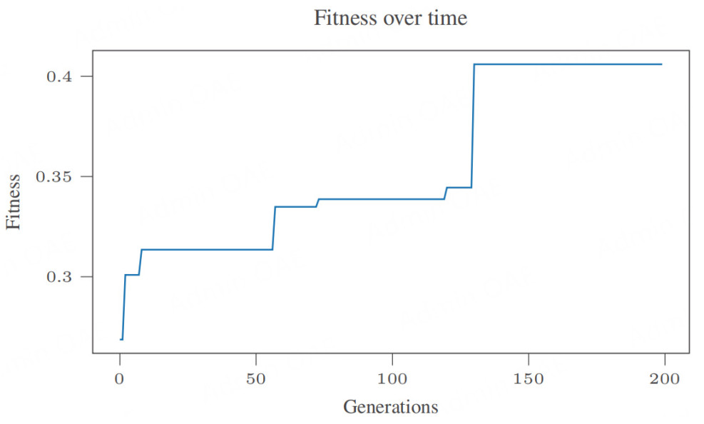
Figure 4. Convergence of the genetic algorithm.
3.2.2. Exploring fitness functions
Often, the fitness function for a GA is the inverse of the total error of the model being trained by the GA. In cases such as this, with such a high class imbalance, the model achieves a high overall accuracy, but fails to classify any points from the smaller class. To perform a systematic test on training performance measures, the GA was trained using three measures: log loss, area under the receiver operator curve (AUC), and APS (Average precision score summarizes the precision-recall curve as the weighted mean of precisions achieved at different thresholds, with the increase in recall from the previous threshold used as the weight. In other words, it measures how well a model can identify positive instances among all instances it predicts as positive, considering the varying thresholds. This makes it a useful metric for assessing models where precision and recall are crucial). Each measure was used as the singular fitness function for the GA, and then in combination with the other measures at various levels. The results are shown in Figure 5. Due to the societal cost of missing a dismantled ship (dismantled ships have the potential to be illegally beached), recall is a measure just as important as accuracy, if not more, as discussed in more detail in Section 4.3. To be clear, the class imbalance is one dismantled ship for every nine non-dismantled ships. If the model predicted every ship to be non-dismantled, it would achieve an accuracy of about 89%, but an APS and recall of 0%. The goal of the model is to catch the dismantled ships; thus, accuracy is far less meaningful for this task than APS. Accordingly, Figure 5A shows the performance achieved by the models trained on the various measures for an average of accuracy and recall. Figure 5B shows the performance of these models given by the APS, as this measure is more robust to imbalanced data compared to the standard AUC score[46]. Because the HFRBM outputs a prediction between 0 and 1, but class labels are needed, and Class 1is more important, the area under the APS is the best measure for the success of the HFRBM. Class 1denotes a ship that is at the end of its life, and class 0 denotes a ship that is not.
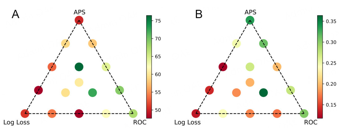
Figure 5. Performance evaluation of the model trained using the GA fitness functions tested. (A) average of accuracy and recall; (B) average precision score.
From Figure 5B, the best five fitness functions were chosen to train the HFRBM on all five folds of the data. The precision recall curve of the average results over the folds is given in Figure 6, where the legend denotes [weight of AUC, weight of APS, weight of Log Loss]. The 'best' of these fitness functions is subjective and depends on the performance measure(s) one hopes to optimize for. Log Loss does not perform well in either case, and taking the average of accuracy and recall does not perform well enough on APS. In this case, where catching the ships that are at the end of their life (class 1) is the main goal, the fitness function [0, 1, 0] that optimizes only for the APS was chosen.
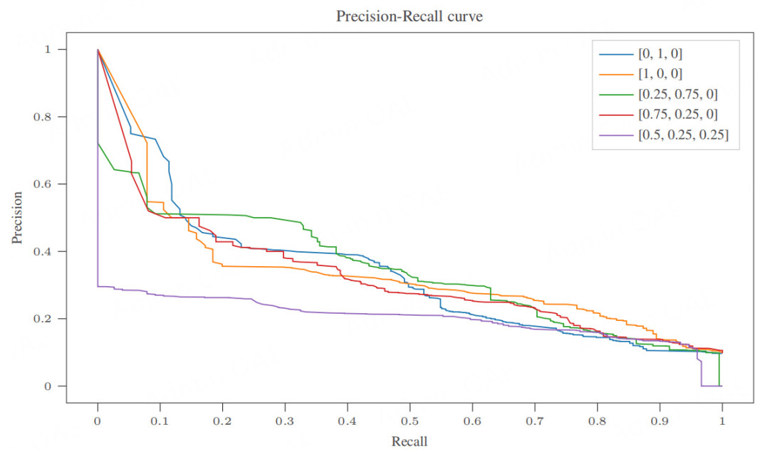
Figure 6. Average over five folds: model performance comparison of the models trained using the best GA fitness functions tested. The legend denotes [weight of AUC, weight of APS, weight of Log Loss].
4. PERFORMANCE OF THE HFRBM
It is a widely held belief among machine learning researchers that interpretability comes at the cost of a model's performance, although some researchers disagree[2]. The performance of the HFRBM developed in this paper is compared and discussed alongside two other models trained on the same dataset: a DT and a RF model.
4.1. Experimental set-up
The DT is an interesting model to compare the HFRBM with because it is commonly categorized as an intrinsically interpretable model[47]. The RF model is the best-performing model trained on the shipbreaking data by the ILT in prior work, and is an obvious baseline for comparison. Therefore, the FRBM is compared with a model categorized as intrinsically interpretable and another model with high accuracy.
The DT is built using the DecisionTreeClassifier from scikit-learn[48], which employs the Classification and Regression Trees method[49]. It is constrained to a depth of three, as this is the depth of the HFRBM structure. The DT classifier has a fixed depth of three and uses the Gini criterion to measure the quality of a split. The hyperparameters of the RF model are optimized through a grid search. The hyperparameters searched are the number of trees in the RF, the minimum number of samples required to be a leaf node, and the number of features to examine when considering the best split.
To more accurately represent the performance of the models, cross-validation is performed, where every time, a different subset of the data is used to train, and the remaining subset is used as a held-out test set. This is repeated five times (folds), with different subsets every time. The performance of the folds is then averaged to avoid any outlier performance due to the choice of the subset. The score used to train all the models is the APS.
4.2. Results
Table 2 presents the performance of each model. Accuracy is the percentage of data instances correctly classified. Recall is the proportion of actual positives correctly identified. For all the ships that are actually dismantled, the recall indicates the proportion correctly identified as dismantled. Precision measures the proportion of positive identifications actually correct, i.e., the ratio of true positives to all predicted positives. In this context, this corresponds to the number of broken ships correctly identified as broken, relative to all ships predicted as broken.
Average over 5 folds: score comparison across models
| Model | Random predictor | Random forest | Decision tree | FRBM |
| Accuracy | 51.23 | 94.46 | 90.49 | 48.68 |
| Recall | 47.87 | 57.98 | 34.42 | 79.23 |
| Precision | 9.69 | 80.20 | 52.04 | 14.16 |
| Avg precision score | 0.39 | 0.77 | 0.40 | 0.33 |
| AUC | 0.51 | 0.96 | 0.85 | 0.73 |
| Area under precision recall curve | 0.11 | 0.77 | 0.44 | 0.33 |
4.3. Discussion of results
In the shipbreaking application, correctly identifying the largest number of dismantled ships is a key objective. It is preferable for the model to flag these ships for further review than risk missing them. However, this objective must be balanced against the goal of reducing the number of ship inspections due to the constraint of having a limited number of ship inspectors. To achieve this balance, the focus is on the trade-off between recall and precision. Accordingly, Figure 7 highlights this metric rather than the more commonly used AUC score.
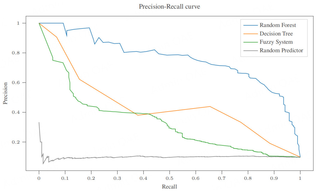
Figure 7. Average precision recall curves for all models.
Table 2 and Figure 7 are provided for completeness, but since this is a real-world application, it is useful to interpret the results in terms of actual inspections. The dataset contains about 2, 000 ships, collected over four years, corresponding to about 500 ships per year. Of these, 50 are dismantled annually. Inspecting ships scheduled for dismantling allows ship inspectors time to inform companies about ship recycling regulations and thereby prevent open-beach shipbreaking. The HFRBM model flags 280 of the 500 ships for inspection and successfully identifies 40 of the 50 dismantled ships. The RF flags 36 ships and captures 29 dismantled ships. Finally, the DT flags 33 ships and identifies 17 dismantled ships.
These results illustrate the explicit performance trade-offs involved in model selection. If there is sufficient capacity to inspect 280/500 ships, as recommended by the FRBM, this approach may be worthwhile to capture more dismantled ships. If inspection resources are more constrained, the RF model provides a more efficient option, maximizing the number of dismantled ships identified with fewer inspections. It is also important to note that performance is not the only consideration when choosing a model. In Section 5, the interpretability of these three models is further analyzed.
5. INTERPRETABILITY OF THE HFRBM
The primary goal of building a FRBM on the shipbreaking dataset was to build a model whose output can be understood by a non-technical end user. While difficult to do without a user study, an attempt is made in this section to analyze the extent to which that goal was achieved with the HFRBM. Additionally, the interpretability of the HFRBM is compared with that of the other models in this study, focusing on the information that model designers and model end users can extract. In the rest of the section, the models themselves are first visualized, and the level of interpretability and readability is analyzed without further intervention. Next SHAP is used to gain a local and then a global understanding of the models, making it possible to identify which features are most important and in what way they contribute to the model. This can support model end users in validating/identifying locally, unexpected or potentially false behavior, or to complement the information they already have. For model designers, it can provide global feedback about a model after a prediction has been validated, and a coherence check with the data being used. The SHAP waterfall plots and summary plots are employed to compare and discuss local and global interpretability of all three models.
5.1. Visualizing the models
To visualize the models themselves, a data point (data instance 44) that is correctly classified as a dismantled ship by all three models was chosen.
5.1.1. The hierarchical fuzzy rule-based model
A visualization of the FRBM is also developed to complement the raw rule outputs of the HFRBM, providing a higher level of insight in terms of interpretability than any other model. Figure 8A presents the trained input membership functions for the input Age in months as an example. As discussed in Section 3.1, these are SFPs to increase interpretability. Figure 9 displays a decision made by the trained HFRBM for data instance 44. Figure 10 visualizes the same decision, but starts deeper in the tree. The rules that describe this same visualization with words are shown in Table 3. They are broken down by the layer in which they are in the HFRBM. A total of 7 rules are needed to describe any one decision. Though readable, these rules are likely to be complex for non-technical end-users, and an interesting solution to this problem is introduced in Section 5.2.2. How to read these rules as a non-technical end user is also further discussed in the Supplementary Materials.
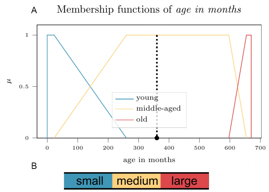
Figure 8. The Supplementary Materials for the FRBM visualization. (A) Trained input membership functions for the input Age in months of the ship. The star represents the value for ship age for data instance 44; (B) Standard color scale relating block color to membership function.
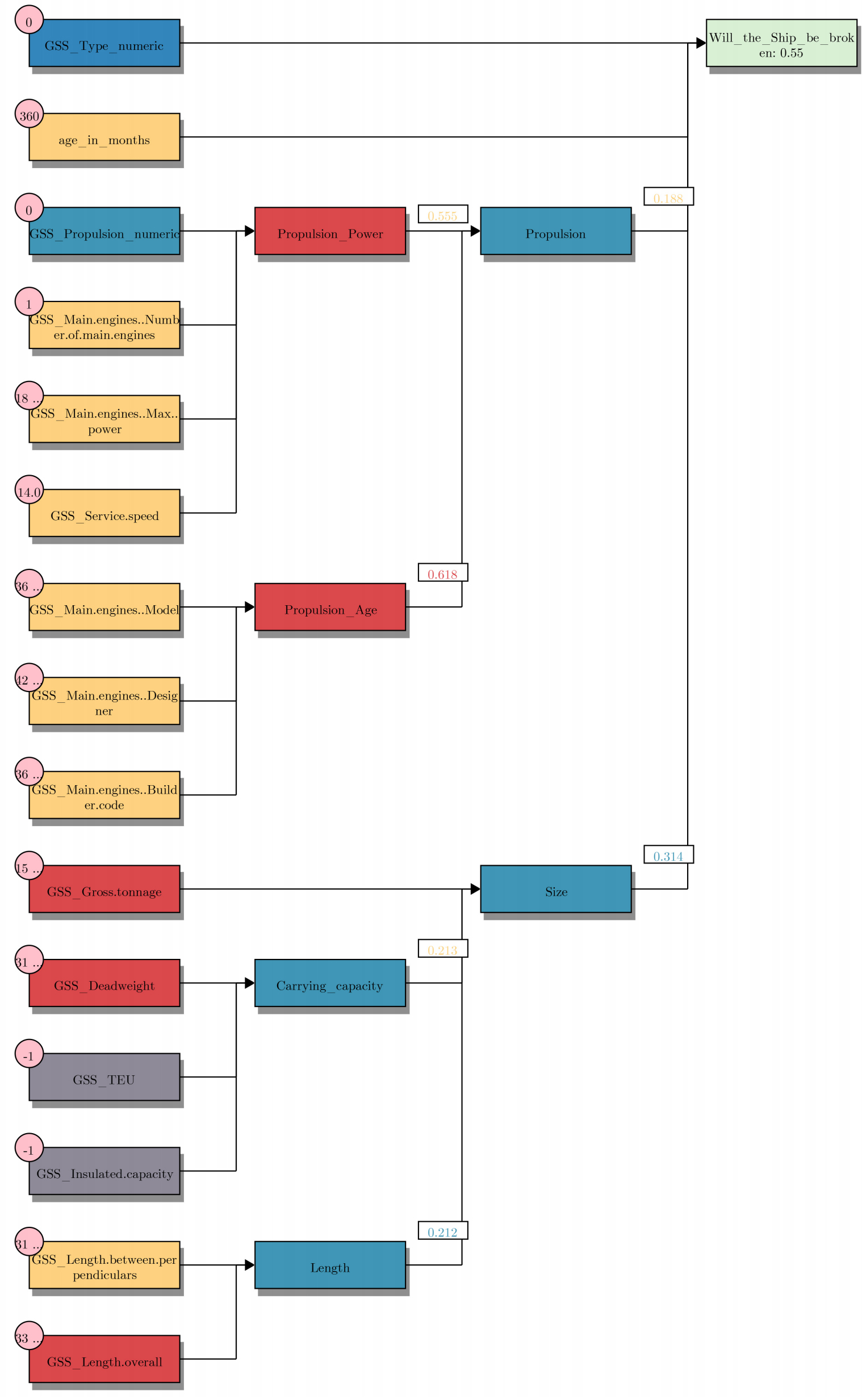
Figure 9. FRBM decision visualization for data instance 44.
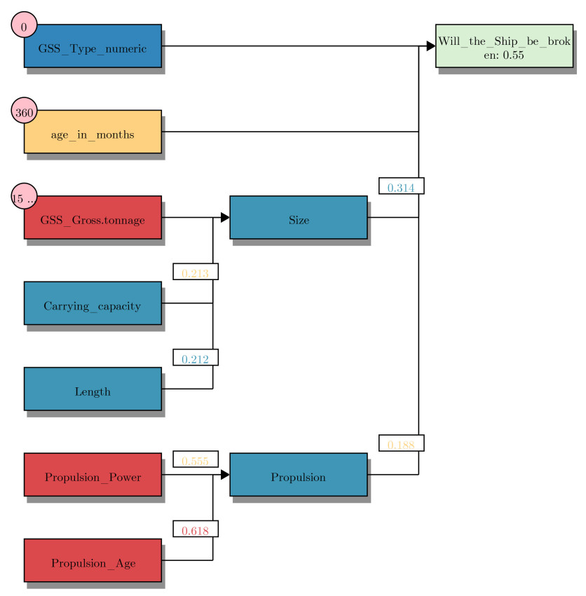
Figure 10. HFRBM decision visualization for data instance 44 without input layer. The input blocks are colored based on which input membership function is activated the most (low, medium or high), and the pink bubbles on the input blocks contain the actual feature value. The numbers exiting those input blocks represent the output value of the FRBM, and are colored based on which input membership function is activated in the next FRBM. These colors correspond to the color scale as seen in Figure 8B. The final output block is colored green if the prediction is correct, and red if the HFRBM prediction is incorrect. The darker the color, the more extreme the score is toward one of the two classes.
The rules that describe the FRBM decision for data point 44
| Rules |
| Input layer |
| If GSS propulsion numeric is type 0 and |
| GSS main engines number of main engines is medium and |
| GSS main engines max power is medium and |
| GSS service speed is medium then |
| Propulsion power is high |
| If GSS main engines Model is middle age parts and |
| GSS main engines designer is middle age parts and |
| GSS main engines builder code is middle age parts then |
| Propulsion age is high |
| If GSS deadweight is large and GSS TEU is not applicable and |
| GSS insulated capacity is not applicable then |
| Carrying capacity is low |
| If GSS length overall is large and |
| GSS length between perpendiculars is medium then |
| Length is low |
| Layer 1 |
| If GSS gross tonnage is large and Carrying capacity is medium and |
| Length is low then |
| Size is low |
| If propulsion power is medium and Propulsion age is high then |
| Propulsion is low |
| Final Layer |
| If GSS type numeric is type 0 and Age in months is middle age and |
| Size is low and Propulsion is medium then |
| Shipbreaking is high |
5.1.2. The decision tree model
The DT is shown in Figure 11.
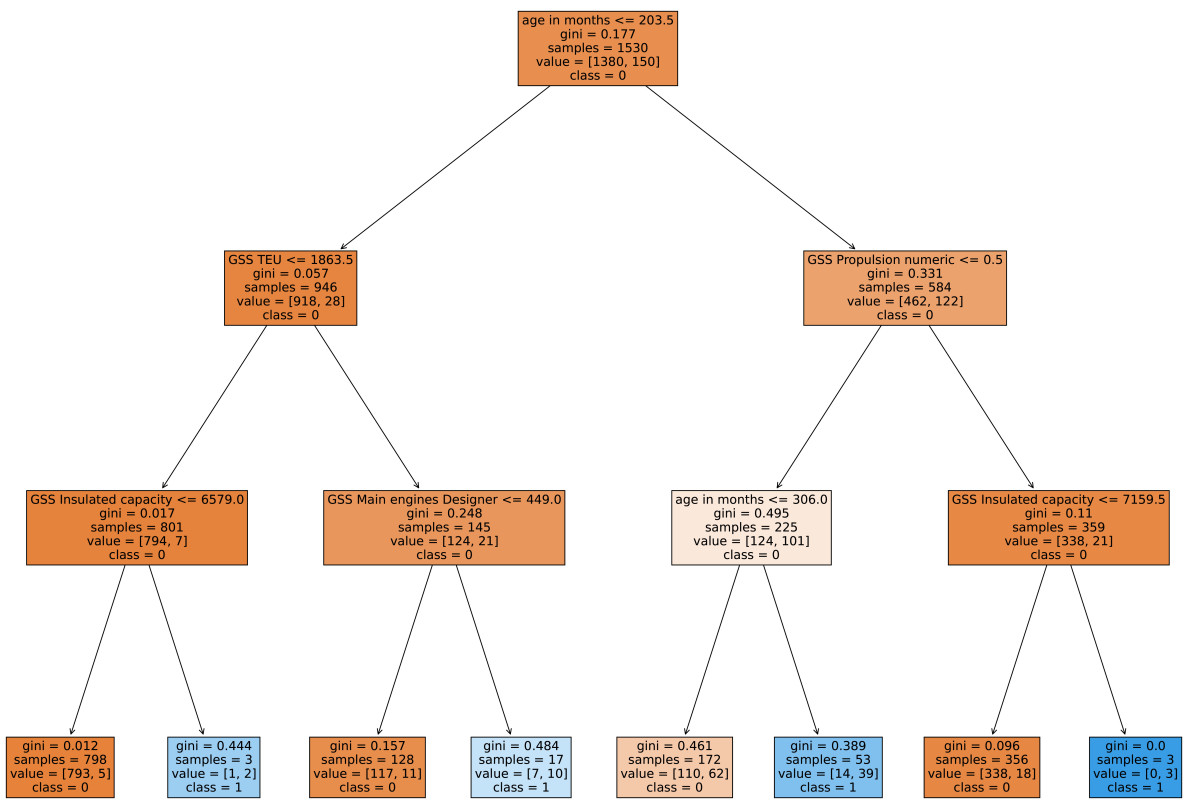
Figure 11. Trained decision tree model graph on one of the folds.
The rules that describe the DT are created with the help of[50], as shown in Table 4. The rules that activate to classify data instance 44 are highlighted in bold. As expected from a DT that is limited to a depth of three, the rule is very simple and does not take many of the input features into account.
The rules that describe the trained decision tree
| Rules |
| If (age in months <= 203.5) and (GSS TEU <= 1, 863.5) |
| and (GSS Insulated capacity <= 6,579.0) then class: 0 |
| (proba: 99.37%) | based on 798 samples |
| If (age in months > 203.5) and (GSS Propulsion numeric > 0.5) |
| and (GSS Insulated capacity <= 7, 159.5) then class: 0 |
| (proba: 94.94%) | based on 356 samples |
| If (age in months > 203.5) and (GSS Propulsion numeric <= 0.5) |
| and (Age in months <= 306.0) then class: 0 |
| (proba: 63.95%) | based on 172 samples |
| If (age in months <= 203.5) and (GSS TEU > 1, 863.5) |
| and (GSS Main engines Designer <= 449.0) then class: 0 |
| (proba: 91.41%) | based on 128 samples |
| If (age in months > 203.5) and (GSS Propulsion numeric <= 0.5) |
| and (Age in months > 306.0) then class: 1 |
| (proba: 73.58%) | based on 53 samples |
| If (age in months <= 203.5) and (GSS TEU > 1, 863.5) |
| and (GSS Main engines Designer > 449.0) then class: 1 |
| (proba: 58.82%) | based on 17 samples |
| If (age in months > 203.5) and (GSS Propulsion numeric > 0.5) |
| and (GSS Insulated capacity > 7,159.5) then class: 1 |
| (proba: 100.0%) | based on 3 samples |
| If (age in months <= 203.5) and (GSS TEU <= 1,863.5) |
| and (GSS Insulated capacity > 6,579.0) then class: 1 |
| (proba: 66.67%) | based on 3 samples |
5.1.3. The random forest model
Direct visualization of the RF model is not applicable in this context. The RF model does have internal feature importances, which are the impurity-based feature importances of the model. These feature importances are compared with those found by SHAP in one study[51]. The study uses feature importance determinations both to select a subset of features for model training and to evaluate the actual importance of these features based on the resulting change in performance. Their results vary across models, but overall, one method does not highly outperform the other. Therefore, and because there are no internal feature importances in the HFRBM, the post-hoc interpretability method SHAP is used to interpret all models in a similar manner.
5.2. Local interpretability
In Machine Learning, local interpretability represents the possibility of a human observer to understand a single model output. For this application, the question is: is a model designer and/or model end user able to understand why a certain ship was predicted to be dismantled?
5.2.1. Waterfall plot analysis
The SHAP waterfall plots in Figures 12, 13, 14 display the single decision taken by each of the three models for data instance 44. E[f(x)] is the baseline value, i.e., the average output for a model across all its training (background) points. A waterfall plot attempts to explain the difference between this base prediction,
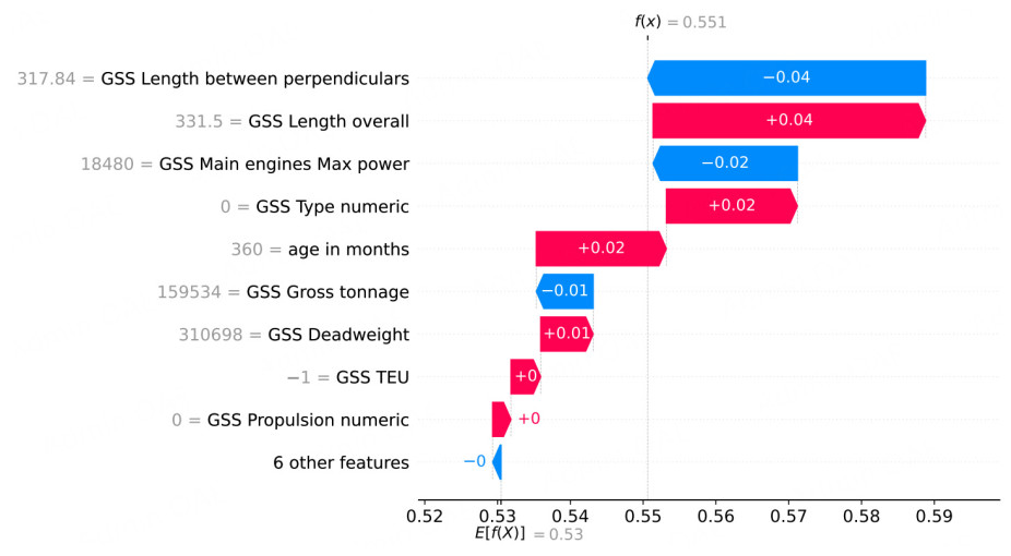
Figure 12. FRBM waterfall plot for data instance 44.
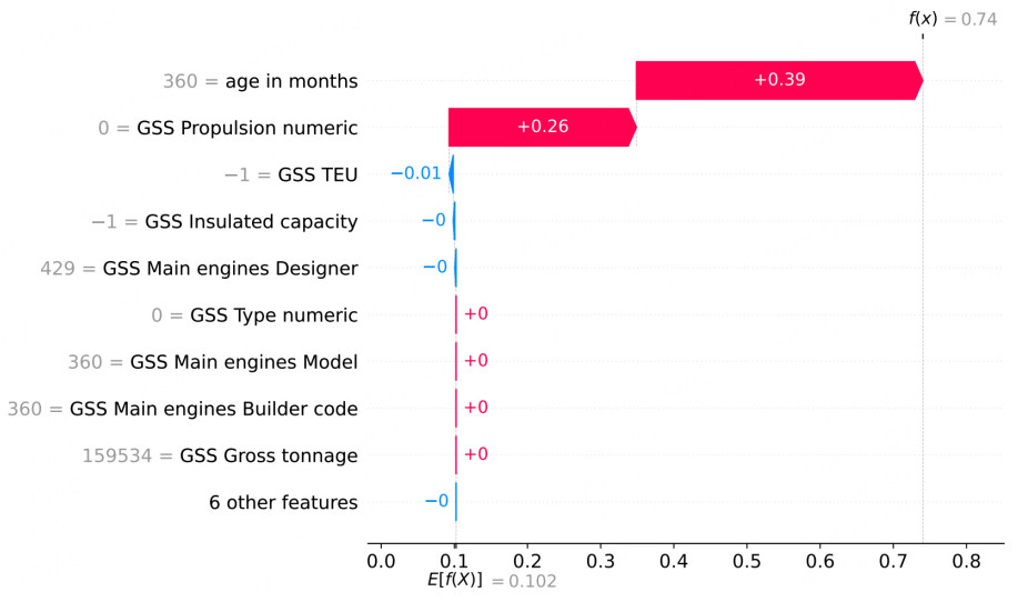
Figure 13. DT waterfall plot for data instance 44.
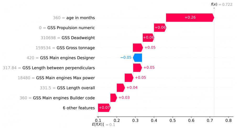
Figure 14. RF waterfall plot for data instance 44.
The waterfall plot for the DT [Figure 13] shows that, as expected, only three features contribute significantly to the final prediction, while in the RF model [Figure 14], all of the features influence the final output. The waterfall plot for the HFRBM [Figure 12] shows that 8/15 features have a significant impact on this particular decision.
5.2.2. Discussion
How can this post-hoc local interpretability analysis help model end users to understand and compare the models? Is it possible to achieve an understanding of how the RF model makes its decision, especially with no understanding of the model itself?
In Figure 13, the waterfall plot of the DT clearly shows what the rules are. It provides more information about the impact of Age in months compared to the GSS Propulsion numeric and GSS TEU. From Figure 13, it can be seen that Age in months has almost twice the impact on the output compared to GSS Propulsion numeric, and that Age in months has an almost 40 times greater impact on the output compared to GSS TEU. While some of this information could be partially inferred from the rules themselves, the visualization offers a clearer, more informative picture. The waterfall plot of the HFRBM does provide added information about the most important features. One way that a model designer may be able to make use of this added model interpretability is to reduce the rules given in Table 3 for presentation to the model end user. The waterfall plot shows which input features have little impact and can be removed from the rules, resulting in simple, yet informative rules, as shown in Table 5. For this example, according to SHAP, the rules shown account for 97% of the decision made. This percentage is calculated by summing the absolute SHAP values for all input features for a given decision, then comparing the sum of the remaining features after removing the least important ones to the full sum. Eliminating features with zero or near-zero impact yields the 97% coverage. The user can further reduce the rules to any given percentage, depending on the model end user preferences, such as 85% in Table 6. This approach reduces the number of rules without simplifying the model itself, while still enhancing the end user's understanding of the decision process.
The rules that describe the FRBM decision for data point 44, reduced by SHAP importance in waterfall plot, accounting for 97% of the decision made
| Rules |
| Input layer |
| If GSS deadweight is large and GSS TEU is missing then |
| Carrying capacity is low |
| If GSS length overall is large and |
| GSS length between perpendiculars is medium then |
| Length is low |
| Layer 1 |
| If GSS gross tonnage is large and Carrying capacity is medium and |
| Length is low then |
| Size is low |
| Final layer |
| If GSS type numeric is type 0 and Age in months is middle age and |
| Size is low and GSS main engines max power is medium then |
| Shipbreaking is high |
The rules that describe the FRBM decision for data point 44, reduced by SHAP importance in waterfall plot, accounting for 85% of the decision made
| Rules |
| Input layer |
| If GSS length overall is large and |
| GSS length between perpendiculars is medium then |
| Length is low |
| Final layer |
| If GSS type numeric is type 0 and Age in months is middle age and |
| Length is low and GSS main engines max power is medium then |
| Shipbreaking is high |
As the most complex model analyzed in this work, the RF benefits most from post-hoc interpretation methods; these methods provide the greatest insight. Examining the RF waterfall plot in Figure 14, it can be seen that Age in months is the most important input for this decision. However, the rest of the features have similar contributions, and thus, a model designer gains minimal added value from using the SHAP waterfall plot. As mentioned above, a model end user would be unlikely to consult waterfall plots at all.
5.3. Global interpretability
Global interpretability can be viewed as the ability of a target human audience to understand the model as a whole. In this application, is a target audience able to understand in general why ships are dismantled or not, according to a certain model? The target audience for global interpretability for this application is primarily the model designer; however, the end user may be provided with global interpretability tools when first introduced to a new model, offering context for how best to use the model. SHAP summary plots are used as the initial global interpretability tool. Figures 15, 16, 17 provide the violin plots for the HFRBM, DT, and RF models, respectively. Due to the difference in distribution in the test sets considered for each of the folds during the cross-validation, the violin plots for each model vary across the folds described in Section 3.2. Therefore, the violin plot for folds 0 and 1 for each model is shown. The remaining folds are given in the Supplementary Materials.
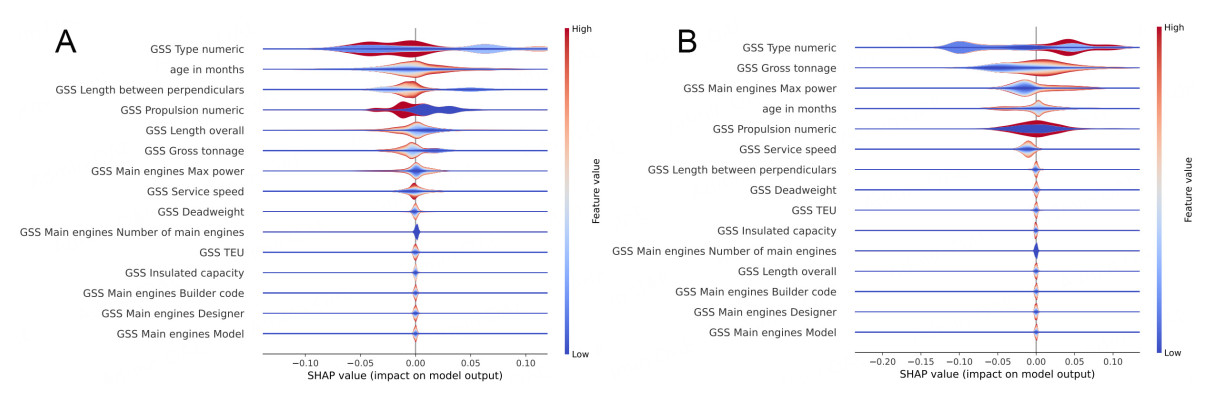
Figure 15. HFRBM violin plot for folds 0 and 1. For each test point assessed, the impact of the individual features from SHAP, and the value of the feature from the data set are given. The violin plot stacks these points, grouping those with the same SHAP value, and coloring the grouped points by the feature value. In this way, an understanding of how each feature affects the model globally is gained. (A) HFRBM violin plot for fold 0; (B) HFRBM violin plot for fold 1.
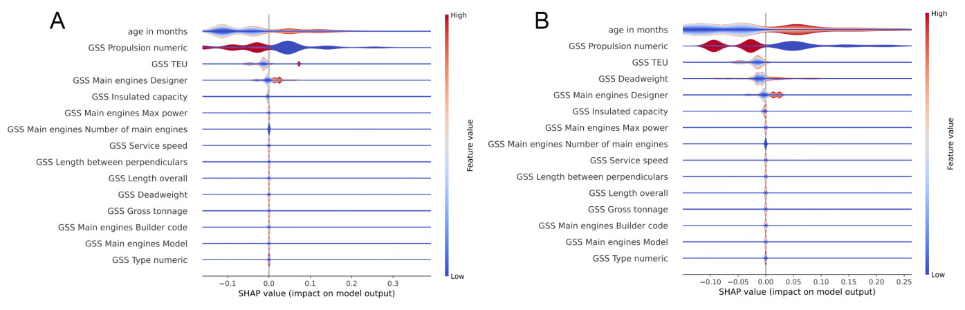
Figure 16. Decision Tree violin plot for folds 0 and 1. (A) DT violin plot for fold 0; (B) DT violin plot for fold 1.
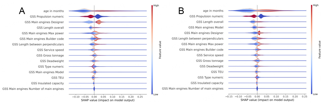
Figure 17. Random forest violin plot for folds 0 and 1. (A) RF violin plot for fold 0; (B) RF violin plot for fold 1.
5.3.1. Violin plot analysis
In the HFRBM violin plots [Figure 15], GSS Propulsion numeric influences the model (for fold 0) in a manner similar to that observed in the DT and RF models, which is expected because this feature is a categorical variable. The HFRBM for fold 1 does not show this same pattern. Additionally, most other features have a less clear and distinguishable impact on the model, indicating that the model does not use those features in a straightforward way to distinguish between the two classes. Nonetheless, the model designer can still glean information about the most important features, and some basic patterns that show how those features affect the model output. For example, it is observed that a higher Age in months for both folds causes a slightly more positive SHAP value, on average. Some lower ages also correspond to a positive SHAP value (the dark blue line through the center of the Age in months violin bar). Furthermore, GSS Type numeric is a categorical feature, so it is logical that there are clear groupings (strong colors together) and that the assigned numeric category does not lend to a clear division between the high and low feature values.
The plots in Figure 16 for the DT model show what may be gleaned from the rules in Section 5.1.2: only five of the input features influence the output. It can be easily seen that a higher Age in months and a lower GSS Propulsion numeric have an impact in pushing the output to the positive class. The impact of the other three features is not quite as clear. Higher GSS TEU and GSS main engines designer have an impact in pushing the output to the positive class for a smaller number of data points, but the full effect cannot be distilled by this visualization or method alone. Across the two folds shown for the DT, the effect of the features appears to be very consistent, though the shape of the exact effect changes.
The RF violin plot [Figure 17] shows that all inputs other than GSS main engines number of main engines have a global impact on the output of the model. As shown in Section 5.2, interpretability is not found in the model itself or at the local level of the RF model for the model designer or the model end user. This violin plot gives the model designer a first insight into how the model makes decisions on a global level, and what features are the most important. Just as for the DT, the impact of the features across the folds is quite consistent, though there are changes in the order of the most important features. Across the folds, consistent patterns are observed in the violin plots for feature values and SHAP values. However, the overall shape of the violin plot varies, which indicates differences in the distribution of SHAP values across features. This is especially so with GSS Main engine designer. For both folds, a low value of GSS Main engine designer corresponds to a negative SHAP value, while a high value of this feature corresponds to a positive SHAP value. However, the shape of the violin changes significantly across the folds, so caution must be exercised not to draw many conclusions from the exact shape of the violin plot for this model. For the further analysis that the model designer will conduct, a different view of this global interpretability data is examined.
5.3.2. Dependence plot analysis
It is instructive to compare the SHAP violin plots of the HFRBM with those of the RF as model designers, to gain insights into what accounts for the differences in what the models have learned. This is particularly relevant if the goal of this work is to build a model that can accurately identify a small number of ships for inspection (a current strength of RF model) while still detecting a large number of dismantled ships (a current strength of the HFRBM model). To investigate this, the violin plots in Figures 15 and 17 are examined, alongside the SHAP dependence plots. The SHAP dependence plot visualizes the value of an input compared to the SHAP value of that input feature, per data point. A trend observed in the dependence plot reveals more detailed effects of an input on the model's output.
Both models agree that Age in months is very important, though the RF model has it as the most important, and the HFRBM has it as the second most important across the folds. A comparison of the dependence plots of this input feature across the two models, as given in Figure 18, illustrates some similarities and differences. The dependence plots are plotted by combining all the fold results, but the individual fold dependence plots are provided in the Supplementary Materials because there are differences across the folds, especially for the HFRBM. For both models, an age of 200 months shows to be an inflection point. For the RF model, ages above 200 months correspond to positive SHAP values, and those below correspond to negative SHAP values. For the HFRBM, the pattern is less clear. For ages below 200, there are positive and negative SHAP values, which are difficult to understand in just this plot. Figure 19A and B, discussed in the next paragraph, further illustrates this trend. For ages above 200 months, the SHAP values are generally close to 0 and more positive, though a line of low SHAP values is also observed, which gains more context when examining Figure 19B. Overall, it is learned that 200 months is a discriminatory age, and that the age-model output relationship is far more complex for the HFRBM, likely depending on other variables, than the age-model output relationship for the RF. Indeed, analysis of the dataset shows that 82% of the dismantled ships are above the age of 200 months, supporting this pattern. To explore the potential influence of these other variables, the same figures are plotted while coloring them according to the value of a third variable. In this case, GSS Propulsion numeric is used, a key feature in both models. In both Figure 19B (HFRBM) and Figure 19A for (RF), clear patterns emerge from the interaction with GSS Propulsion numeric.
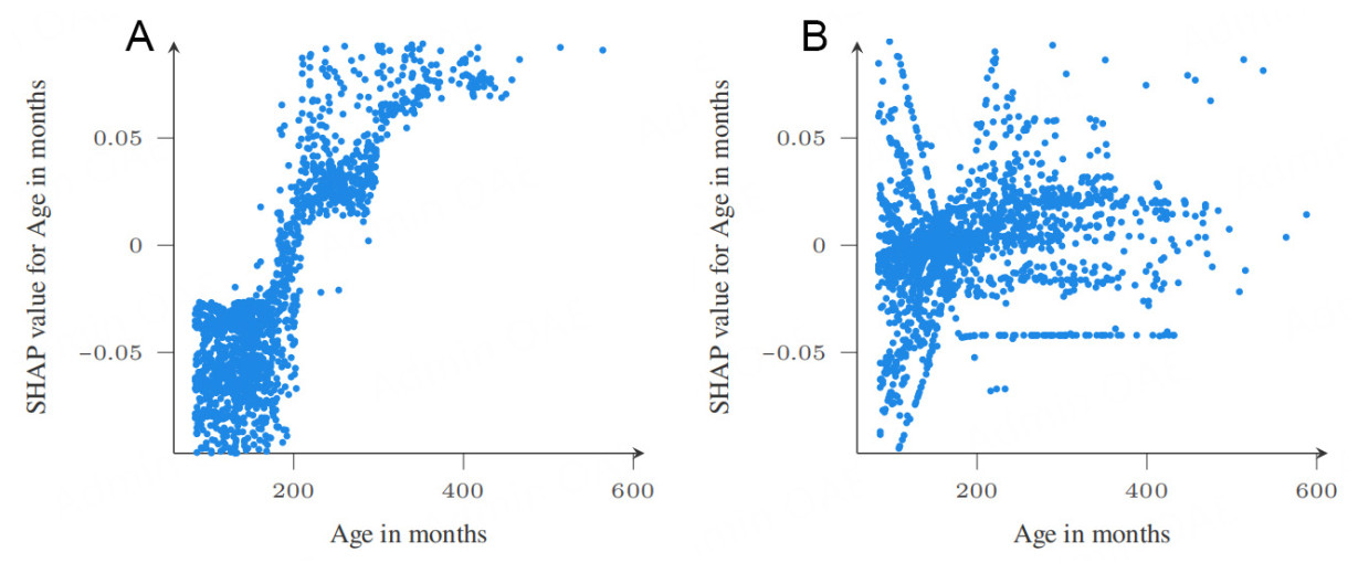
Figure 18. Age in months dependence plot RF - HFRBM comparison for all folds. (A) RF age in months SHAP dependence plot; (B) FRBM age in months SHAP dependence plot.
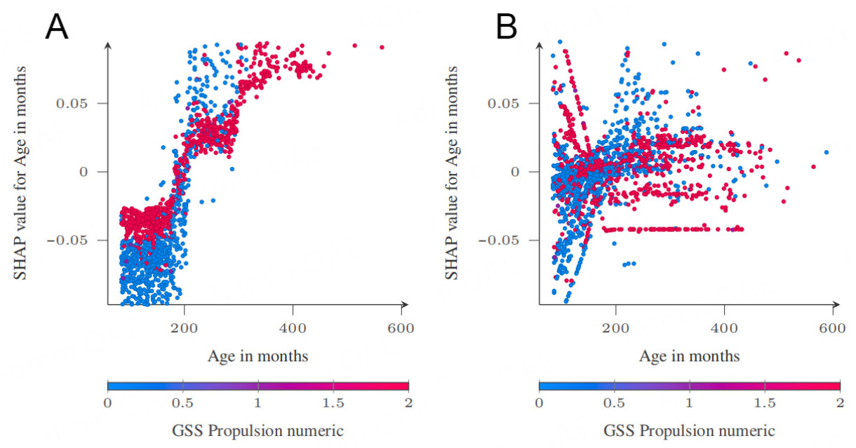
Figure 19. Age in months dependence plot RF-FRBM comparison with GSS propulsion numeric interaction coloring for all folds. (A) RF age in months SHAP dependence plot; (B) FRBM age in months SHAP dependence plot.
This is an especially useful insight for the model designers of the HFRBM. It appears that when GSS Propulsion numeric is category 0, the trend in the figure is closer to the trend in the figure for the RF model. When GSS Propulsion numeric is category 2 in the HFRBM, the SHAP value of Age in months decreases as Age in months increases. This trend is the reverse of the pattern observed in the plot when GSS Propulsion numeric is category 0. This is easily stated as a rule, because this is part of the rules in the model. If the model designers believe this is a pattern that the HFRBM has falsely learned, this rule can be found in the HFRBM, and edited to be more in line with how this model would be expected to work. This once again shows the strength of the HFRBM, and gives an interesting example of how a post-hoc interpretability method, such as SHAP, can be useful.
Figure 20 presents a dependence plot comparison for the input feature GSS type numeric, or ship type. This feature is the focus because it ranks highest in importance for the HFRBM, and is the fifth least important for the RF model. As shown in Figure 20, the scale of SHAP impact for the RF is, on average, less than half that of the HFRBM. In the RF model [Figure 20A], most ship types have minimal influence on class prediction, except for type 0 (bulk carrier), which pushes predictions toward class 1. In contrast, for the HFRBM, four out of eight ship types exhibit a more distinct influence on class assignment. Specifically, types 0 and 4 in the RF model push toward class 1, whereas in the HFRBM, these types have a more balanced effect and do not favor a particular class. Conversely, type 2 pushes toward class 1 in the HFRBM but shows a balanced effect in the RF model.
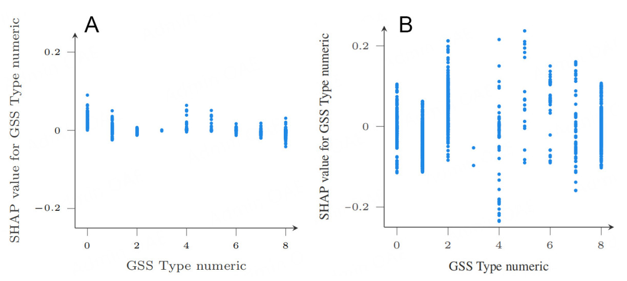
Figure 20. GSS type numeric dependence plot RF-HFRBM comparison for all folds. (A) RF GSS type numeric SHAP dependence plot; (B) FRBM GSS type numeric SHAP dependence plot.
5.3.3. Global interpretability discussion
Overall, it appears that the hierarchy chosen for the HFRBM has some priority over marginal contributions as measured by SHAP. Table 7 presents the most important features as identified by SHAP values, averaged over all the folds. The features are colored to match the FRBM that they first enter, matching the HFRBM structure given in Figure 3. It is observed that the two inputs that directly enter the final FRBM, GSS type numeric and Age in months, are the two most important features. Notably, GSS type numeric is a very unimportant feature for the RF model. The other feature, GSS gross tonnage, which passes through only one FRBM before entering the final FRBM, is the fourth most important feature. It is hypothesized that when the features that have a direct connection with the final FRBM are removed, there is an immediate effect on the output. However, other features that go through two intermediate FRBMs first likely have a more attenuated effect when "removed". By design, these inputs first feed intermediate FRBMs, whose outputs then propagate to the next layer, making the influence of such inputs less direct. Although this analysis is limited to one dataset, and one method of feature importance calculation, and further tests need to be conducted, it suggests an important consideration for the design of HFRBMs for interpretability in the future. Model designers need to account for the semantic relevance of intermediate FRBMs within the context of the data[10] and consider that the distance of an input from the final FRBM - in terms of "layers" - may affect its influence on the output.
The top features for the HFRBM across all folds. The colors match the FRBM hierarchy shown in Figure 3 in which the inputs are colored and grouped according to the intermediate FRBMs they feed into
| Color in HFRBM structure | Ordered Top features | # FRBMs between input and final FRBM |
| 1 | GSS Type numeric | 0 |
| 2 | Age in months | 0 |
| 3 | GSS Propulsion numeric | 2 |
| 4 | GSS Gross tonnage | 1 |
| 5 | GSS Main engines Max power | 2 |
| 6 | GSS TEU | 2 |
| 7 | GSS Length between perpendiculars | 2 |
| 8 | GSS Length overall | 2 |
| 9 | GSS Service speed | 2 |
| 10 | GSS Deadweight | 2 |
| 11 | GSS Main engines Designer | 2 |
| 12 | GSS Main engines Number of main engines | 2 |
| 13 | GSS Main engines Builder code | 2 |
| 14 | GSS Insulated capacity | 2 |
| 15 | GSS Main engines Model | 2 |
Having examined global interpretability, the value added by this SHAP analysis is reflected upon. It was found that visualizing the HFRBM itself provides more informative insights than the SHAP waterfall plot. Nevertheless, the waterfall plot can help minimize the number of rules, thereby enhancing HFRBM interpretability. The violin summary plot offers limited insight because most feature–output interactions are multidimensional. However, it serves as a useful starting point for generating dependence plots, which capture subgroup heterogeneity and homogeneity - arguably the most informative plots for this study. While dependence plots are not directly useful for model end users, they can guide model designers in formulating some approximate global rules or refining rules learned by the model.
Finally, the interpretability and performance of each model are briefly summarized in Table 8. In this way, the performance and interpretability of each model can be compared. It is very difficult to measure the interpretability without an actual user study, so the interpretability analysis in the table contains the highlights from each deeper analysis performed in the previous sections of this paper.
Interpretability-performance overview
| Model | Random forest | Decision tree | FRBM |
| Accuracy | 94.46 | 90.49 | 48.68 |
| Recall | 57.98 | 34.42 | 79.23 |
| Model visualization | Model is too large | Possible | Possible; innovative technique |
| Model local interpretability | SHAP shows the most important feature and does not distinguish between other features | SHAP adds valuable information | SHAP reduces model rules to improve interpretability |
| Model global interpretability | Feature importances are useful to the model designer | Feature importances are useful to the model designer | Helps the model designer identify an important relationship between the hierarchy and variable importance that may be undesired |
6. DISCUSSION
Two relevant challenges to the HFRBM model trained in this work are discussed. The first challenge is created by the simplification of the real-world data so that a model can be trained on it. The second challenge briefly discussed is the absence of monotonicity with respect to the age of a ship.
6.1 Time challenge
The obvious challenge to applying the trained HFRBM created here is the low accuracy, even if that is not the most important performance measure in this work. This limitation largely stems from the nature of real-world, unbalanced data sets such as the one used in this work. A RF model, which is often trained on "toy" data sets with accuracies over 99%, achieves 94.4% accuracy on this data set, although the more meaningful value for such an unbalanced data set is the APS, which in this case is 0.77. To apply machine learning models for real-world applications, the data must be simplified. One such simplification in this study was the removal of the temporal dimension, reframing the task as a static classification problem. Yet, the dismantlement of a ship is inherently time-dependent. In the current classification formulation, the model is asked to determine, at a specific month, whether a ship is dismantled or not. The month before dismantlement, the ship is classified as "not dismantled". This temporal sensitivity makes the task particularly demanding, especially when combined with the imbalance of the dataset.
To address this, a test was conducted to reintroduce temporal information into the problem. Specifically, the ships in the test data sets were duplicated and only the time-dependent inputs were modified at defined intervals. The model then produced predictions across these intervals, and the predictions were weighted before being combined into a final prediction. The most effective weighting methods were simple averaging and taking the maximum, although other methods were also evaluated. Table 9 summarizes the results. The time intervals tested were 10 years (± 5 years on either side of the ship age) and 4 years (± 2 years). While more time intervals should be tested in future work, and temporal information should be included in the training of the model as well, these intervals were sufficient to provide a preliminary evaluation. For both models, the best results under each weighting method are reported relative to the original model results. The HFRBM achieved higher accuracy and recall by taking the average prediction over a period of 10 (± 5) years. The model achieved even higher recall using the maximum over a 4-year (± 2) interval; however, the accuracy decreases. The RF model also showed higher recall when taking the maximum over 10 (± 5) years with a decrease in accuracy, though it did not achieve the recall of the HFRBM.
The time interval test for the HFRBM and RF
| Time (±) year | Weights | Accuracy | Recall | Precision |
| Hierarchical fuzzy rule-based model | ||||
| 0 | None | 49.18 | 75.99 | 15.13 |
| 2 | Max | 37.34 | 94.74 | 13.14 |
| 5 | Average | 51.17 | 84.21 | 15.02 |
| Random forest model | ||||
| 0 | None | 93.19 | 51.35 | 70.37 |
| 2 | Average | 93.46 | 48.65 | 75 |
| 5 | Max | 87.43 | 67.57 | 40.98 |
These findings suggest that reintroducing temporal information into the dataset improves the performance of both models. More broadly, this highlights the importance of recognizing the limitations imposed by simplifying real-world data for modeling. For interpretable model development, a critical task of the model designer is to carefully analyze these limitations and document their implications.
6.2. Monotonicity challenge
Monotonicity is an interpretability constraint that ensures, for example, that as a feature increases, the corresponding output either consistently increases or consistently decreases. Such a relationship is not necessarily present in practice. However, in the design of interpretable models, monotonicity that reflects structural knowledge of a problem domain is a useful constraint that model designers must apply whenever possible.
Consider the case of ship dismantlement. As highlighted by the global SHAP analysis in Section 5.3), age is a critical factor in determining whether a ship is dismantled. In fact, the relationship between age and dismantlement could be a prime example of the constraint of monotonicity: if all other features of a ship remain constant while its age increases, one would reasonably expect the predicted probability of dismantlement to stay the same or increase, but certainly not decrease. However, the situation is more nuanced. Domain experts have observed that ships reaching a certain age may actually continue in service for a long time, breaking the expected monotone pattern. If model end users assume a monotonic relationship that the model does not reflect, this can create confusion and mistrust. Therefore, model designers must carefully consider how monotonicity constraints are applied and clearly communicate their implications when presenting models to model end users.
7. CONTRIBUTIONS AND CONCLUSIONS
In the Netherlands, there are only 20 ship inspectors and tens of thousands of ships entering each year. Given that an interpretable machine learning model can be a decision tool for ship inspectors to more efficiently prioritize ships for inspection, a HFRBM trained by a GA was presented as a more interpretable model than a RF model. The type of audience is important in any consideration or evaluation of interpretability. The focus was on two audiences in this work. The ship inspectors, or the model end users, are the ultimate beneficiaries of this interpretable model. However, interpretability aimed at the model designers is also important in this work to help create interpretability for the model end users. The various performance metrics and trade-offs as they relate to the ship-dismantling application were thoroughly discussed, and it was found that the HFRBM flags more ships for inspection, but also identifies more of the dismantled ships. The interpretability of the HFRBM was demonstrated using tools built from the model itself, and then a feature importance method SHAP was employed to gain additional interpretability insights. A method was proposed to use local SHAP to reduce the rules shown to a model end user while maintaining full coverage of the input space and without reducing the rules in the model itself. Global SHAP explanations, on the other hand, provided model interpretability for the model designer. These results showed that the features most influential in the HFRBM predictions are the same as those that directly contribute to the final FRBM. In other words, the structure of the chosen hierarchy seemed to strongly influence feature importance as revealed by SHAP.
The trade-off between interpretability and performance was examined and presented. Ultimately, the 'best' model for this real-world problem relies on balancing model interpretability, population size constraints, available capacity, and model performance.
There are many avenues of future work that could be explored. The first is to expand the HFRBM to apply it to the shipbeaching problem, and to achieve a better performance in training the HFRBM on both the shipbreaking problem described in this work and the shipbeaching problem. This could involve investigations into multi-objective fitness functions for the GA in training the HFRBM. To further improve the interpretability of the HFRBM, it would be possible to build on this work by eliminating the least important features according to the global SHAP analysis, and iteratively train new models. Fewer inputs make it easier for a human to interpret the output of the model. Rule-reduction methods could also be investigated to remove potentially redundant, erroneous, or conflicting rules[52]. SHAP could potentially serve as an additional method for rule reduction, complementing previously used methods. Another promising direction is to study how the HFRBM's architecture affects both outputs and feature importance. The same theory would be applied to a different dataset - one with a similar number of inputs but a more balanced output distribution - to test this hypothesis. However, for all of these works, the imbalance of the dataset looms as a large challenge. Moreover, the temporal aspect of the dataset, as discussed only briefly here, may require an entirely new data collection approach spanning many years before it can be fully addressed.
The purpose of any model built for this application is to provide a decision support tool for ship inspectors, or those authorities deciding which ships should be inspected. Although much more research is required, such a tool could prove highly valuable. In particular, a system that helps inspectors schedule inspections of ships that are deemed to be at higher risk of illegal beaching practices would be especially helpful given the limited number of ship inspectors. However, due to the high-risk nature of such an application and the government's responsibilities to its citizens, such a tool must be carefully evaluated before deployment.
While an attempt has been made to comment on visualizing and understanding the models tested, as well as the local and global interpretability, to truly test these aspects of a model, user studies should be conducted in two phases. The first phase must focus on presenting data in a non-misleading and understandable way, such as through an interactive dashboard. User interface design and testing will be key in this phase. The user tests will test for ease of use, inspectors' understanding of model decisions, and perhaps most importantly, the independence of the ship inspectors. Independence here refers to inspectors' ability to override the model when they believe it to be incorrect, which is crucial in maintaining human oversight in such a system. It is easy for humans to become over-reliant upon such a model to make decisions, and this is dangerous. While a difficult task, inspiration from phishing test emails may be drawn. Companies send simulated phishing emails to their employees so that their employees are trained to detect and report scam emails. Incorporating a similar approach into this decision support system can keep users alert and offer model designers a metric of how alert the users are to these simulated incorrect decisions of the model.
The second phase of this user study would assess the actual impact of the tool on human decision making. A controlled experiment would be designed, where a group of ship inspectors would use the tool after training, while the control group of ship inspectors would continue their work without it. The key performance indicators in this controlled experiment would include the time needed by an inspector to make a decision and the accuracy of identifying high-risk ships. This would allow for a determination of whether inspectors equipped with the tool perform their tasks more effectively.
DECLARATIONS
Acknowledgments
The authors gratefully acknowledge Antonio Pereira Barata from the ILT for his help with the experimental setup suggestions for assessing model performance. Sincere appreciation is also extended to the anonymous reviewers for their insightful comments and constructive feedback, which have significantly improved the quality of this paper.
Authors' contributions
Made substantial contributions to the conception and design of the study, carried out the study, performed data analysis, interpretation, and wrote the majority of the original draft: Pickering, L.
Contributed to the conception and design of the study, performed data acquisition, provided administrative, technical, and material support, and performed writing and editing: Ciulei, V.; Merkx, P.
Contributed to the conception of the study, provided administrative and material support, and performed writing and editing: van Vliet, J.
Contributed to the conception and design of the study, and performed editing: Cohen, K.
Availability of data and materials
The dataset is provided by the ILT. The data cannot be shared because it contains information that is not publicly available. The following three sources have been used to create the data: 1. Open data from the NGO Shipbreaking Platform[32] and available to the public; 2. Data from the Global Integrated Shipping Information System (GISIS)[33], only accessible with an official account; and 3. Data of port calls from the information system of THETIS-EU of the EMSA[34], only accessible with an official account.
Financial support and sponsorship
While performing this work, in two separate time periods, the first author was a recipient of a Fellowship of the Belgian American Educational Foundation (https://baef.be/fellowships-for-americans/) and a Fulbright Ghent University Award (https://us.fulbrightonline.org/fulbright-us-student-program). These awards supported Lynn Pickering in experiment design, analysis and interpretation of data, and the writing of the manuscript.
Conflicts ofinterest
Cohen, K. is Subject Editor of the journal Complex Engineering Systems and Guest Editor for the topic "Explainable AI Engineering Applications" in this journal. Cohen, K. was not involved in any steps of editorial processing, notably including reviewer selection, manuscript handling, or decision making; Ciulei, V.; Merkx, P.; van Vliet, J. are all affiliated with the Inspectie Leefomgeving en Transport (ILT), They declared that there are no conflicts of interest in relation to the work carried out as part of the submission; Pickering, L. declares that there are no conflicts of interest.
Ethical approval and consent to participate
Not applicable.
Consent for publication
Not applicable.
Copyright
© The Author(s) 2025.
REFERENCES
1. European Union. Proposal for a regulation of the European Parliament and of the council laying down harmonised rules on artificial intelligence (artificial intelligence act) and amending certain union legislative acts; 2021. Available from: https://eur-lex.europa.eu/legal-content/EN/ALL/?uri=celex:52021PC0206#document2 [Last accessed on 31 Oct 2025].
2. Rudin, C. Stop explaining black box machine learning models for high stakes decisions and use interpretable models instead. Nat. Mach. Intell. 2019, 1, 206-15.
4. Alonso, J. M.; Magdalena, L. Special issue on interpretable fuzzy systems. Inf. Sci. 2011, 10, 4331-39.
5. Alonso Moral, J. M.; Castiello, C.; Magdalena, L.; Mencar, C. Designing interpretable fuzzy systems. In: Explainable fuzzy systems, studies in computational intelligence. Cham: Springer International Publishing; 2021. pp. 119-68.
6. Alonso Moral, J. M.; Castiello, C.; Magdalena, L.; Mencar, C. Design and validation of an explainable fuzzy beer style classifier. In: Explainable fuzzy systems, studies in computational intelligence. Cham: Springer International Publishing; 2021. pp. 169-217.
7. Wang, L. X. Analysis and design of hierarchical fuzzy systems. IEEE. Trans. Fuzzy. Syst. 1999, 7, 617-24.
8. Zhang, Y.; Ishibuchi, H.; Wang, S. Deep Takagi–Sugeno–Kang fuzzy classifier with shared linguistic fuzzy rules. IEEE. Trans. Fuzzy. Syst. 2018, 26, 1535-49.
9. Razak, T. R.; Garibaldi, J. M.; Wagner, C.; Pourabdollah, A.; Soria, D. Interpretability indices for hierarchical fuzzy systems. In: 2017 IEEE International Conference on Fuzzy Systems (FUZZ-IEEE); 2017. pp. 1-6.
10. Magdalena, L. Designing interpretable hierarchical fuzzy systems. In: 2018 IEEE International Conference on Fuzzy Systems (FUZZ-IEEE); 2018. pp. 1-8.
11. Alonso, J. M.; Cordon, O.; Quirin, A.; Magdalena, L. Analyzing interpretability of fuzzy rule-based systems by means of fuzzy inference-grams; 2011, pp. 181-85. Available from: https://sci2s.ugr.es/sites/default/files/ficherosPublicaciones/1394_Alonso-etal-WConSC11.pdf [Last accessed on 31 Oct 2025].
12. Kokkotis, C.; Ntakolia, C.; Moustakidis, S.; Giakas, G.; Tsaopoulos, D. Explainable machine learning for knee osteoarthritis diagnosis based on a novel fuzzy feature selection methodology. Phys. Eng. Sci. Med. 2022, 45, 219-29.
13. Li, S.; Ji, J.; Feng, K.; et al. Composite neuro-fuzzy system-guided cross-modal zero-sample diagnostic framework using multisource heterogeneous noncontact sensing data. IEEE. Trans. Fuzzy. Syst. 2025, 33, 302-13.
14. Cai, X.; Zhang, J.; Ning, Z.; Cui, Z.; Chen, J. A many-objective multistage optimization-based fuzzy decision-making model for coal production prediction. IEEE. Trans. Fuzzy. Syst. 2021, 29, 3665-75.
15. Deveci, M.; Simic, V.; Karagoz, S.; Antucheviciene, J. An interval type-2 fuzzy sets based Delphi approach to evaluate site selection indicators of sustainable vehicle shredding facilities. Appl. Soft. Comput. 2022, 118, 108465.
16. Huang, W.; Wu, M.; Chen, L.; Chen, X.; Cao, W. Multi-objective drilling trajectory optimization using decomposition method with minimum fuzzy entropy-based comprehensive evaluation. Appl. Soft. Comput. 2021, 107, 107392.
17. Pickering, L.; Cohen, K.; De Baets, B. A narrative review on the interpretability of fuzzy rule-based models from a modern interpretable machine learning perspective. Int. J. Fuzzy. Syst. 2025.
18. Ministry of Infrastructure and Water Management. About the ILT; 2023. Available from: https://english.ilent.nl/about-the-ilt [Last accessed on 31 Oct 2025].
19. European Union. Regulation (EU) No 1257/2013 of the European Parliament and of the council of 20 November 2013 on ship recycling and amending regulation (EC) No 1013/2006 and directive 2009/16/EC text with EEA relevance; 2013. Available from: https://eur-lex.europa.eu/eli/reg/2013/1257/oj/eng [Last accessed on 31 Oct 2025].
20. Barua, S.; Rahman, I. M.; Hossain, M. M.; et al. Environmental hazards associated with open-beach breaking of end-of-life ships: a review. Environ. Sci. Pollu. Res. 2018, 25, 30880-93.
21. The Kingdom of the Netherlands. Staatsblad van het Koninkrijk der Nederlanden; 2021. Available from: https://zoek.officielebekendmakingen.nl/stb-2021-499.html [Last accessed on 31 Oct 2025].
22. Hadwick, D.; Lan, S. Lessons to be learned from the dutch childcare allowance scandal: a comparative review of algorithmic governance by tax administrations in the Netherlands, France and Germany. WTJ 2021, 13, 609-45. Available from: https://ssrn.com/abstract=4282704 [Last accessed on 31 Oct 2025].
23. Kazim, E.; Koshiyama, A. Explaining decisions made with AI: a review of the co-badged guidance by the ICO and the Turing Institute; 2020.
24. Carvalho, D. V.; Pereira, E. M.; Cardoso, J. S. Machine learning interpretability: a survey on methods and metrics. Electronics 2019, 8, 832.
25. Linardatos, P.; Papastefanopoulos, V.; Kotsiantis, S. Explainable AI: a review of machine learning interpretability methods. Entropy 2020, 23, 18.
26. Lundberg, S. M.; Lee, S. I. A unified approach to interpreting model predictions; 2017. Available from: https://proceedings.neurips.cc/paper_files/paper/2017/file/8a20a8621978632d76c43dfd28b67767-Paper.pdf [Last accessed on 31 Oct 2025].
27. Scikit-Learn. Permutation importance vs random forest feature importance (MDI); 2023. Available from: https://scikit-learn.org/stable/auto_examples/inspection/plot_permutation_importance.html [Last accessed on 31 Oct 2025].
28. Gini, C. Variabilità e mutabilità: contributo allo studio delle distribuzioni e delle relazioni statistiche. [Fasc. I. ]. Studi economico-giuridici pubblicati per cura della facoltà di Giurisprudenza della R. Università di Cagliari. Tipogr. di P. Cuppini; 1912. Available from: https://books.google.se/books?id=fqjaBPMxB9kC [Last accessed on 11 Nov 2025].
30. Shapley, L. A value for n-Person games. In: Kuhn, H.; Tucker, A.; editors. Contributions to the theory of games II. Princeton University Press; 1953, pp. 307-17.
31. Lundberg, S. M.; Erion, G. G.; Chen, H.; et al. Explainable AI for trees: from local explanations to global understanding. CoRR 2019, 1905.04610.
32. NGO Shipbreaking Platform. Annual lists of scrapped ships; 2023. Available from: https://shipbreakingplatform.org/annual-lists/ [Last accessed on 31 Oct 2025].
33. International Maritime Organization. GISIS; 2023. Available from: https://gisis.imo.org/ [Last accessed on 31 Oct 2025].
34. European Maritime Safety Agency. THETIS-EU; 2023. Available from: https://portal.emsa.europa.eu/web/thetis-eu/ [Last accessed on 31 Oct 2025].
35. Fernandes, E. R. Q.; de Carvalho, A. C. P. L. F.; Yao, X. Ensemble of classifiers based on multiobjective genetic sampling for imbalanced data. IEEE. Trans. Knowl. Data. Eng. 2020, 32, 1104-15.
36. Mohammed, R.; Rawashdeh, J.; Abdullah, M. Machine learning with oversampling and undersampling techniques: overview study and experimental results. In: 2020 11th International Conference on Information and Communication Systems (ICICS); 2020. pp. 243-48.
38. Assilian, S. Artificial intelligence in control of real dynamic systems. Queen Mary University of London; 1974. Available from: http://qmro.qmul.ac.uk/xmlui/handle/123456789/1450 [Last accessed on 31 Oct 2025].
39. Mamdani, E. H. Application of fuzzy algorithms for control of simple dynamic plant. Proc. Inst. Elect. Eng. 1974, 121, 1585-88.
40. Kruse, R.; Klawonn, F.; Gebhardt, J. Foundations of fuzzy systems. Chichester, West Sussex, England, New York: Wiley & Sons; 1994.
41. Pickering, L.; Cohen, K. Toward explainable AI - genetic fuzzy systems - a use case. In: Rayz, J.; Raskin, V.; Dick, S.; Kreinovich, V.; editors. Explainable AI and other applications of fuzzy techniques. Cham: Springer International Publishing; 2022. pp. 343-54.
44. Mirjalili, S. Evolutionary algorithms and neural networks. In: Studies in computational intelligence. Springer; 2019, pp. 1-170.
45.
46. Saito, T.; Rehmsmeier, M. The precision-recall plot is more informative than the ROC plot when evaluating binary classifiers on imbalanced datasets. PLoS. One. 2015, 10, e0118432.
47. Du, M.; Liu, N.; Hu, X. Techniques for interpretable machine learning. Commun. ACM. 2019, 63, 68-77.
48. Pedregosa, F.; Varoquaux, G.; Gramfort, A.; et al. Scikit-learn: machine larning in Python. J. Mach. Learn. Res. 2011, 12, 2825-30.
49. Breiman, L.; Friedman, J.; Olshen, R. A.; Stone, C. Classification and regression trees. Belmont, CA: Wadsworth International Group; 1984.
50. Plonski, P. Extract rules from decision tree in 3 ways with Scikit-Learn and python. MLJAR; 2021. Available from: https://mljar.com/blog/extract-rules-decision-tree/ [Last accessed on 31 Oct 2025].
51. Wang, H.; Liang, Q.; Hancock, J. T.; Khoshgoftaar, T. M. Feature selection strategies: a comparative analysis of SHAP-value and importance-based methods. J. Big. Data. 2024, 11, 1-16.
Cite This Article
How to Cite
Download Citation
Export Citation File:
Type of Import
Tips on Downloading Citation
Citation Manager File Format
Type of Import
Direct Import: When the Direct Import option is selected (the default state), a dialogue box will give you the option to Save or Open the downloaded citation data. Choosing Open will either launch your citation manager or give you a choice of applications with which to use the metadata. The Save option saves the file locally for later use.
Indirect Import: When the Indirect Import option is selected, the metadata is displayed and may be copied and pasted as needed.
About This Article
Special Topic
Copyright

Data & Comments
Data
0


Comments
Comments must be written in English. Spam, offensive content, impersonation, and private information will not be permitted. If any comment is reported and identified as inappropriate content by OAE staff, the comment will be removed without notice. If you have any queries or need any help, please contact us at [email protected].